| Issue |
A&A
Volume 702, October 2025
|
|
|---|---|---|
| Article Number | L12 | |
| Number of page(s) | 6 | |
| Section | Letters to the Editor | |
| DOI | https://doi.org/10.1051/0004-6361/202556281 | |
| Published online | 17 October 2025 | |
Letter to the Editor
An accurate measurement of the spectral resolution of the JWST Near Infrared Spectrograph
1
Center for Astronomy, Space Science and Astrophysics, Independent University, Bangladesh, Dhaka 1229, Bangladesh
2
Department of Astronomy & Astrophysics, University of Chicago, Chicago, IL 60637, USA
3
Kavli Institute for Cosmological Physics, University of Chicago, Chicago, IL 60637, USA
4
Department of Physics and Astronomy, University of California, Los Angeles, CA 90095, USA
5
Max Planck Institute for Astrophysics, Karl-Schwarzschild-Str. 1, Garching 85748, Germany
6
Technical University of Munich, TUM School of Natural Sciences, Physics Department, James-Franck-Straße 1, 85748 Garching, Germany
7
Department of Physics & Astronomy, University College London, London WC1E 6BT, UK
8
Sub-Department of Astrophysics, Department of Physics, University of Oxford, Denys Wilkinson Building, Keble Road, Oxford OX1 3RH, UK
9
SLAC National Laboratory, 2575 Sand Hill Rd, Menlo Park, CA 94025, USA
⋆ Corresponding author: This email address is being protected from spambots. You need JavaScript enabled to view it.
Received:
7
July 2025
Accepted:
1
September 2025
Abstract
The spectral resolution (R ≡ λ/Δλ) of spectroscopic data is crucial information for accurate kinematic measurements. In this letter we present a robust measurement of the spectral resolution of the JWST Near Infrared Spectrograph (NIRSpec) in fixed slit (FS) and integral field spectroscopy (IFS) modes. Due to the similarity of the utilized slit dimension in the FS mode to that of the shutters in the multi-object spectroscopy (MOS) mode, our resolution measurements in the FS mode can also be used for the MOS mode in principle. We modeled H and He lines of the planetary nebula SMP LMC 58 using a Gaussian line spread function (LSF) to estimate the wavelength-dependent resolution for multiple disperser and filter combinations. We corrected for the intrinsic width of the planetary nebula’s H and He lines due to its expansion velocity by measuring it from a higher-resolution X-shooter spectrum. We find that NIRSpec’s in-flight spectral resolutions exceed the pre-launch estimates provided in the JWST User Documentation by 11–53% in the FS mode and by 1–24% in the IFS mode across the covered wavelengths. We recover the expected trend that the resolution increases with the wavelength within a configuration. The robust and accurate LSFs presented in this letter will enable high-accuracy kinematic measurements using NIRSpec for applications in cosmology and galaxy evolution.
Key words: methods: data analysis / methods: observational / techniques: spectroscopic
© The Authors 2025
 Open Access article, published by EDP Sciences, under the terms of the Creative Commons Attribution License (https://creativecommons.org/licenses/by/4.0), which permits unrestricted use, distribution, and reproduction in any medium, provided the original work is properly cited.
This article is published in open access under the Subscribe to Open model. This email address is being protected from spambots. You need JavaScript enabled to view it. to support open access publication.
1. Introduction
The JWST Near Infrared Spectrograph (NIRSpec; Böker et al. 2023) has enabled IR spectroscopy with an unprecedented combination of redshift reach, signal-to-noise ratio, and spatial resolution. One of its key applications is the study of stellar or gas kinematics in distant galaxies (e.g., de Graaff et al. 2024; Xu et al. 2024; Newman et al. 2025), which help us to understand their formation and evolution, the properties of gas outflows, and the impact of black hole and baryonic feedback (D’Eugenio et al. 2024). Furthermore, accurate measurement of the stellar velocity dispersion of lensing galaxies also enables high-precision measurement of the Hubble constant and other cosmological parameters through the method of time-delay cosmography (Shajib et al. 2025; TDCOSMO Collaboration 2025).
Accurate measurement of the line spread function (LSF) or the spectral resolution R ≡ Δλ/λ, where Δλ is the full width at half maximum (FWHM), is a prerequisite to robustly measuring the velocity dispersion σ⋆. The LSF induces additional broadening in the observed lines, which can be parameterized with σinst assuming a Gaussian LSF. The accuracy requirement on σinst to achieve a desired level of accuracy on σ⋆ can be estimated using the relation (Knabel et al. 2025)
 (1)
(1)
Therefore, achieving a 1% accuracy in the velocity dispersion, as desirable for precision cosmology (Knabel et al. 2025), requires an estimate of NIRSpec’s medium-resolution σinst accurate to 1.3% and 5.5% for σ⋆ = 150 km s−1 and 300 km s−1, respectively, for example.
NIRSpec’s LSF in the fixed-slit (FS) mode was previously measured from the narrow emission lines of the planetary nebula (PN) SMP LMC 58 (Isobe et al. 2023). These authors find that the resolution is higher by ∼10–20% than the pre-launch estimates provided by the JWST User Documentation (JDox)1. These authors assumed that the intrinsic expansion velocity of the PN is negligible. However, if the true expansion velocity is near the upper limit of typical values (i.e, ≲30 km s−1; Jacob et al. 2013), its impact may not be non-negligible, especially for the high-resolution grating (R ∼ 2700), which would require a ∼19% correction (∼2.7% for medium resolution with R ∼ 1000). Nidever et al. (2024) find the resolution in the multi-object spectroscopy (MOS) mode’s G140H/F100LP configuration to be ∼50–85% higher than the JDox estimates, using narrow absorption lines in red giant stars. Through modeling with simulated data in the MOS mode, de Graaff et al. (2024) attribute the discrepancy between direct measurements and JDox estimates to differences in the source morphology. These authors demonstrate that a point source would lead to a ∼50–90% higher resolution in the MOS G395H/F290LP configuration than the JDox estimates, which are based on uniformly illuminated slits. However, the predicted resolution by de Graaff et al. (2024) did not account for the additional broadening introduced by the data reduction procedure. Hence, this value is not directly applicable to the reduced data, and a direct measurement from real data remains indispensable.
In this letter we provide a wavelength-dependent parameterization of NIRSpec’s resolution for multiple disperser–filter combinations for all of its FS, integral field spectroscopy (IFS), and MOS modes. We measured the resolutions by fitting prominent H and He emission lines for the PN SMP LMC 58 using datasets from JWST calibration programs, which were specifically obtained for wavelength and LSF calibrations. Isobe et al. (2023) also used a subset of this dataset for their LSF measurements. The same PN was also targeted by Jones et al. (2023) to measure the LSF for JWST’s Mid-Infrared Instrument (MIRI). Most of the fitted H lines have nearby weaker He multiplets, which are partially or fully blended and need to be accounted for to obtain an accurate characterization of the LSF. As a significant improvement over previous studies, we account for all the blended lines. We simultaneously fit the medium- and high-resolution spectra, thereby allowing lines that are deblended in the high-resolution spectrum to inform their relative strengths when fitting the medium-resolution spectrum. Furthermore, we corrected for the PN’s expansion velocity after directly measuring it from a higher-resolution (R ∼ 6500) spectrum of the same PN obtained using the Very Large Telescope’s (VLT) X-shooter instrument (Vernet et al. 2011).
This letter is organized as follows. In Sect. 2 we describe the JWST and X-shooter datasets we used. We describe our measurement method and provide the mesured values in Sect. 3, and then conclude the letter in Sect. 4. The code scripts and notebooks used in this analysis are publicly available on GitHub2.
2. Datasets
We describe the NIRSpec dataset used to measure the spectral resolutions in Sect. 2.1 and the VLT X-shooter spectra used to measure the PN’s expansion velocity in Sect. 2.2.
2.1. NIRSpec spectra
To provide instrument calibrations for the NIRSpec, the planetary nebula SMP LMC 58 (also known as IRAS 05248−7007) was observed with the calibration program CAL-1492 (PI: T. Beck). We utilized the FS and IFS mode spectra from this program3. The FS mode used the S200A1 slit with 0 2 width, while including two primary dither positions with spectral subpixel dithers to improve the sampling. The IFS observations included a four-point nod to improve sampling and enable background subtraction. We obtained the reduced Level 3 spectra from the Mikulski Archive for Space Telescopes (MAST) archive, which had been reduced with the default JWST pipeline v1.18.0 (Bushouse et al. 2023) with CRDS context jwst_1364.pmap. Thus, the reduced and stacked data followed the standard steps in the pipeline.
The FS mode data were already extracted in the form of 1D spectra. For the IFS mode, we summed the spaxels within a circular aperture of radius 0 55, centered on the PN to obtain the corresponding 1D spectra.
2.2. VLT X-shooter specrum
The VLT X-shooter spectrum of the PN was obtained as part of an Euclid-preparation program (program ID 110.23Q7.001; Euclid Collaboration: Paterson et al. 2023). The spectrum was obtained with the VIS arm (covering 550–1020 nm) using a 1 2 slit, which has a nominal resolution of R ∼ 65004. We obtained the observed raw dataset from the European Southern Observatory (ESO) Science Portal5, along with the calibration files. We reduced the dataset to produce an extracted 1D spectrum using ESO’s X-shooter data reduction pipeline v3.8.1 (Modigliani et al. 2010) with ESOREFLEX v2.11.5.
3. Measurement of the NIRSpec resolution
We adopted the Gaussian profile to characterize the NIRSpec LSF. By testing on a single emission line (Paα) that is not blended with other lines in both high and medium resolutions, we find that the LSF can be well fit with either a Gaussian or a Voigt profile. The Voigt profile provides a better fit, due to one additional degree of freedom; the Lorentzian profile yields a significantly worse fit. We chose the Gaussian profile also because it is ubiquitously used to account for instrumental resolution in measurements of kinematics, for example, with the software program PPXF (Cappellari 2017, 2023). The resolution parameter R ≡ λ/Δλ relates to the associated instrumental dispersion σinst as R = c/(2.355σinst), where c is the speed of light. We parameterize the wavelength dependence of σinst(λ) = [σinst′(λ)2 − σPN2]1/2 as
![Mathematical equation: $$ \begin{aligned} \sigma _{\rm inst} (\lambda ) = \left[ \left\{ \frac{\sigma ^{\prime }_{\rm piv}}{1 + \alpha \, (\lambda - \lambda _{\rm piv}) \, / \, [1\ \upmu \mathrm {m}]} \right\} ^2 - \sigma _{\rm PN}^2\right]^{1/2}, \end{aligned} $$](/articles/aa/full_html/2025/10/aa56281-25/aa56281-25-eq5.gif) (2)
(2)
where σinst′(λ) is the instrumental dispersion not corrected for the PN’s expansion velocity σPN, σpiv′ is the uncorrected instrumental dispersion at the pivot wavelength λpiv, and α is the coefficient in the inverse-linear dependence on wavelength. We chose the inverse-linear λ-dependence for σinst′ because the resolution R ∝ 1/σinst is found approximately linear in λ from the pre-launch estimates, given that Δλ tends to be approximately constant in wavelength units. We describe our measurement process for σinst′(λ) in Sect. 3.1 and for σPN in Sect. 3.2.
3.1. Emission line fitting from the NIRSpec spectra
We fitted the spectra in wavelength slices around several prominent H and He emission lines. The details of the fitted wavelength ranges and the lists of lines within them are provided in Appendix A. Prominent H lines are often accompanied by He lines in proximity, due to the resemblance in their atomic structures. Furthermore, He lines are usually multiplets. These lines are partially or fully blended, especially in the medium resolution. For a given combination of mode, disperser, and filter, we simultaneously fitted all the lines within the chosen wavelength slices both in the high- and medium-resolution spectra, while individually constraining σpiv′ and α for both gratings. The emission lines were fitted with post-pixelized (i.e., integrated within a pixel) Gaussian LSFs. The advantage of fitting all the lines together is that the information from all of them was aggregated to alleviate the issue that the LSF in most configurations is not critically sampled according to the Nyquist sampling theorem. The advantage of fitting both gratings together is that the relative line strengths could first be robustly constrained from the high-resolution spectrum, where they are less blended, which were then fixed while fitting the blended lines in the medium resolution (see Fig. 1). We also fit for the PN’s relative motion vPN (previously measured as 295 ± 23 km s−1; Reid & Parker 2006) without any dependence on the wavelength. We allowed the PN velocity to be independent between the medium- and high-resolution spectra to account for any residual offset in the wavelength calibration. In each wavelength slice, we fitted the continuum level with a linear function. We additionally allowed a Gaussian intrinsic scatter δintr in the σinst fitted to each line group around the mean relation of Eq. (2). Furthermore, we accounted for potential underestimation in the pipeline-produced uncertainties by allowing a systematic uncertainty floor εsyst to vary freely for each resolution. Thus, we have ten nonlinear parameters characterizing the global properties of our generative model: σpiv′, α, vPN, δintr, and εsyst for each resolution. The amplitudes of the line profiles and the continuum levels were solved through linear inversion. We obtained the posteriors of the nonlinear parameters (provided in Table 1) using the NAUTILUS sampler (Lange 2023).
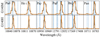 |
Fig. 1. Post-pixelized Gaussian profile fits (orange) to prominent emission-line groups (black) in the NIRSpec IFS spectra of the PN SMP LMC 58. The IFS mode G140 disperser is illustrated here as an example among the nine combinations analyzed in this letter. The top row corresponds to the G140M/F100LP configuration (i.e., medium resolution), and the bottom row to G140H/F100LP (i.e., high resolution). The principal line within each group is annotated in the corresponding panel. The individual line wavelengths fitted in each group are marked with dashed blue lines. All of these lines are fitted simultaneously to directly constrain the parameters in σinst′(λ) from Eq. (2). |
3.2. Measurement of the PN expansion velocity
To measure the expansion velocity of the PN from the X-shooter spectrum, we require a precise measurement of the spectral resolution of the X-shooter itself. We used the arc-lamp spectrum that was taken for wavelength calibration to obtain a wavelength-dependent estimate of X-shooter’s spectral resolution. We used the PYPEIT software program (Prochaska et al. 2020) to measure the FWHMs of the arc-lamp lines in 15 wavelength bins within the covered wavelength range of 550–1020 nm (Fig. 2). The uncertainty of the binned measurement was derived from the scatter in the individual-line measurements within each bin. The extent of the variation in the measured resolutions across the wavelength is qualitatively similar to that measured by Gonneau et al. (2020). We fit a quadratic function Rxsh(λ) to the measured points. We also simultaneously fit a post-pixelized Gaussian function to the Hα line, which is the most prominent H line within the covered wavelengths. Although a few He lines also fall within the covered wavelength range, they do not significantly add to the constraining power, due to their line strengths being smaller by 1.5 orders of magnitude or more. We parameterized the Hα line’s Gaussian profile with a standard deviation [σPN2 + c2/{2.355Rxsh(λHα)}2]−1/2, while allowing the peak position to vary to account for the PN’s relative motion. We constrained the PN’s expansion velocity to σPN = 6.90 ± 0.49 km s−1.
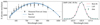 |
Fig. 2. Measurement of the PN’s expansion velocity. Left panel: Measurement of the X-shooter resolution (black points with error bars) from arc-lamp lines with the wavelength dependence modeled with a quadratic function (blue line, with the shaded region showing 1σ uncertainty). Right panel: The Hα line of the PN in the X-shooter spectra (emerald points). The error bars are too small to be seen here. The best-fit post-pixelized Gaussian profile is shown in red, while the width of the X-shooter LSF, as determined by the best fit in the left panel, is shown in blue for comparison. Both sets of illustrated datapoints are simultaneously fit to infer the PN’s expansion velocity σPN = 6.90 ± 0.49 km s−1. |
We illustrate the measured resolution curves for all the mode–disperser combinations in Fig. 3 and compare them to the corresponding pre-launch estimates provided by JDox. The resolutions in the IFS mode across the covered wavelengths are higher by ∼1–24% than the pre-launch estimates, whereas the resolutions in the FS mode are ∼11–53% higher.
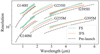 |
Fig. 3. Comparison of our measured resolution curves in the FS (emerald) and IFS (orange) modes with the pre-launch estimates from JDox (dashed gray lines). The shaded region around each resolution curve signifies the 1σ credible region. The in-flight resolutions are 11–53% higher than the pre-launch estimates in the FS mode, and 1–24% higher in the IFS mode (across the covered wavelengths). |
4. Conclusion
In this letter we measured NIRSpec’s spectral resolution in multiple configurations in the FS and IFS modes. Due to the similarity in slit dimensions, the FS mode resolution can be used as a reasonable proxy for the MOS mode. We provided a wavelength-dependent parameterization of the spectral resolution in terms of the instrumental dispersion σinst by fitting multiple H and He emission lines across the observed wavelength range in the PN SMP LMC 58. We incorporated a correction for the intrinsic width of the PN’s lines, which we measured using a higher-resolution X-shooter spectrum of the same PN. Our measured resolutions are directly applicable for point source spectra; however, caution is advised when using them for extended sources.
The measured resolutions increase with wavelength in all configurations, as expected from the pre-launch estimates provided by JDox. For the FS mode, our measured resolution values extend up to 20% higher than those found by Isobe et al. (2023), potentially due to our methodology allowing multiple lines to be fitted within a blended line group. Our measured resolution in the G140H/F100LP configuration is smaller than that found by Nidever et al. (2024), which may be a difference between single-exposure and stacked spectra. Therefore, caution is advised when applying our measured value for datasets with drastically different dithering procedures from CAL-1492.
The parametric wavelength-dependent functions we provide will enable accurate measurements of kinematics from the NIRSpec data, as performed by TDCOSMO Collaboration (2025) and Shajib et al. (2025), among others. Although we do not provide directly measured LSFs in the MOS mode, the FS mode values can be used as a substitute, following Isobe et al. (2023), as the slit width for the analyzed data in the FS mode is the same as that of the multi-shutter-array slitlets.
We did not utilize the MOS mode observations from the program CAL-1492, as the exposures were stepped at 25 mas steps across the full pitch of an MSA shutter. Thus, the LSF in the stacked data is expected to have broadened beyond that from a point source centered on the slit with only subpixel dithers applied. However, due to the similarity of the S200A1 slit dimension to the MSA shutters, the FS mode values are theoretically expected to be a reasonable proxy for MOS mode observations. Suitable MOS mode datasets in the future can be easily analyzed with the code suite and notebooks we provided.
v.300b5: https://linelist.pa.uky.edu/newpage/
Acknowledgments
We thank David Nidever for helpful comments as the referee, which improved this manuscript. We thank Hsiao-Wen Chen, Danial Rangavar Langeroodi, Mark Morris, and Stefan Noll for useful discussions. This work is based on observations made with the NASA/ESA/CSA James Webb Space Telescope. The data were obtained from the Mikulski Archive for Space Telescopes at the Space Telescope Science Institute, which is operated by the Association of Universities for Research in Astronomy, Inc., under NASA contract NAS 5-03127 for JWST. These observations are associated with programs #1125 and 1492. The specific observations analyzed can be accessed via https://dx.doi.org/10.17909/m3c0-3t58. AJS and TT acknowledge support from NASA through STScI grants JWST-GO-2974, HST-GO-16773, and JWST-GO-1794. This research made use of NUMPY (Oliphant 2015), SCIPY (Jones et al. 2001), ASTROPY (Astropy Collaboration 2013, 2018), JUPYTER (Kluyver et al. 2016), MATPLOTLIB (Hunter 2007), SEABORN (Waskom et al. 2014), and NAUTILUS (Lange 2023).
References
- Astropy Collaboration (Robitaille, T. P., et al.) 2013, A&A, 558, A33 [NASA ADS] [CrossRef] [EDP Sciences] [Google Scholar]
- Astropy Collaboration (Price-Whelan, A. M., et al.) 2018, AJ, 156, 123 [Google Scholar]
- Böker, T., Beck, T. L., Birkmann, S. M., et al. 2023, PASP, 135, 038001 [CrossRef] [Google Scholar]
- Bushouse, H., Eisenhamer, J., Dencheva, N., et al. 2023, https://doi.org/10.5281/zenodo.10022973 [Google Scholar]
- Cappellari, M. 2017, MNRAS, 466, 798 [Google Scholar]
- Cappellari, M. 2023, MNRAS, 526, 3273 [NASA ADS] [CrossRef] [Google Scholar]
- de Graaff, A., Rix, H.-W., Carniani, S., et al. 2024, A&A, 684, A87 [NASA ADS] [CrossRef] [EDP Sciences] [Google Scholar]
- D’Eugenio, F., Pérez-González, P. G., Maiolino, R., et al. 2024, Nat. Astron., 8, 1443 [CrossRef] [Google Scholar]
- Euclid Collaboration (Paterson, K., et al.) 2023, A&A, 674, A172 [NASA ADS] [CrossRef] [EDP Sciences] [Google Scholar]
- Gonneau, A., Lyubenova, M., Lançon, A., et al. 2020, A&A, 634, A133 [NASA ADS] [CrossRef] [EDP Sciences] [Google Scholar]
- Hunter, J. D. 2007, Comput. Sci. Eng., 9, 90 [NASA ADS] [CrossRef] [Google Scholar]
- Isobe, Y., Ouchi, M., Nakajima, K., et al. 2023, ApJ, 956, 139 [NASA ADS] [CrossRef] [Google Scholar]
- Jacob, R., Schönberner, D., & Steffen, M. 2013, A&A, 558, A78 [NASA ADS] [CrossRef] [EDP Sciences] [Google Scholar]
- Jones, E., Oliphant, T., Peterson, P., et al. 2001, SciPy: Open Source Scientific Tools for Python [Google Scholar]
- Jones, O. C., Álvarez-Márquez, J., Sloan, G. C., et al. 2023, MNRAS, 523, 2519 [Google Scholar]
- Kluyver, T., Ragan-Kelley, B., Pérez, F., et al. 2016, in Positioning and Power in Academic Publishing: Players, Agents and Agendas, eds. F. Loizides, & B. Schmidt (Amsterdam, Netherlands: IOS Press BV), 87 [Google Scholar]
- Knabel, S., Mozumdar, P., Shajib, A. J., et al. 2025, A&A, in press, https://doi.org/10.1051/0004-6361/202554229 [Google Scholar]
- Lange, J. U. 2023, MNRAS, 525, 3181 [NASA ADS] [CrossRef] [Google Scholar]
- Modigliani, A., Goldoni, P., Royer, F., et al. 2010, in Observatory Operations: Strategies, Processes, and Systems III, 7737, 773728 [Google Scholar]
- Newman, A. B., Gu, M., Belli, S., et al. 2025, arXiv e-prints [arXiv:2503.17478] [Google Scholar]
- Nidever, D. L., Gilbert, K., Tollerud, E., et al. 2024, in Early Disk-Galaxy Formation from JWST to the Milky Way, eds. F. Tabatabaei, B. Barbuy, & Y. S. Ting, IAU Symp., 377, 115 [Google Scholar]
- Oliphant, T. E. 2015, Guide to NumPy, 2nd edn. (USA: CreateSpace Independent Publishing Platform) [Google Scholar]
- Prochaska, J., Hennawi, J., Westfall, K., et al. 2020, JOSS, 5, 2308 [NASA ADS] [CrossRef] [Google Scholar]
- Reid, W. A., & Parker, Q. A. 2006, MNRAS, 373, 521 [NASA ADS] [CrossRef] [Google Scholar]
- Shajib, A. J., Treu, T., Suyu, S. H., et al. 2025, A&A, submitted [arXiv:2506.21665] [Google Scholar]
- TDCOSMO Collaboration 2025, A&A, submitted [arXiv:2506.03023] [Google Scholar]
- van Hoof, P. A. M. 2018, Galaxies, 6, 63 [NASA ADS] [CrossRef] [Google Scholar]
- Vernet, J., Dekker, H., D’Odorico, S., et al. 2011, A&A, 536, A105 [NASA ADS] [CrossRef] [EDP Sciences] [Google Scholar]
- Waskom, M., Botvinnik, O., Hobson, P., et al. 2014, https://doi.org/10.5281/zenodo.12710 [Google Scholar]
- Xu, Y., Ouchi, M., Yajima, H., et al. 2024, ApJ, 976, 142 [Google Scholar]
Appendix A: Fitted line lists
In this appendix we provide the list of fitted lines within the chosen wavelength ranges in Tables A.1, A.2, and A.3 for the G140, G235, and G395 dispersers, respectively. We first obtained a comprehensive list of nebular H and He lines from the Atomic Line List database6 (van Hoof 2018). We then aggregated the He lines that are close to each other within one-eighth of a pixel size in the corresponding high-resolution spectrum into a single line with an average wavelength weighted by the transition probability (i.e., the Einstein coefficient gkAki). We adopted one-eighth of the pixel size here, as this is one-half of the target threshold for wavelength calibration error (Böker et al. 2023). Thus, lines that are separated more closely can be sufficiently considered indistinguishable in the spectrum. Not all the line groups were fitted in some modes, as those line groups fall fully or partially outside of the covered wavelength range in the particular modes. The tables in this appendix specify the modes for which each line group was fitted.
Line list in the fitted wavelength ranges for the G140 disperser.
Line list in the fitted wavelength ranges for the G235 disperser.
Line list in the fitted wavelength ranges for the G395 disperser.
All Tables
All Figures
|
Fig. 1. Post-pixelized Gaussian profile fits (orange) to prominent emission-line groups (black) in the NIRSpec IFS spectra of the PN SMP LMC 58. The IFS mode G140 disperser is illustrated here as an example among the nine combinations analyzed in this letter. The top row corresponds to the G140M/F100LP configuration (i.e., medium resolution), and the bottom row to G140H/F100LP (i.e., high resolution). The principal line within each group is annotated in the corresponding panel. The individual line wavelengths fitted in each group are marked with dashed blue lines. All of these lines are fitted simultaneously to directly constrain the parameters in σinst′(λ) from Eq. (2). |
| In the text | |
|
Fig. 2. Measurement of the PN’s expansion velocity. Left panel: Measurement of the X-shooter resolution (black points with error bars) from arc-lamp lines with the wavelength dependence modeled with a quadratic function (blue line, with the shaded region showing 1σ uncertainty). Right panel: The Hα line of the PN in the X-shooter spectra (emerald points). The error bars are too small to be seen here. The best-fit post-pixelized Gaussian profile is shown in red, while the width of the X-shooter LSF, as determined by the best fit in the left panel, is shown in blue for comparison. Both sets of illustrated datapoints are simultaneously fit to infer the PN’s expansion velocity σPN = 6.90 ± 0.49 km s−1. |
| In the text | |
|
Fig. 3. Comparison of our measured resolution curves in the FS (emerald) and IFS (orange) modes with the pre-launch estimates from JDox (dashed gray lines). The shaded region around each resolution curve signifies the 1σ credible region. The in-flight resolutions are 11–53% higher than the pre-launch estimates in the FS mode, and 1–24% higher in the IFS mode (across the covered wavelengths). |
| In the text | |
Current usage metrics show cumulative count of Article Views (full-text article views including HTML views, PDF and ePub downloads, according to the available data) and Abstracts Views on Vision4Press platform.
Data correspond to usage on the plateform after 2015. The current usage metrics is available 48-96 hours after online publication and is updated daily on week days.
Initial download of the metrics may take a while.