| Issue |
A&A
Volume 702, October 2025
|
|
|---|---|---|
| Article Number | A208 | |
| Number of page(s) | 12 | |
| Section | Galactic structure, stellar clusters and populations | |
| DOI | https://doi.org/10.1051/0004-6361/202556434 | |
| Published online | 17 October 2025 | |
Black hole mass function shift in proto-stellar clusters driven by gas accretion
1
Dipartimento di Fisica “G. Occhialini”, Universitá degli Studi di Milano-Bicocca,
Piazza della Scienza 3,
20126
Milano,
Italy
2
Istituto Nazionale di Fisica Nucleare (INFN), Sezione di Milano-Bicocca,
Piazza della Scienza 3,
20126
Milano,
Italy
★ Corresponding author: This email address is being protected from spambots. You need JavaScript enabled to view it.
Received:
16
July
2025
Accepted:
10
September
2025
Abstract
The James Webb Space Telescope (JWST) has observed compact, massive proto-stellar clusters of low metallicity in the Cosmic Gems arc galaxy at high redshift, which represent likely precursors to globular clusters. We model the mass growth of stellar black holes (BHs) during the first few million years of the life of a massive, compact, gaseous stellar cluster before stellar feedback expels the primordial gas. At high redshift, in a lower-metallicity environment stellar winds get weaker, allowing for larger gas-depletion timescales in the cluster despite energetic pair-instability supernova (PISN) feedback for sufficiently compact clusters. Mass segregation drives the massive stellar progenitors of BHs in the center of the cluster, where gas is densest. We estimate the conditions for which the initial black hole mass function (BHMF), with a PISN-induced cutoff of <55 M⊙, gets shifted to values within the upper BH mass gap, ~60–130 M⊙, or higher, as observed by the LIGO-Virgo-KAGRA gravitational wave (GW) experiments. We find that the BHs are shifted by the end of gas depletion to values within and above the mass gap, well within the range of BH components of the recent GW-signal GW231123, depending on the total mass, star formation efficiency, metallicity, and compactness. The individual BH mass increase approximately follows a surprisingly steep power law with respect to the initial BH mass with an exponent in the range of ≈4–6. This occurs in gaseous proto-stellar clusters that are sufficiently massive and compact, with typical values for the total mass of ~106 M⊙ and size of ~1 pc. Our analysis suggests that proto-stellar clusters at high redshift such as Cosmic Gems arc clusters have generated through early gas accretion, BHs as heavy as ~102−103 M⊙.
Key words: gravitational waves / stars: black holes / stars: massive / supernovae: general / galaxies: star clusters: general
© The Authors 2025
 Open Access article, published by EDP Sciences, under the terms of the Creative Commons Attribution License (https://creativecommons.org/licenses/by/4.0), which permits unrestricted use, distribution, and reproduction in any medium, provided the original work is properly cited.
This article is published in open access under the Subscribe to Open model. This email address is being protected from spambots. You need JavaScript enabled to view it. to support open access publication.
1 Introduction
Recent JWST observations reveal the existence of proto-stellar clusters in the Cosmic Gems arc galaxy that are at high redshift, z = 10.2, younger than 50 Myr, of low metallicity, and remarkably compact, with typical masses of ~106 M⊙ and half-light radii of ~1pc (Adamo et al. 2024). Such proto-stellar clusters are plausibly the progenitors of globular clusters (GCs) (Kruijssen 2015; Renzini 2017; Zick et al. 2018; Elmegreen 2018; Vanzella et al. 2020), while they may be also relevant to the formation of nuclear star clusters (NSCs) (Guillard et al. 2016; Neumayer et al. 2020). These JWST-observed proto-stellar clusters share similar characteristics with super star clusters (SSCs), considered to be young GCs, observed in the past by Hubble Space Telescope (HST) at low-z, though they are somewhat less, but comparably, compact, have subsolar metallicities, and are observed at an age (<5 Myr) when they still have residual gas content (Ho & Filippenko 1996; De Marchi et al. 1997).
Therefore, the existence of proto-stellar clusters, i.e., compact, massive stellar clusters with low or subsolar metallicity that retain residual gas for several million years is established obser-vationally. It is possible that BHs in these clusters have enough time to accrete gas before stellar winds and SN explosions expel the primordial gas (Roupas & Kazanas 2019b). Lower metallicity implies weaker stellar winds. Higher compactness allows more pristine gas to survive the SN explosions. The progenitors of BHs are the most massive stars, and therefore accumulate in the core of the cluster, where gas density is higher, due to mass segregation (Spitzer 1987; Leigh et al. 2014).
Identifying formation mechanisms of BHs with masses of 60 M⊙ ≲ mBH ≲ 103 M⊙ is a topical, timely, flourishing research subject in astrophysics and especially GW astronomy (Gerosa & Berti 2017; Roupas & Kazanas 2019b; Baibhav et al. 2020; Renzo et al. 2020; Kimball et al. 2020; Safarzadeh & Haiman 2020; Mapelli et al. 2021; Rizzuto et al. 2022; Arca Sedda et al. 2023; Torniamenti et al. 2024; Fujii et al. 2024; Purohit et al. 2024; Baumgarte & Shapiro 2025; Lee et al. 2025; Bartos & Haiman 2025). Gravitational wave (GW) experiments, the LIGO Scientific Collaboration, the Virgo Collaboration, and the KAGRA Collaboration (Abbott et al. 2023) have revealed a significant population of BHs within the theorized upper BH mass gap of 60 M⊙ ≲ mBH ≲ 130 M⊙, induced by the physics of a pair-instability supernova (PISN) (Belczynski et al. 2016; Spera & Mapelli 2017; Woosley & Heger 2021). During the completion of this work, LIGO-Virgo-KAGRA reported the GW signal GW231123 (The LIGO Scientific Collaboration et al. 2025) involving two heavy BHs with masses of  and
and  . The typical formation channel for such masses is the repeated mergers channel (Miller & Hamilton 2002; O’Leary et al. 2006; Gerosa & Berti 2017). Here, we suggest another, not mutually exclusive, formation channel.
A second reason for the significance of this BH mass range is the potential to explain the observed abundance and masses of supermassive BHs (SMBHs) at high redshifts (Larson et al. 2023; Bogdán et al. 2024; Regan & Volonteri 2024). This issue is also closely related to the Laser Interferometer Space Antenna (LISA) astrophysics research (Amaro-Seoane et al. 2023).
The major goals of this work are firstly to identify the physical conditions under which the stellar BHs assumed to be generated with a mass cutoff, mBH < 55 M⊙, inside proto-stellar clusters accrete sufficient amount of gas to populate the upper BH mass gap before the gas gets depleted due to stellar formation feedback, and secondly to quantify this shift of the BH mass function of a BH population in a proto-stellar cluster. We find that under certain conditions it is possible that a BH grows as massive as ~103 M⊙. We therefore provide not only a new physically motivated formation channel of mass-gap-BHs, but also a pathway from stellar-mass to intermediate-mass-BH (IMBH) seeds.
In the next section we calculate gas depletion timescales. In Section 3 we present our physical model. In Section 4 we discuss our results. We conclude in the final section.
2 Gas depletion timescale
Gas expulsion in gaseous stellar clusters is driven by the energy and momentum from stellar winds and supernovae injected to the ambient gas. Additionally, the stellar lifetimes determine not only the moment of time where SNe occur, and therefore the time distribution of their energy injection, but also the birth time of BHs from their stellar progenitors. We analytically modeled the stellar winds and SN energy injection, and the stellar lifetimes, with respect to stellar mass and metallicity, according to observational and numerical data. We estimated the depletion timescale as the moment of time when the accumulated injected energy equals the initial binding energy of the gas, counting from the time when all stars are born.
2.1 Winds
The stellar winds of solar-type intermediate-mass stars of m < 8 M⊙ contribute negligible energies within the depletion timescales of ~0.1–10 Myr (e.g., Leitherer et al. 1999) with respect to the more massive stars of m > 8 M⊙. Therefore, we considered only the latter cases.
We modeled the injected mechanical luminosity of stellar winds using a piecewise power fit (Kudritzki 2002; Puls et al. 2008),
 (1)
(1)
where Lref is the reference mechanical luminosity at solar metallicity for the reference mass scale, mref, and Lref, α, and mref take different values in three distinct mass segments,
 (2)
(2)
We used these values based on existing data (Vink et al. 2001; Repolust et al. 2004; Hamann et al. 2006; Crowther 2007; Bestenlehner et al. 2011; Vink 2017; Renzo et al. 2017; Sander & Vink 2020) and to ensure continuity in the break-points allowing for efficient numerical operations. In more detail, we assumed that Lref = 7 ∙ 1036 erg/s for mref = 20 M⊙ (Repolust et al. 2004), Lref = 1038 erg/s for mref = 60 M⊙ (Hamann et al. 2006; Crowther 2007; Vink 2017; Sander & Vink 2020), Lref = 2.5 ∙ 1038 erg/s for mref = 120 M⊙ (Bestenlehner et al. 2011), at solar metallicity. We calibrated those and the power exponents to ensure continuity at the breakpoints, while satisfying the general slope trend – OB stars follow a steeper profile than WR stars (Vink et al. 2001; Repolust et al. 2004); for the very massive stars (>120 M⊙) the curve flattens Sander & Vink (2020) – and respecting theoretical and observational limits (Vink et al. 2001 ; Renzo et al. 2017). Finally, we adopted a single, population-averaged, metallicity exponent factor, fZ = 0.8, for all stars of m ≥ 8 M⊙ (Vink et al. 2001; Crowther 2007; Renzo et al. 2017). This average exponent is sufficient for our main purpose, which is to get an approximate estimate of the gas depletion timescale, capturing the essential property that massive stars’ wind energy depends strongly on metallicity.
The wind energy is subject to losses and redistribution inside the cluster (Krause et al. 2013; Dale et al. 2014). We adopted a wind feedback efficiency of 0.1 (Silich et al. 2003; Krause et al. 2013; Dale et al. 2014; Geen et al. 2015). This includes not only energy loss (radiative cooling, mixing, leakage, incomplete coupling, and so on), but also the fraction of energy that is distributed inefficiently (translational energy converted to rotational –turbulence – geometry, and so on), so that only the energy that is actually used for gas expulsion is assumed to be counted.
2.2 SNe
For core-collapse SNs (CCSNe), we set a lower mZAMS at 8 M⊙ and a maximum possible mZAMS that increases with decreasing metallicity, particularly at 30 M⊙, 35 M⊙, and 40 M⊙ for solar, subsolar (~0.1 Z⊙), and low (~0.01 Z⊙) metallicities, respectively (e.g., Heger & Woosley 2002; Heger et al. 2003; Nomoto et al. 2006; Sukhbold et al. 2016). The tabulated data of Woosley & Weaver (1995) can be approximated, sufficiently for our purposes, with a simple second-order polynomial fit for solar, subsolar, and low metallicities, respectively, as
 (3)
(3)
which give energies of ∼(4–4.5) ∙ 1050 erg for a 20 M⊙ star depending on the metallicity.
Regarding pulsational pair-instability SNe (PPISNe) and pair-instability SNe (PISNe), we find that tabulated and plotted data of PPISNe (Woosley 2017) and PISNe (Heger & Woosley 2002; Kasen et al. 2011) are effectively modeled by simple linear fits. For PPISN we adjusted E = 1050 erg for mZAMS = 80 and E = 1051 erg for mZAMS = 125 (Woosley 2017),
 (4)
(4)
For PISN we adjusted E = 5 ∙ 1051 erg for mZAMS = 140 M⊙ and E = 5 ∙ 1052 erg for mZAMS = 230 M⊙ (Heger & Woosley 2002; Kasen et al. 2011),
 (5)
(5)
We assumed that PISNe can occur only at low metallicity, while PPISN occur at both subsolar and low metallicity.
Only a fraction of the total energy generated by a SN explosion contributes efficiently to the depletion of the ambient gas (Krause et al. 2013; Pittard 2019; Watkins et al. 2023). We adopted a SN feedback efficiency equal to 0.1 in agreement with recent observations (Watkins et al. 2023).
We assumed a Kroupa piecewise initial mass function (IMF) for the stars (Kroupa 2002) with slopes of 0.3, 1.3, and 2.3 for the low-mass (0.01 ≤ m < 0.08), intermediate-mass (0.08 ≤ m < 0.5), and high-mass (0.5 ≤ m < mmax) regimes, respectively. We assumed mmax = 135 M⊙ for the solar and subsolar metallicity cases and mmax = 230 M⊙ for the low-metallicity case. We calculated the stellar lifetimes, extrapolating the tabulated data of Ekström et al. (2012) for solar metallicity, the data of Georgy et al. (2013) for subsolar metallicity (Z = 0.002), and the data of Groh et al. (2019) for low metallicity (Z = 0.0004).
2.3 Depletion timescale estimation
The binding energy, U ∝ M2/R ~ C ∙ M, grows linearly with the total mass of the cluster, M, for a fixed initial compactness, C, defined as
 (6)
(6)
The feedback energy, on the other hand, grows as Efeed ∝ M regardless of the compactness. Therefore, the effectiveness of gas depletion (depletion timescale) depends solely on the compactness, C, and of course the star formation efficiency, ε, not on the mass of the cluster. This basic energy scaling also suggests that for all clusters of any mass there should exist some upper compactness, above which gas expulsion is ineffective (see also Krause et al. 2016).
The star formation efficiency is the other sensitive factor affecting the depletion timescale. Observational evidence at high redshift suggests a range of ε ≈ 0.05–0.3 (Inayoshi et al. 2022). At z ≈ 1 observations suggest a typical value in giant molecular clouds of ε ≈ 0.1 (Dessauges-Zavadsky et al. 2019, 2023). We consider in our analysis the range ε = 0.05–0.35.
In Figure 1, we depict the depletion timescale with respect to compactness for several ε values and metallicities. We assume that in subsolar metallicity, Figure 1b, there occur PPISNe, but not an energetic PISN. At low metallicity, Figure 1c, we consider that PISN do take place.
Notice that for solar metallicity, although we consider the case that no PPISN and PISN operate, the timescale is shorter with respect to similar ε and C than in the subsolar and low-metallicity cases, because stellar winds are more severe. For the subsolar and low-metallicity cases, compactness values of C ≳ 10 have depletion timescales of τ ≳ 3 Myr, high enough for BHs from sufficiently massive stars be generated early enough to accrete gas before it gets depleted, as we verify in detail below. Particularly significant is the plateau in the low-metallicity case at τ ≃ 3 Myr for 2 ≲ C ≲ 30. It signifies the ignition of PISN. These energetic SNs do not allow for the depletion timescale to increase even if compactness of the cluster is increased and/or stellar formation is decreased. This overlaping of τ for several ε and C values allows for larger ε values to be as, or more, efficient regarding black hole mass function (BHMF) shift as lower ε values, because higher ε correspond to less diluted gas density profiles. We calculate this in detail below.
3 Physical model
For a given compactness, total cluster mass, star formation efficiency, and metallicity, we calculated the gas depletion timescale, τ, generated a BH population with each BH generated at a different time depending on the ZAMS progenitor mass, and evolved these BHs in background gas and density Plummer profiles, taking into account the expansion of the cluster due to the mass loss. We integrated the BHs equations of motion and accretion rate using a standard drift-kick scheme, with the deterministic forces – gravity and dynamical friction – evolved using an adaptive Runge-Kutta method and stochastic velocity increments, due to stellar perturbations and gas turbulence, applied at adaptive timesteps. We applied an additional recoil kick to the BH remnants of CCSN. This kick drives the majority of these types of BHs out of the cluster.
We assumed that BH close encounters are implicitly considered in the stochastic stellar kicks calculation, i.e., we did not consider the BHs’ mutual gravity separately. This allowed us to investigate a vast range of physical parameters, saving numerical time. The self-gravity of the BH population would be important if one calculated the formation of binary BHs and for significantly larger timescales, which we do not do here. In any case, the BH population contributes negligible gravity with respect to the stellar population and in addition each BH enters the simulation in its own moment of time. In numbers, for example, a 106 M⊙ cluster generates ~1000 BHs, out of which ~70% escape at birth. The remaining 300 BHs not only have negligible self-gravity with respect to the combined gas and stellar background but also each one enters the simulation in its own moment of time (depending on progenitor’s ZAMS mass) over a range of ~10 Myr when our simulations approximately terminate. Also, out of the 300 BHs, a fraction, ~50 BHs, do undergo a significant mass increase.
Since the stellar feedback processes that expel the gas generate energy proportional to the cluster mass, it is natural to consider an exponential law, Ṁgas = –Mgass/τ, of gas depletion (Baumgardt & Kroupa 2007). We additionally assumed that the gas loss due to accretion onto BHs is already implicitly considered in this exponential law of gas depletion. This is justified as long as the total accreted mass is negligible with respect to the gas reservoir and certainly less than the remaining gas when we terminate the simulation. In practice, for all the simulations we present here the BHs do not accrete more than ≲0.5% of the initial gas reservoir, while we terminated the simulation when exactly 99% of the initial gas had depleted.
We assumed, furthermore, that the cluster expands according to the well-known adiabatic invariant (Hills 1980)
 (7)
(7)
This assumes that the system remains nearly in virial equilibrium during gas depletion. This is sufficient for our purposes and is a good approximation of the τ ≳ 3 Myr cases that we consider here, improving the efficiency of our numerical code, while taking into consideration cluster dilution due to mass loss.
The gas profile should naturally be more extended than the stellar component (e.g., Johnson et al. 2015; Kruijssen et al. 2019). We assumed that
 (8)
(8)
The b = 1 would correspond to both components being equally compact. We calibrated b such that rh,gas = 5 rh,star for ε = 0.1 (Parmentier & Pfalzner 2013), which gives b = 0.73 and corresponds to a gaseous component that is less dense than the stellar component (ρh,gas = 0.07ρh,stars) and significantly more extended.
The gas temperature evolves as the cluster loses mass. We modeled the temperature evolution with a typical logarithmic scaling (Dopita & Sutherland 2003),
 (9)
(9)
where T0(t) is the central temperature with respect to time, and we set Tini = 1.2 × 10⁴ K the initial central temperature, Tfin = 4 × 10³ K the final central temperature when gas is 99% depleted. We further denote M(t) = M★ + Mgas(t) the total cluster mass, and M0 the initial total cluster mass. The thermal central velocity dispersion is related to temperature through σ0,T(t)2 = kBT0(t)/meff, where meff = 0.6 mp is the effective particle mass for the ionized gas, and we assume στ(r, t) follows the Plummer profile with σΤ(r = 0, t) = σ0,T(t). The local sound speed is then directly given by  , where γ = 5/3 is the adiabatic index.
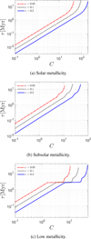 |
Fig. 1 Our estimated depletion timescale, τ, with respect to the compactness, C, of a gaseous stellar cluster of any total mass. We considered three possible star formation efficiencies, ε. Each sub-figure (a), (b), (c) corresponds, respectively, to solar, subsolar (~0.1 Z⊙), and low (~0.01 Z⊙) metallicity. We assume that at subsolar metallicity PPISN operates, and that in the low-metallicity case both PPISN and PISN do. |
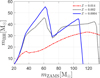 |
Fig. 2 BH-remnant mass with respect to the ZAMS progenitor’s mass, reproduced from Spera & Mapelli (2017), used here in determining the BH entry time in our simulation. |
3.1 BH generation
We generated the BH population stochastically, assigning as the BH IMF a Salpeter mass function (Perna et al. 2019) with a power exponent equal to 2.37. We want to evaluate the shift of the BH IMF to higher mass values, which is why we want to have a definite power exponent for the BH IMF, which we can directly compare to the shifted BHMF after the gas gets depleted (at our fixed 99% threshold). For the BH IMF, we assumed a minimum BH mass of 5 M⊙ and a maximum BH mass that depends on the metallicity; that is, 55 M⊙ for low metallicity, 45 M⊙ for sub-solar metallicity, and 33 M⊙ for solar metallicity. These values were extracted from the zero-age main sequence (ZAMS) progenitor versus BH mass Figure 2 of Spera & Mapelli (2017), which includes PPISN and PISN. For completeness, we reproduce this data here, in our Figure 2. We assigned a ZAMS mass to each BH based on Figure 2 and if several possible ZAMSs existed we also assigned a probability assuming a stellar Kroupa IMF as is described in Section 2.2. Then, each BH entered the simulation at its own moment of time equal to the lifetime of the ZAMS progenitor assigned to it.
We further categorized the BHs depending on their formation type. If the ZAMS mass lay in the CCSN range we assigned the CCSN-BH type, if it lay in the range between the maximum CCSN and minimum PPISN thresholds we assigned it the direct-collapse-BH type, and if it lay in the PPISN range we assigned the type PPISN-BH. However, there are some additional considerations stemming from the Figure 2. We can see that for subsolar and low metallicity there are two peaks. The first peak signifies the minimum possible mass loss during direct collapse. Between the peaks stars enter the PPISN regime where multiple pulsations eject significant envelope mass. At the second peak, stars eject the minimum possible mass through pulsations to drop below the pair-instability threshold, still allowing the remaining core to collapse into a BH. Beyond some ZAMS mass value complete PISN occurs, totally disrupting the star with no remnant. Therefore, we further subcategorized the direct-collapse-BHs born from ZAMS on the left part of the first peaks as direct-collapse-BHs from low ZAMS and those from the valley between the peaks as direct-collapse-BHs from high ZAMS. Likewise, we have PPISN-BHs from low ZAMS for those generated from the valley between the peaks and PPISN-BHs from high ZAMS for those generated from the right part of the second peak.
We assumed that the massive stellar progenitors had undergone mass segregation and reached Brownian equilibrium within the stellar profile (Roupas 2021). Consequently, we sampled the initial BH position from the Roupas (2021) profile,  . We sampled the initial BH velocities from a Maxwell distribution using Jeans theorem for this density profile.
Black holes formed by direct collapse, in the absence of energetic mass loss, are not expected to receive significant kick velocities (Shenar et al. 2022). This is also the case for PPISN-formed BHs. The PPISN pulses expel most of the envelope prior to core collapse, so that the final core implosion proceeds as an almost spherically symmetric direct-collapse event, with the resulting BH receiving at most a few kilometers per second kicks (Rahman et al. 2022). We therefore assumed that direct-collapse-BHs and PPISN-BHs attain the kicks’ magnitude, at most comparable to the 1D rms velocity of the stellar progenitor, and therefore that the kicks’ contribution to the initial BH velocity is implicitly considered in our random initial BH-velocity generator. On the other hand, the CCSN-BHs are expected to receive significant natal kicks due to asymmetries in the explosion (e.g., Mandel 2016). The CCSN remnants are reasonably expected to attain kick velocities that follow a Maxwellian (Hobbs et al. 2005). For CCSN-BHs we adopted a prescription similar to Giacobbo & Mapelli (2020) for the 1D rms velocity of the natal kicks, σΝΚ, of the Maxwellian distribution; that is,  . We calibrated it to account for the possibility of kicks as high as 100 km/s (O’Shaughnessy et al. 2017; Atri et al. 2019), assuming σΝK = 50 km/s ∙ (mBH/10)–1 for CCSN-BHs.
3.2 Gas accretion
In the dense, hot, turbulent gaseous environment that we considered, and given the BH motion at speeds comparable to but not significantly larger than the speed of sound, cs, it is justified to consider an isotropic hot-type accretion, whose typical representative is Bondi-Hoyle accretion (Merritt 2013). The spherically symmetric accretion rate, for a cross section of  , is (Frank et al. 1985)
 (10)
(10)
where the BH relative velocity is
 (11)
(11)
The proper accretion radius inside a gaseous stellar cluster depends on the relative amount of gas and on the radial position of the accretor (Bonnell et al. 2001). When gas is less dominant, the appropriate accretion radius is the Bondi-Hoyle radius, RB:
 (12)
(12)
However, the accretion rate is determined by a tidal-lobe accretion radius, when the gas dominates the cluster potential (Paczynski 1971),
 (13)
(13)
where M(r < ri) is the total mass of the cluster within the radial position, ri, of the ith BH. We chose the accretion radius to be the smaller of the two at any instant in time (Bonnell et al. 2001),
 (14)
(14)
adopting the most conservative assumption.
Inayoshi et al. (2016) have shown that for 1 < ṁfeed/ṁEdd,0 < 100 the mean accretion rate cannot exceed 〈ṁacc〉 ≲ 10ṁEdd,0. The quantity ṁEdd,0 = 4πGmBHmp/η0σTc is the reference Eddington rate value for the radiative efficiency η0 = 0.057. We therefore adopted a maximum threshold,
 (15)
(15)
This is a conservative assumption, especially at low metallicity and for thick disks. Inayoshi et al. (2016) report that though the mean accretion rate cannot exceed a few times the ṁEdd,0 (when ṁfeed < 100ṁEdd,0), there occur episodic bursts of accretion rate comparable to ṁfeed. In this regime the accretion rate is not strictly steady. We adopted a constant cap as a simple, conservative assumption. In practice, in the physical conditions we consider here, the ṁfeed we find is less than ≲10 M⊙/Myr for a 50 M⊙ BH, close to the Eddington accretion rate for a thick disk radiative efficiency, η ~ 0.01, which is about 5ṁEdd,0, i.e., below our applied threshold. The ṁfeed tends to attain values above our threshold when BHs approach masses of ~ 103 M⊙ in the physical conditions we consider here.
A concern might be that CCSN and PPISN events form dilute bubbles that expand rapidly around the progenitor star, and therefore whether the accretion rates we consider are appropriate for CCSN-BHs and PPISN-BHs. In our physical conditions, however, a BH formed from a CCSN or PPISN has sufficient time to escape the bubble, while the bubble itself has sufficient time to refill with gas. Specifically, the bubble’s maximum radius is given by the stalling formula  (McCray & Kafatos 1987), which is reached at time tstall = 0.4Rstall/cs (Sedov 1946; Taylor 1950), assuming that the shock stalls when υshock ≈ cs. The BH requires time tcross ~ Rstall/υBH to cross the bubble. The bubble refills on a timescale of trefill ~ Rstall/cs. For ESN ~ 1051–1052 erg, all of these timescales are on the order of 1–10 kyr. This is short compared to the timescale on which the BHMF-shift operates (~10 Myr). Even heavy BHs that are of low mobility have the opportunity to accrete gas because at these high temperatures the bubble refills rapidly relative to the accretion process timescale. Nevertheless, local conditions may stochastically suppress accretion for CCSN-BHs and PPISN-BHs. Therefore, our results are expected to be less accurate for CCSN-BHs and PPISN-BHs than for direct-collapse-BHs, which form without disrupting the gas in their immediate vicinity.
3.3 Dynamical friction
The deterministic forces applied to the BHs are the gravitational force from the stellar and gaseous background and the dynamical friction due to both components. We used the standard Chan-drasekhar dynamical friction formula to model the deceleration of BHs due to gravitational interactions with surrounding stars:
 (16)
(16)
where  , with σ★ the local stellar velocity dispersion. We denoted as υ the velocity of the BH, and the Coulomb logarithm is ln Λ = ln(bmax/bmin), with bmax = rcs and
  , where rcs is the stellar Plummer radius.
In a gaseous medium, the dynamical friction formula needs modification to account for the hydrodynamic nature of the interaction (Ostriker 1999)
 (17)
(17)
where cs is the sound speed in the gas and ℱ is a function that accounts for the Mach number, ℳ = υ/cs, dependence
 (18)
(18)
with ℱ → ln Λ in the singular limit ℳ → 1.
We added to this the deceleration due to the mass increase (Tanaka & Haiman 2009; Lee & Stahler 2011, 2014)
 (19)
(19)
which may be understood simply as manifesting angularmomentum preservation (Roupas & Kazanas 2019a).
3.4 Stellar stochastic kicks
The granularity of the stellar component induces local perturbations in the background mean gravitational field. We modeled these stochastic velocity perturbations on BHs through stellar encounters as a white noise process (e.g., Roupas 2021) derived from the fluctuation-dissipation theorem
 (20)
(20)
where ξ is a 3D Gaussian random vector with zero mean and unit variance and Δt is the timestep. We describe below our adaptive timestep formulation. The diffusion coefficient is
 (21)
(21)
The stellar dynamical friction coefficient, η★, follows from Chandrasekhar formula (16). The diffusion coefficient scales inversely with BH mass, ensuring that more massive BHs experience proportionally weaker stochastic velocity kicks.
3.5 Turbulent gas stochastic kicks
Gas turbulence is modeled as an Ornstein–Uhlenbeck (OU) process acting on the BH through a time-correlated turbulent acceleration field. OU is a well-defined stochastic process with a finite autocorrelation timescale and can be used to excite turbulent motions in simulations (Eswaran & Pope 1988; Schmidt et al. 2006; Federrath et al. 2010). It is generated by the OU stochastic differential equation,
 (22)
(22)
where dW is a 3D Wiener process, representing independent Gaussian white noise with zero mean and variance dt in each spatial component. We set the acceleration variance as
 (23)
(23)
and the correlation time depends on the turbulence Mach number, τOU = rcg/ℳcs if ℳ > 1 or τOU = rcg/cs otherwise.
The OU equation originates from the Langevin description of a particle subject to both linear damping and stochastic forcing. This formulation naturally produces time-correlated fluctuations with the autocorrelation function  , capturing the finite coherence time of turbulent eddies in the gaseous medium.
The OU-SDE (22) can be integrated directly to get the turbulent acceleration
 (24)
(24)
where ξ is a 3D Gaussian random vector with zero mean and unit variance. We can now integrate the OU acceleration (24) to get the corresponding velocity kick over timestep Δt,
 (25)
(25)
where ξ′ is an independent Gaussian random vector.
3.6 Adaptive timestep of stochastic kicks
We adaptively determined the integration timestep of both stellar and gas stochastic kicks for each BH based on the minimum of relevant physical timescales locally to ensure numerical stability and accuracy,
 (26)
(26)
where fdt is a safety factor with our default value of fdt = 0.5. We denote the dynamical timescale,  , the crossing timescale, τcross = rcs/υ, the dynamical friction timescale, τdf = 1/(η★ + ηgas), and the correlation time of the OU process, τOU.
The timestep is further constrained by prescribed bounds, Δtmin ≤ Δt ≤ Δtmax, with default values of Δtmin = 10–5 Myr, Δtmax = 0.1 Myr. In practice, these bounds are always satisfied. This approach is intended to ensure that the integration resolves the fastest relevant physical process while maintaining computational efficiency. We directly integrated the deterministic part – gravity and dynamical friction – between the stochastic timesteps using an adaptive Runge-Kutta method.
4 Results
We implemented three different studies. Firstly, we performed ten runs of a proto-stellar cluster with an initial total mass of 106 M⊙ for three combinations of ε, rh values for subsolar and low metallicity. These should represent the formation stage of typical GCs with a final stellar mass of ~105 M⊙. The results are summarized in Figures 3, 4 and Table 1. In the second study we provide a general picture of the effectiveness of our proto-BHMF-shift mechanism over a vast range of parameters. We ran multitude additional simulations to inspect the whole ε, rh space regarding the possibility of a proto-BHMF-shift for vastly different cluster initial total mass values of 105–7 M⊙, and for solar, subsolar, and low metallicities. These results are summarized in Figure 5. In the third study, we model a typical proto-stellar cluster of the recent JWST observations in the Cosmic Gems arc galaxy. These results are displayed in Figures 6 and 7. Finally we discuss the case of GW231123.
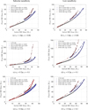 |
Fig. 3 Shifted BH masses, after stellar feedback expels 99% of the gas, with respect to the initial BH masses for a gaseous stellar cluster with total initial mass M = 106 M⊙ containing ~1000 BHs, for several star formation efficiency and half-mass radius, i.e., compactness, values of the cluster. Each subfigure was generated by a set of ten simulations. The left column corresponds to subsolar metallicity (~0.1 Z⊙), the right column to low metallicity (~0.01 Z⊙). The solar metallicity case, not shown here, requires about double or higher compactness to have the same effect as the subsolar case. |
4.1 M = 106 M⊙ proto-stellar clusters
In Figure 3, we depict scatter diagrams of the shifted BH masses with respect to the initial BH masses for the sets of values {rh, ε} = {0.1 pc, 0.06}, {0.07 pc, 0.1} and {0.5 pc, 0.2} at sub-solar and low metallicity for a cluster with an initial total mass of M = 106 M⊙. We varied ε with rh because the BHMF-shift requires lower ε as C is decreased (rh is increased) to be effective, while it is also physically motivated: the star formation efficiency increases for more compact clusters (lower rh), where the gas is more condensed. These cluster mass and half-mass radius values correspond to compactness values of C = 10, 14.3, 20. The values {M, rh} = {106 M⊙,0.07 pc} correspond to Figures 4c and 4d, where it is evident that, for ε = 0.1, in the low-Z case the whole upper BH mass gap is filled and spanned up to 150 M⊙. In the subsolar case, the BH masses reach up to ~450 M⊙. These masses of >150 M⊙ manifest as a tail in the shifted BHMF in Figure 4c. This is not special for the subsolar case, but can occur at any metallicity if the cluster is compact enough and/or the stellar formation efficiency is low enough, as we explain in detail below.
We observe in all diagrams of Figure 3 that there are several BH branches with different behaviours. The main branch of CCSN-BH and direct-collapse-BH-low correspond to the lower progenitors’ ZAMS branch of Figure 2 up to the first peak, which designates the upper BH mass cutoff and the direct collapse with the minimum mass loss. We find that this branch follows a steep power law, described in Table 1, with a power exponent in the range of 4.3–6.0. This is the steeper mass increase, with the exception of the heavy mass tail of Figure 4c. The rest of the branches in Figure 3 correspond to the progenitors’ ZAMS masses above the first peak of Figure 2 for which PPISN operates.
For intermediate cluster masses of ~106 M⊙ the optimum metallicity for which the BHMF shift is mostly effective is somewhere in the subsolar regime. It should be low enough that the stellar winds are sufficiently weak but not so low as to invoke frequent PISN, which can drive violent gas expulsion. However, this is not necessarily the case for low (~105 M⊙) and high (~107 M⊙) cluster masses. A low-mass cluster is inefficient at frequently producing stars massive enough to generate PISN, so that low-metallicity clusters with weaker stellar winds can be more effective than subsolar-metallicity ones. At high cluster masses, on the other hand, PISNs are less effective in expelling the gas because of the intense gravity; therefore, low-metallicity clusters can be equally as effective as subsolar metallicity ones, or even more so, at generating a BHMF shift.
Figure 4 depicts the BHMF shift for the same parameter values as in Figure 3. We show the fit of the shifted BHMF in three regimes: the whole mass range, the upper BH mass gap range, and the low-mass range below the mass gap. A fourth region of a heavy-mass (mBH > 130 M⊙) tail is optimally fit with a nearly constant curve in Figure 3c. The BHMF shift induces a steeper exponent with a change of Δα = 0.05–0.32 with respect to the BH IMF, because BHs in the range of ~25–55 M⊙ shift to higher masses. In all cases plotted in this figure, the upper BH mass gap is populated, at least partially. The plotted BHMFs for these parameters are indicative. Populating the upper BH mass gap and even the heavy tail can be reproduced for any case if we sufficiently decrease rh or ε. The heavy tail can reach IMBH masses of mBH ~ 103 M⊙. We quantify these thresholds in detail in the next subsection.
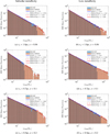 |
Fig. 4 BHMF shift, after stellar feedback expels 99% of the gas, for a gaseous stellar cluster as in Figure 3. In the legend we depict the power exponent, α, of several fits, namely of the BH IMF and of the shifted BHMF for several ranges; the whole range of values, the low-mass range up to the initial PISN cutoff, the range within the upper BH mass gap, and if applicable the tail of heavy BHs. |
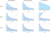 |
Fig. 5 Range of parameters in which the proto-BHMF-shift operates. The rows correspond to different stellar-cluster total masses and the columns to different metallicities. The solid shaded blue region in the ε-rh plane signifies their range in which the most massive BH grows by at least 10 M⊙. The diagonally hatched region signifies additionally the ε-rh range for which an IMBH with a mass of ~103 M⊙ can be generated. Notice that the subsolar and low-metallicity cases require an almost identical cluster compactness for the BHMF-shift to operate, but the solar metallicity case requires about double or higher compactness (x axis). |
BH mass growth, Δm, with respect to the initial mass, m0.
4.2 BHMF-shift thresholds
We investigated the possibility of BHMF shift over a vast range of possible cluster configurations. We ran multiple simulations for three cluster initial total mass values, 105 M⊙, 106 M⊙, and 107 M⊙, for solar, subsolar, and low metallicities, covering the whole ε, rh range. In Figure 5 we depict the range at which our proto-BHMF-shift mechanism operates in the ε-rh plane. The solid filled region designates the conditions in which the initially heavier BH accretes at least 10 M⊙ within our simulation time (up to 99% gas depletion). The diagonally hatched region signifies the range of values in which the formation of an IMBH, with a mass of ~103 M⊙, is possible. The case of M = 106 M⊙ at low metallicity is of special interest. Remarkably, in this case the proto-BHMF shift operates for any ε if rh ≤ 0.6, and equivalently C ≥ 16.67, well within the compactness range of observed proto-stellar clusters, Cobserved ≈ 10–50. This is explained by the form of the depletion timescale diagram 1c. We observe there that the timescale stalls at precisely these compactness values, which are mostly relevant to M = 106 M⊙. The reason for this stall is that energetic PISN explosions operate. Even higher compactness and/or lower ε are not sufficient to increase the timescale within this compactness value range. However, the PISNs proceed fast and if the cluster reaches compactness values that allow it to survive the PISN bursts the timescale increases rapidly. Another interesting feature in this case (low-Z, mass 106 M⊙) is that even at higher rh > 0.6 pc the proto-BHMF shift occurs for both low and high ε. For a fixed depletion timescale, as ε increases the gas component gets more centrally condensed, allowing a similar accretion efficiency with lower ε, which implies more available gas for accretion. This effect does not occur in the rest of the cases because the depletion timescale does not stall. Our analysis shows that a significant BHMF shift is theoretically possible for all metallicities and for clusters with a vast mass range of 105–107 M⊙ as in Figure 5.
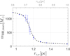 |
Fig. 6 Maximum shifted individual BH mass of an initial 55 M⊙ BH in a stellar cluster with total (stellar) mass M★ = 106 M⊙, for cluster sizes representative of the observed Cosmic Gems proto-stellar clusters. We assumed an initial gas-rich cluster with total M = 3 ∙ 106 M⊙ and star formation efficiency ε = 0.35 at low metallicity. The lower x axis is the final (after gas depletion) Plummer radius, to be compared to the half-light radius of the observed stellar clusters, and the upper x axis is the half-mass radius of the initial gas-rich cluster. |
4.3 Cosmic Gems clusters
We modeled proto-stellar clusters, resembling the observed ones in the Cosmic Gems arc galaxy (Adamo et al. 2024). Their observed masses are in the range of (1–4) ∙ 106 M⊙ and the half-light radii are (0.7–1.7) pc. We adopted ε = 0.35, representing the upper end ~0.3 of observed star formation efficiencies in embedded clusters (Lada & Lada 2003; Baumgardt & Kroupa 2007), appropriate for the extreme densities and low metallicity in such massive, compact proto-stellar clusters as the Cosmic Gems ones. The observations do not allow one to conclusively determine the gas content of the clusters. Their observationally estimated age of 10–50 Myr (Adamo et al. 2024) suggests that they possibly are nearly at the final gas expulsion stage, with little gas remaining. However, the exact amount of gas remaining is uncertain while the galaxy itself is gas-rich. We assumed a low metallicity of 0.01 Z⊙, in accordance with the low metallicity expected for the Cosmic Gems arc galaxy (Adamo et al. 2024).
We chose an initial total mass for the gas-rich cluster of M = 3 ∙ 106 M⊙, which means that M★ = 106 M⊙ for the stellar component, which is at the low-mass end of the observations. In our investigation, we cover a range of initial half-mass radii, rh = 0.6–1 pc, which result in stellar Plummer radii of rc,★ = 0.9–1.6 pc because of expansion due to mass loss. In Figure 6 we depict the maximum individual BH mass with respect to rc,★, to be compared with the observed half-light radius of Cosmic Gems clusters. For all these cluster sizes, the clusters have identical gas depletion timescales, due to the low-Z PISN plateau (Figure 1c),
 (27)
(27)
which implies that by 13 Myr 99% of the gas has been expelled. This is the time at which we terminate the simulations. We find that the upper BH mass gap is populated even for the most conservative cluster sizes, ~1.3–1.6 pc. Remarkably, resulting stellar clusters with rc,★ ≤ 1.15 pc can host IMBHs with masses of ~103 M⊙. In Figure 7 we present the results of ten runs for an initial half-mass radius of rh = 0.72 pc that gives a marginal size of rc,★ = 1.15 pc, which is the maximum radius for which ~103 M⊙ BHs can be formed. This is a conservative value of the observed, effective half-light radii for a ~106 M⊙ Cosmic Gems cluster (see Table 1 of Adamo et al. 2024). The BHMF shifts to higher masses (Figure 7b) populating the mass-gap with a negative power exponent of ≃2.2 fit within the mass-gap range. The power exponent of the tail, mBH > 130 M⊙, is 2.8. There were generated, per cluster, 3082 BHs (based on a stellar Kroupa IMF for progenitor stars), on average constituted of 2928 CCSN-BHs, of which 1320 escape due to recoil kick at birth, 102 are direct-collapse-BHs, and 52 are PPISN-BHs. The BHs accrete on average 4.8 ∙ 104 M⊙ gas mass per cluster (0.6% of the initial gas reservoir). The maximum individual BH mass is 845 M⊙, and occurs for a direct-collapse-BH. The general fit of the individual BH mass increase for all BHs, depicted as a dashed green line in Figure 7a, is ΔmBH = (mBH,birth/23 M⊙)6.7. Excluding the outliers above mass 500 M⊙, the fit becomes ΔmBH = (mBH,birth/20.9 M⊙)5.8. The distinct trends give a power exponent of 7.7 and scale of 26.1 M⊙ for all direct-collapse-BHs and, respectively, 6.4, 18.5 M⊙ for the PPISN-BHs.
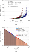 |
Fig. 7 Mass scatter diagram (a), and BHMF (b), for a cluster representing the observed Cosmic Gems proto-stellar clusters, following ten simulation runs. In particular, the initial parameters of the gas-rich cluster are M = 3 ∙ 106 M⊙, rh = 0.72 pc, ε = 0.35, Z ≃ 0.01 Z⊙, and τ = 2.9 Myr, resulting in a stellar cluster after gas is depleted with M★ = 106 M⊙ and rh,★ = 1.15 pc. The general trend of the individual BH mass increase is Δm = (minitial/23 M⊙)67 depicted as the dashed green curve in (a). In (b), α denotes the exponent of each histogram fit. |
4.4 GW231123
Let us discuss the possibility that the BH components of the GW231123 (The LIGO Scientific Collaboration et al. 2025) were generated with our proto-BHMF-shift mechanism in proto-stellar clusters. Their mass ranges,  and
and  , are definitely within the typical proto-BHMF-shift range for a vast range of cluster parameters, including those of Cosmic Gems clusters. However, the critical data that could potentially discriminate between our accretion-driven mass growth in proto-stellar clusters and repeated mergers are the spins of the components BHs estimated as
  and
and  . Notice that these values are higher than the estimated equilibrium value of second-generation repeated mergers with an expected narrow peak at
  (Fishbach et al. 2017) (higher-generation mergers in galactic nuclei could produce higher spins (Yang et al. 2019)). We argue here that these unusually high spin central values of GW231123 are nevertheless consistent with BH spinup due to accretion, especially in the conditions in which our proto-BHMF-shift operates.
Dotti et al. (2013) have shown that BHs with masses of ≲107 M⊙ can maintain high spins, a★ ~ 0.8–0.9, but still below the Thorne limit, 0.998 (Thorne 1974), through chaotic accretion. For this to occur three conditions should be satisfied: (i) multiple randomly oriented accretion episodes, (ii) sufficiently fast BH-disk alignment, and (iii) sufficient disk angular momentum.
In the case of our proto-BHMF-shift mechanism, all three conditions are satisfied. First, since the cluster turbulence has a correlation length of ℓcorr ≈ rh > RB (Bonazzola et al. 1992; Klessen et al. 2000), the time for turbulence and BH displacement to disrupt angular momentum coherence is the time needed for the BH to perform a random walk within rh; that is,  . The accretion timescale is τacc ~ 1–10 Myr depending on local conditions. Multiple randomly oriented accretion events on the order of ~20 should occur for a 100 M⊙ BH. Second, the disk alignment timescale is τalign ≈ 4 ∙ 10–3 Myr ∙ (mBH /100 M⊙)–2/35 (Dotti et al. 2013). This is negligible compared to τacc and also yields τaligh/τdisruption ~ 10–2, allowing for disk alignment before disruption. Finally, since we estimated ~20 realignment episodes, in order for the gas to add significant amount of angular momentum to the BH, the disk angular momentum,
  , should be Jdisk ≳ 0.05 JBH, where
  . Assuming
  and in the cluster’s core ρgas ≃ 106 M⊙/pc3, we get the condition for sufficient angular momentum transfer
  , which means that angular momentum transfer can occur inside the Bondi radius, rout < RB. Therefore, a sufficient amount of gas’ angular momentum can be accumulated within the Bondi radius, especially for an initially low spin of a★ ~ 0.1 and as gas cools down over time.
Thus, we have enough evidence to indicate that the proto-BHMF-shift mechanism can generate a BH with spin at a* ~ 0.8–0.9, consistent with the Dotti et al. (2013) prediction for chaotic accretion onto (low-end) massive BHs. Nevertheless, we plan to investigate in detail the BH spin evolution of BHs with masses of ~50–103 M⊙ within the turbulent environment of a gas-rich proto-stellar cluster in a subsequent work focused on this involved issue.
5 Conclusion
We have calculated the conditions for a gas-rich proto-stellar cluster that can induce a significant BHMF shift, due to accretion. Our analysis includes: detailed calculations of gas depletion timescales incorporating stellar lifetimes, stellar winds, and supernova explosions; the generation of realistic BH populations with assigned progenitor masses; the time-dependent introduction of BHs into the simulation according to their formation times; and the modeling of stochastic perturbations from both gas and stellar components. These elements are crucial for determining the efficiency of BH mass growth over the brief (~ 10–20 Myr in total) simulation times of interest.
Our results identify the specific conditions in which a significant BHMF shift can occur, sufficient at least to populate the upper BH mass gap. At low metallicity with a cluster mass of ~106 M⊙, any star formation efficiency produces shifts if the cluster is sufficiently compact (C > 16.7). For other metallicity, mass, and compactness values, the star formation efficiency is constrained, as is shown in Figure 5. We find that heavy (>150 M⊙) BH tails (like in Figure 4c) and IMBH formation (~103 M⊙) are possible for all compactness values if the star formation efficiency is sufficiently low. Solar metallicity environments require significantly more compactness for the BHMF shift to be effective due to intense stellar winds. As a rule of thumb, the shift in individual BH masses follows a steep power law of ΔmBH ≈ (mBH,birth/20 M⊙)4–6, where the value of the power exponent depends on the compactness, metallicity, and star formation efficiency of the cluster.
This analysis has direct observational implications. The observed Cosmic Gems proto-stellar clusters at high redshift likely experienced early accretion-driven BHMF shifts, generating ≳25 BHs with masses of 102 M⊙ ≲ mBH ≲ 103 M⊙ within their first ≲13 Myr.
Our mechanism can provide further an explanation for some of the heavy, mass-gap BHs (>60 M⊙) detected by LIGO-Virgo-KAGRA. The key element that would allow us to distinguish BHs grown via repeated mergers from the ones grown via accretion is the spin measurement. Chaotic accretion in principle favors low spins. However, in the case in which an accretion disk can align with the BH spin quickly with respect to the timescale of erratic spin reorientation and is also massive enough to transfer significant angular momentum, Dotti et al. (2013) have shown that an equilibrium is reached at a* ~ 0.8–0.9 for massive BHs (≲107 M⊙). This spin is close to the estimated central values of the recent GW231123 signal. Our first estimates (see Section 4.4) suggest that this may also occur for lower-mass BHs (~100 M⊙) in the physical conditions of a gas-rich proto-stellar cluster. However, this requires further investigation with more precise analytical calculations or simulations of BH spin, not performed here.
This work opens several important avenues for future investigation. The “proto-BHMF-shift” mechanism provides a pathway for seeding high-redshift SMBH formation. The IMBHs produced through this channel represent promising targets for GW detection by the future LISA mission. Finally, we plan to investigate the distinctive spin signatures that our mechanism produces in accretion-driven BHs and to develop specific observational predictions to distinguish them from merger-formed BHs in current and future LIGO-Virgo-KAGRA GW data.
Acknowledgements
ZR is supported by the European Union’s Horizon Europe Research and Innovation Programme under the Marie Sklodowska-Curie grant agreement No. 101149270–ProtoBH.
References
- Abbott, R., Abbott, T. D., Acernese, F., et al. 2023, Phys. Rev. X, 13, 041039 [Google Scholar]
- Adamo, A., Bradley, L. D., Vanzella, E., et al. 2024, Nature, 632, 513 [NASA ADS] [CrossRef] [Google Scholar]
- Amaro-Seoane, P., Andrews, J., Arca Sedda, M., et al. 2023, Living Rev. Relat., 26, 2 [Google Scholar]
- Arca Sedda, M., Kamlah, A. W. H., Spurzem, R., et al. 2023, MNRAS, 526, 429 [NASA ADS] [CrossRef] [Google Scholar]
- Atri, P., Miller-Jones, J. C. A., Bahramian, A., et al. 2019, MNRAS, 489, 3116 [NASA ADS] [CrossRef] [Google Scholar]
- Baibhav, V., Gerosa, D., Berti, E., et al. 2020, Phys. Rev. D, 102, 043002 [NASA ADS] [CrossRef] [Google Scholar]
- Bartos, I., & Haiman, Z. 2025, arXiv e-prints [arXiv:2508.08558] [Google Scholar]
- Baumgardt, H., & Kroupa, P. 2007, MNRAS, 380, 1589 [NASA ADS] [CrossRef] [Google Scholar]
- Baumgarte, T. W., & Shapiro, S. L. 2025, Phys. Rev. D, 111, 063039 [Google Scholar]
- Belczynski, K., Heger, A., Gladysz, W., et al. 2016, A&A, 594, A97 [NASA ADS] [CrossRef] [EDP Sciences] [Google Scholar]
- Bestenlehner, J. M., Vink, J. S., Gräfener, G., et al. 2011, A&A, 530, L14 [NASA ADS] [CrossRef] [EDP Sciences] [Google Scholar]
- Bogdán, Á., Goulding, A. D., Natarajan, P., et al. 2024, Nat. Astron., 8, 126 [Google Scholar]
- Bonazzola, S., Perault, M., Puget, J. L., et al. 1992, J. Fluid Mech., 245, 1 [Google Scholar]
- Bonnell, I. A., Clarke, C. J., Bate, M. R., & Pringle, J. E. 2001, MNRAS, 324, 573 [NASA ADS] [CrossRef] [Google Scholar]
- Crowther, P. A. 2007, Ann. Rev. Astron. Astrophys., 45, 177 [Google Scholar]
- Dale, J. E., Ngoumou, J., Ercolano, B., & Bonnell, I. A. 2014, MNRAS, 442, 694 [Google Scholar]
- De Marchi, G., Clampin, M., Greggio, L., et al. 1997, ApJ, 479, L27 [Google Scholar]
- Dessauges-Zavadsky, M., Richard, J., Combes, F., et al. 2019, Nat. Astron., 3, 1115 [NASA ADS] [CrossRef] [Google Scholar]
- Dessauges-Zavadsky, M., Richard, J., Combes, F., et al. 2023, MNRAS, 519, 6222 [NASA ADS] [CrossRef] [Google Scholar]
- Dopita, M. A., & Sutherland, R. S. 2003, Astrophysics of the Diffuse Universe (Springer Nature) [Google Scholar]
- Dotti, M., Colpi, M., Pallini, S., Perego, A., & Volonteri, M. 2013, ApJ, 762, 68 [NASA ADS] [CrossRef] [Google Scholar]
- Ekström, S., Georgy, C., Eggenberger, P., et al. 2012, A&A, 537, A146 [Google Scholar]
- Elmegreen, B. G. 2018, ApJ, 869, 119 [NASA ADS] [CrossRef] [Google Scholar]
- Eswaran, V., & Pope, S. B. 1988, Comput. Fluids, 16, 257 [NASA ADS] [CrossRef] [Google Scholar]
- Federrath, C., Roman-Duval, J., Klessen, R. S., Schmidt, W., & Mac Low, M. M. 2010, A&A, 512, A81 [NASA ADS] [CrossRef] [EDP Sciences] [Google Scholar]
- Fishbach, M., Holz, D. E., & Farr, B. 2017, ApJ, 840, L24 [NASA ADS] [CrossRef] [Google Scholar]
- Frank, J., King, A. R., & Raine, D. J. 1985, Science, 230, 1269 [Google Scholar]
- Fujii, M. S., Wang, L., Tanikawa, A., Hirai, Y., & Saitoh, T. R. 2024, Science, 384, 1488 [NASA ADS] [CrossRef] [Google Scholar]
- Geen, S., Rosdahl, J., Blaizot, J., Devriendt, J., & Slyz, A. 2015, MNRAS, 448, 3248 [Google Scholar]
- Georgy, C., Ekström, S., Eggenberger, P., et al. 2013, A&A, 558, A103 [NASA ADS] [CrossRef] [EDP Sciences] [Google Scholar]
- Gerosa, D., & Berti, E. 2017, Phys. Rev. D, 95, 124046 [NASA ADS] [CrossRef] [Google Scholar]
- Giacobbo, N., & Mapelli, M. 2020, ApJ, 891, 141 [NASA ADS] [CrossRef] [Google Scholar]
- Groh, J. H., Ekström, S., Georgy, C., et al. 2019, A&A, 627, A24 [NASA ADS] [CrossRef] [EDP Sciences] [Google Scholar]
- Guillard, N., Emsellem, E., & Renaud, F. 2016, MNRAS, 461, 3620 [Google Scholar]
- Hamann, W. R., Gräfener, G., & Liermann, A. 2006, A&A, 457, 1015 [NASA ADS] [CrossRef] [EDP Sciences] [Google Scholar]
- Heger, A., & Woosley, S. E. 2002, ApJ, 567, 532 [Google Scholar]
- Heger, A., Fryer, C. L., Woosley, S. E., Langer, N., & Hartmann, D. H. 2003, ApJ, 591, 288 [CrossRef] [Google Scholar]
- Hills, J. G. 1980, ApJ, 235, 986 [NASA ADS] [CrossRef] [Google Scholar]
- Ho, L. C., & Filippenko, A. V. 1996, ApJ, 466, L83 [NASA ADS] [CrossRef] [Google Scholar]
- Hobbs, G., Lorimer, D. R., Lyne, A. G., & Kramer, M. 2005, MNRAS, 360, 974 [Google Scholar]
- Inayoshi, K., Haiman, Z., & Ostriker, J. P. 2016, MNRAS, 459, 3738 [NASA ADS] [CrossRef] [Google Scholar]
- Inayoshi, K., Harikane, Y., Inoue, A. K., Li, W., & Ho, L. C. 2022, ApJ, 938, L10 [NASA ADS] [CrossRef] [Google Scholar]
- Johnson, K. E., Leroy, A. K., Indebetouw, R., et al. 2015, ApJ, 806, 35 [Google Scholar]
- Kasen, D., Woosley, S. E., & Heger, A. 2011, ApJ, 734, 102 [NASA ADS] [CrossRef] [Google Scholar]
- Kimball, C., Talbot, C. L., Berry, C. P., et al. 2020, ApJ, 900, 177 [NASA ADS] [CrossRef] [Google Scholar]
- Klessen, R. S., Heitsch, F., & Mac Low, M.-M. 2000, ApJ, 535, 887 [NASA ADS] [CrossRef] [Google Scholar]
- Krause, M., Fierlinger, K., Diehl, R., et al. 2013, A&A, 550, A49 [NASA ADS] [CrossRef] [EDP Sciences] [Google Scholar]
- Krause, M. G. H., Charbonnel, C., Bastian, N., & Diehl, R. 2016, A&A, 587, A53 [NASA ADS] [CrossRef] [EDP Sciences] [Google Scholar]
- Kroupa, P. 2002, Science, 295, 82 [Google Scholar]
- Kruijssen, J. M. D. 2015, MNRAS, 454, 1658 [Google Scholar]
- Kruijssen, J. M. D., Schruba, A., Chevance, M., et al. 2019, Nature, 569, 519 [NASA ADS] [CrossRef] [Google Scholar]
- Kudritzki, R. P. 2002, ApJ, 577, 389 [NASA ADS] [CrossRef] [Google Scholar]
- Lada, C. J., & Lada, E. A. 2003, Ann. Rev. Astron. Astrophys., 41, 57 [Google Scholar]
- Larson, R. L., Finkelstein, S. L., Kocevski, D. D., et al. 2023, ApJ, 953, L29 [NASA ADS] [CrossRef] [Google Scholar]
- Lee, A. T., & Stahler, S. W. 2011, MNRAS, 416, 3177 [Google Scholar]
- Lee, A. T., & Stahler, S. W. 2014, A&A, 561, A84 [NASA ADS] [CrossRef] [EDP Sciences] [Google Scholar]
- Lee, S., Lee, H. M., Kim, J.-h., et al. 2025, ApJ, 988, 15 [Google Scholar]
- Leigh, N. W. C., Mastrobuono-Battisti, A., Perets, H. B., & Böker, T. 2014, MNRAS, 441, 919 [NASA ADS] [CrossRef] [Google Scholar]
- Leitherer, C., Schaerer, D., Goldader, J. D., et al. 1999, Astrophys. J. Supp., 123, 3 [Google Scholar]
- Mandel, I. 2016, MNRAS, 456, 578 [Google Scholar]
- Mapelli, M., Dall’Amico, M., Bouffanais, Y., et al. 2021, MNRAS, 505, 339 [CrossRef] [Google Scholar]
- McCray, R., & Kafatos, M. 1987, ApJ, 317, 190 [NASA ADS] [CrossRef] [Google Scholar]
- Merritt, D. 2013, Dynamics and Evolution of Galactic Nuclei (Princeton Series in Astrophysics) (Princeton University Press) [Google Scholar]
- Miller, M. C., & Hamilton, D. P. 2002, MNRAS, 330, 232 [Google Scholar]
- Neumayer, N., Seth, A., & Böker, T. 2020, Astron. Astrophys. Rev., 28, 4 [Google Scholar]
- Nomoto, K., Tominaga, N., Umeda, H., Kobayashi, C., & Maeda, K. 2006, Nucl. Phys. A, 777, 424 [CrossRef] [Google Scholar]
- O’Leary, R. M., Rasio, F. A., Fregeau, J. M., Ivanova, N., & O’Shaughnessy, R. 2006, ApJ, 637, 937 [CrossRef] [Google Scholar]
- O’Shaughnessy, R., Gerosa, D., & Wysocki, D. 2017, Phys. Rev. Lett., 119, 011101 [CrossRef] [Google Scholar]
- Ostriker, E. C. 1999, ApJ, 513, 252 [Google Scholar]
- Paczynski, B. 1971, Ann. Rev. Astron. Astrophys., 9, 183 [Google Scholar]
- Parmentier, G., & Pfalzner, S. 2013, A&A, 549, A132 [NASA ADS] [CrossRef] [EDP Sciences] [Google Scholar]
- Perna, R., Wang, Y.-H., Farr, W. M., Leigh, N., & Cantiello, M. 2019, ApJ, 878, L1 [NASA ADS] [CrossRef] [Google Scholar]
- Pittard, J. M. 2019, MNRAS, 488, 3376 [Google Scholar]
- Puls, J., Vink, J. S., & Najarro, F. 2008, Astron. Astrophys. Rev., 16, 209 [Google Scholar]
- Purohit, R. A., Fragione, G., Rasio, F. A., Petter, G. C., & Hickox, R. C. 2024, AJ, 167, 191 [Google Scholar]
- Rahman, N., Janka, H. T., Stockinger, G., & Woosley, S. E. 2022, MNRAS, 512, 4503 [NASA ADS] [CrossRef] [Google Scholar]
- Regan, J., & Volonteri, M. 2024, Open J. Astrophys., 7, 72 [NASA ADS] [CrossRef] [Google Scholar]
- Renzini, A. 2017, MNRAS, 469, L63 [Google Scholar]
- Renzo, M., Ott, C. D., Shore, S. N., & de Mink, S. E. 2017, A&A, 603, A118 [NASA ADS] [CrossRef] [EDP Sciences] [Google Scholar]
- Renzo, M., Cantiello, M., Metzger, B. D., & Jiang, Y. F. 2020, ApJ, 904, L13 [NASA ADS] [CrossRef] [Google Scholar]
- Repolust, T., Puls, J., & Herrero, A. 2004, A&A, 415, 349 [NASA ADS] [CrossRef] [EDP Sciences] [Google Scholar]
- Rizzuto, F. P., Naab, T., Spurzem, R., et al. 2022, MNRAS, 512, 884 [NASA ADS] [CrossRef] [Google Scholar]
- Roupas, Z. 2021, A&A, 646, A20 [NASA ADS] [CrossRef] [EDP Sciences] [Google Scholar]
- Roupas, Z., & Kazanas, D. 2019a, A&A, 621, L1 [NASA ADS] [CrossRef] [EDP Sciences] [Google Scholar]
- Roupas, Z., & Kazanas, D. 2019b, A&A, 632, L8 [NASA ADS] [CrossRef] [EDP Sciences] [Google Scholar]
- Safarzadeh, M., & Haiman, Z. 2020, ApJ, 903, L21 [NASA ADS] [CrossRef] [Google Scholar]
- Sander, A. A. C., & Vink, J. S. 2020, MNRAS, 499, 873 [Google Scholar]
- Schmidt, W., Hillebrandt, W., & Niemeyer, J. C. 2006, Comput. Fluids, 35, 353 [CrossRef] [Google Scholar]
- Sedov, L. I. 1946, J. Appl. Math. Mech., 10, 241 [Google Scholar]
- Shenar, T., Sana, H., Mahy, L., et al. 2022, Nat. Astron., 6, 1085 [NASA ADS] [CrossRef] [Google Scholar]
- Silich, S., Tenorio-Tagle, G., & Muñoz-Tuñón, C. 2003, ApJ, 590, 791 [NASA ADS] [CrossRef] [Google Scholar]
- Spera, M., & Mapelli, M. 2017, MNRAS, 470, 4739 [Google Scholar]
- Spitzer, L. 1987, Dynamical Evolution of Globular Clusters (Princeton University Press) [Google Scholar]
- Sukhbold, T., Ertl, T., Woosley, S. E., Brown, J. M., & Janka, H. T. 2016, ApJ, 821, 38 [NASA ADS] [CrossRef] [Google Scholar]
- Tanaka, T., & Haiman, Z. 2009, ApJ, 696, 1798 [NASA ADS] [CrossRef] [Google Scholar]
- Taylor, G. 1950, Proc. Roy. Soc. Lond. A, 201, 192 [NASA ADS] [CrossRef] [Google Scholar]
- The LIGO Scientific Collaboration, the Virgo Collaboration, & the KAGRA Collaboration 2025, arXiv e-prints [arXiv:2507.08219] [Google Scholar]
- Thorne, K. S. 1974, ApJ, 191, 507 [Google Scholar]
- Torniamenti, S., Mapelli, M., Périgois, C., et al. 2024, A&A, 688, A148 [NASA ADS] [CrossRef] [EDP Sciences] [Google Scholar]
- Vanzella, E., Caminha, G. B., Calura, F., et al. 2020, MNRAS, 491, 1093 [Google Scholar]
- Vink, J. S. 2017, Philos. Trans. Roy. Soc. Lond. A, 375, 20160269 [Google Scholar]
- Vink, J. S., de Koter, A., & Lamers, H. J. G. L. M. 2001, A&A, 369, 574 [NASA ADS] [CrossRef] [EDP Sciences] [Google Scholar]
- Watkins, E. J., Kreckel, K., Groves, B., et al. 2023, A&A, 676, A67 [NASA ADS] [CrossRef] [EDP Sciences] [Google Scholar]
- Woosley, S. E. 2017, ApJ, 836, 244 [Google Scholar]
- Woosley, S. E., & Heger, A. 2021, ApJ, 912, L31 [NASA ADS] [CrossRef] [Google Scholar]
- Woosley, S. E., & Weaver, T. A. 1995, Astrophys. J. Supp., 101, 181 [Google Scholar]
- Yang, Y., Bartos, I., Gayathri, V., et al. 2019, Phys. Rev. Lett., 123, 181101 [CrossRef] [Google Scholar]
- Zick, T. O., Weisz, D. R., & Boylan-Kolchin, M. 2018, MNRAS, 477, 480 [Google Scholar]
All Tables
All Figures
|
Fig. 1 Our estimated depletion timescale, τ, with respect to the compactness, C, of a gaseous stellar cluster of any total mass. We considered three possible star formation efficiencies, ε. Each sub-figure (a), (b), (c) corresponds, respectively, to solar, subsolar (~0.1 Z⊙), and low (~0.01 Z⊙) metallicity. We assume that at subsolar metallicity PPISN operates, and that in the low-metallicity case both PPISN and PISN do. |
| In the text | |
|
Fig. 2 BH-remnant mass with respect to the ZAMS progenitor’s mass, reproduced from Spera & Mapelli (2017), used here in determining the BH entry time in our simulation. |
| In the text | |
|
Fig. 3 Shifted BH masses, after stellar feedback expels 99% of the gas, with respect to the initial BH masses for a gaseous stellar cluster with total initial mass M = 106 M⊙ containing ~1000 BHs, for several star formation efficiency and half-mass radius, i.e., compactness, values of the cluster. Each subfigure was generated by a set of ten simulations. The left column corresponds to subsolar metallicity (~0.1 Z⊙), the right column to low metallicity (~0.01 Z⊙). The solar metallicity case, not shown here, requires about double or higher compactness to have the same effect as the subsolar case. |
| In the text | |
|
Fig. 4 BHMF shift, after stellar feedback expels 99% of the gas, for a gaseous stellar cluster as in Figure 3. In the legend we depict the power exponent, α, of several fits, namely of the BH IMF and of the shifted BHMF for several ranges; the whole range of values, the low-mass range up to the initial PISN cutoff, the range within the upper BH mass gap, and if applicable the tail of heavy BHs. |
| In the text | |
|
Fig. 5 Range of parameters in which the proto-BHMF-shift operates. The rows correspond to different stellar-cluster total masses and the columns to different metallicities. The solid shaded blue region in the ε-rh plane signifies their range in which the most massive BH grows by at least 10 M⊙. The diagonally hatched region signifies additionally the ε-rh range for which an IMBH with a mass of ~103 M⊙ can be generated. Notice that the subsolar and low-metallicity cases require an almost identical cluster compactness for the BHMF-shift to operate, but the solar metallicity case requires about double or higher compactness (x axis). |
| In the text | |
|
Fig. 6 Maximum shifted individual BH mass of an initial 55 M⊙ BH in a stellar cluster with total (stellar) mass M★ = 106 M⊙, for cluster sizes representative of the observed Cosmic Gems proto-stellar clusters. We assumed an initial gas-rich cluster with total M = 3 ∙ 106 M⊙ and star formation efficiency ε = 0.35 at low metallicity. The lower x axis is the final (after gas depletion) Plummer radius, to be compared to the half-light radius of the observed stellar clusters, and the upper x axis is the half-mass radius of the initial gas-rich cluster. |
| In the text | |
|
Fig. 7 Mass scatter diagram (a), and BHMF (b), for a cluster representing the observed Cosmic Gems proto-stellar clusters, following ten simulation runs. In particular, the initial parameters of the gas-rich cluster are M = 3 ∙ 106 M⊙, rh = 0.72 pc, ε = 0.35, Z ≃ 0.01 Z⊙, and τ = 2.9 Myr, resulting in a stellar cluster after gas is depleted with M★ = 106 M⊙ and rh,★ = 1.15 pc. The general trend of the individual BH mass increase is Δm = (minitial/23 M⊙)67 depicted as the dashed green curve in (a). In (b), α denotes the exponent of each histogram fit. |
| In the text | |
Current usage metrics show cumulative count of Article Views (full-text article views including HTML views, PDF and ePub downloads, according to the available data) and Abstracts Views on Vision4Press platform.
Data correspond to usage on the plateform after 2015. The current usage metrics is available 48-96 hours after online publication and is updated daily on week days.
Initial download of the metrics may take a while.