| Issue |
A&A
Volume 702, October 2025
|
|
|---|---|---|
| Article Number | L19 | |
| Number of page(s) | 6 | |
| Section | Letters to the Editor | |
| DOI | https://doi.org/10.1051/0004-6361/202557034 | |
| Published online | 28 October 2025 | |
Letter to the Editor
Direct measurements of the speed of gravitational waves using the Decihertz Interferometer Gravitational Wave Observatory
1
Institute for Frontiers in Astronomy and Astrophysics, Beijing Normal University, Beijing 102206, China
2
School of Physics and Astronomy, Beijing Normal University, Beijing 100875, China
3
Instituto de Física Téorica UAM-CSIC, Universidad Autónoma de Madrid 28049, Spain
4
School of Physics and Optoelectronic, Yangtze University, Jingzhou 434023, China
5
National Centre for Nuclear Research, Pasteura 7, 02-093 Warsaw, Poland
6
Department of Physics, Nagoya University, Nagoya, Aichi 464-8602, Japan
⋆ Corresponding authors: This email address is being protected from spambots. You need JavaScript enabled to view it.
; This email address is being protected from spambots. You need JavaScript enabled to view it.
; This email address is being protected from spambots. You need JavaScript enabled to view it.
Received:
29
August
2025
Accepted:
7
October
2025
Abstract
In this Letter, we propose a new model-independent strategy for a direct measurement of the speed of gravitational waves vg based on the DECi-hertz Interferometer Gravitational-wave Observatory (DECIGO), a future Japanese space gravitational-wave antenna. Our methodology leverages DECIGO’s ability to measure the cosmological distance DL(z) and the cosmic expansion rate H(z) at the same redshift. Each binary neutron star (BNS) inspiral creates a valuable opportunity for a direct measurement of the speed of gravitational waves (GWs) at different redshifts and directions in the sky. In the DECIGO low-frequency band, observation of BNSs during a one-year mission would produce robust measurements of the absolute value of vg with an accuracy at the 10−5 level. Such assessments of vg in the low-frequency domain improve by three orders of magnitude over other direct methods based on ground-based GW detectors (in the high-frequency domain). If General Relativity is not the ultimate theory of gravity, DECIGO will provide the evidence of its failure through a one-year observation of BNS events.
Key words: gravitational waves
© The Authors 2025
 Open Access article, published by EDP Sciences, under the terms of the Creative Commons Attribution License (https://creativecommons.org/licenses/by/4.0), which permits unrestricted use, distribution, and reproduction in any medium, provided the original work is properly cited.
This article is published in open access under the Subscribe to Open model. This email address is being protected from spambots. You need JavaScript enabled to view it. to support open access publication.
1. Introduction
The first direct detection of the gravitational wave (GW) source GW150914 opened an era of GW astronomy and added a new dimension to multi-messenger astrophysics (Abbott et al. 2016). Inspiraling binary neutron stars (BNS) are promising sources to be used as standard sirens (Abbott et al. 2017a), provided their host galaxies can be identified and their associated redshift are measured (Schutz 1986). More importantly, as GW detectors are operational and gathering data, it will be possible to test various aspects of General Relativity (GR) in a ways inaccessible to other techniques. For example, the speed of GWs has been measured using the time delay among GW detectors (Cornish et al. 2017) and the time delay between GW and electromagnetic observations (Abbott et al. 2017b). However, alternative theories of gravity predict vg ≠ c due to the breaking of the weak equivalence principle or the existence of massive gravitons (Will 2005). In this Letter, we focus on a new approach to directly measuring vg with the DECi-hertz Interferometer Gravitational-wave Observatory (DECIGO), a proposed Japanese space mission based on laser interferometer space satellites (Kawamura et al. 2011). We stress that the 0.1–10 Hz frequency band covered by DECIGO will fill the gap between LISA and ground-based detectors, thereby expanding the reach of nascent GW astronomy (Yagi et al. 2012; Cao et al. 2021, 2022). In particular, it will be possible to detect and follow the last stages of BNSs during the low-frequency adiabatic inspiral phase long before their final coalescence. This opens up the possibility for measuring the speed of GWs in the distant universe, especially in the 0.1–1 Hz band, which DECIGO is most sensitive to. In the context of the accelerating expansion of the Universe, effective field theories (EFT) provide a powerful theoretical framework to incorporate an additional scalar field to describe the dynamics of the universe and its possible couplings to gravity (Chen et al. 2015). In some EFT models (Joyce et al. 2015), transient deviations of vg from the speed of light are allowed at frequencies well below ground-based detectors. Note that the massive graviton scenario can also lead to a frequency-dependent GW propagation speed (Ezquiaga et al. 2021), which is testable in any theory of gravity where the spectral dimension of spacetime changes with the probed scale (Yunes et al. 2016). The advantages of our method are the following. (I) It offers the first empirical assessment of the speed of GWs at times much earlier than the present. (II) Testing the consistency of vg measurements across different redshifts and sky positions would be an important test of GR. (III) Measuring vg(flow) at different frequencies, which is nearly impossible at the present stage, would be of paramount importance for probing the landscape of dark energy and extended gravitational models. Throughout this analysis, we denote the speed of light by c and adopt a notation, c0 = 299792.458 km s−1, for its laboratory-measured value, which is also supported by recent astrophysical observations (Cao et al. 2017, 2020; Liu et al. 2021).
2. Methodology and simulation
Our proposed method, based on the theoretical framework described in Baker et al. (2022), relies on the ability of future GW interferometers to measure the luminosity distance DL(z) and the expansion rate H(z). From the DL(z), its derivative, and the expansion rate, it is possible to calculate the speed of GWs (vg) (see Appendix A). DECIGO is the only proposed future detector that could achieve such a scientific goal (Seto et al. 2001). Compared to other ground-based and space-based GW detectors (Hou et al. 2025), the advantage of DECIGO lies in its ability to register a much larger number of GW cycles from BNSs, even at a redshift of z ∼ 5 (Kawamura et al. 2019). This would enable the discovery of a larger number of BNSs in their inspiral phase long before entering the frequency range of Laser Interferometer Gravitational-Wave Observatory (LIGO) (Kawamura et al. 2019). Therefore, the signal-to-noise ratio (S/N) of DECIGO is much higher than that of current ground-based GW detectors, so the measurement uncertainty of DL(z) will be considerably reduced. In addition to the luminosity distance, we still need to assess the expansion rate, and the redshift-drift measurement meets our demands. It is given by the following expression:  , where Δt0 and H0 denote the observation period and the Hubble constant, respectively (Loeb 1998). To follow, the Hubble parameter at redshift z can be written as
 (1)
(1)
The order of magnitude of the redshift drift is roughly given as the observation time divided by the cosmic age, which makes it difficult to measure Δtz with current technology (Yoo et al. 2011). On the other hand, DECIGO is the only proposed detector that can precisely measure a GW phase correction Ψacc(f) due to cosmic acceleration. The Fourier transform of the GW waveform from a coalescing binary system of masses m1 and m2 can be expressed as
![Mathematical equation: $$ \begin{aligned} \tilde{h}(f) \big |_{\text{ no} \text{ accel}} =\frac{\sqrt{3}}{2}\mathcal{A} f^{-7/6}e^{i\Psi (f)} \left[ \frac{5}{4}A_{\mathrm{pol} ,\alpha }(t(f)) \right] e^{-i \left( \varphi _{\mathrm{pol} ,\alpha }+\varphi _D \right) }. \end{aligned} $$](/articles/aa/full_html/2025/10/aa57034-25/aa57034-25-eq3.gif) (2)
(2)
The amplitude of the GW is
 (3)
(3)
where the redshifted chirp mass, ℳz = (1 + z)η3/5Mt, is related to the total mass, Mt = m1 + m2, and the symmetric mass ratio, η = m1m2/Mt2. The function Ψ(f) represents the frequency-dependent phase arising from the orbital evolution, which can be given by the second post-Newtonian (2-PN) approximation (Maggiore 2008b). The polarisation amplitude Apol, α(t), the polarisation phases φpol, α(t) (α represents the number of individual detectors), and the Doppler phase φD(t) are explicitly given in Yagi & Tanaka (2010).
One of the main objectives of DECIGO would be to directly measure the accelerated expansion of the Universe (Yagi et al. 2012). This is possible by measuring GWs coming from BNSs at far distances, since the phase of the waveform can shift if the sources recede due to acceleration. Let us first derive the correction to the GW phase caused by the accelerating expansion of the universe. We define h(Δt) as the observed GW waveform, where Δt = tc − t denotes the time to coalescence measured in the observer’s frame with tc representing the coalescence time. In our method, time to coalescence is equivalent to Δto used in Eq. (1). To follow, Δt can be related to ΔT ≡ (1 + zc)Δte as (Takahashi & Nakamura 2005)
 (4)
(4)
where zc is the source redshift at coalescence, Δte is the time to coalescence measured in the source frame, and X(z) is the acceleration parameter defined as  . In Friedmann-Lemaître-Robertson-Walker (FLRW) space-time, X(z) is related to the redshift drift expressed as Δtz = 2(1 + z)ΔtoX(z). The Fourier component of this waveform is
 (5)
(5)
with
 (6)
(6)
where x = (πℳzf)2/3,  and
and  corresponds to the gravitational waveform in the Fourier domain without cosmic acceleration. A term proportional to x−n represents the n-th PN order relative to the leading Newtonian phase ΨN(f); hence, this is a ‘4-PN’ correction. This means that lower-frequency GWs detectable with DECIGO are advantageous (Quartin & Amendola 2010). The measurement accuracy of X(z) has been estimated in Seto et al. (2001), using the so-called ultimate DECIGO, which is three orders of magnitude more sensitive than the realistic DECIGO detector (Takahashi & Nakamura 2005). The influence of the line-of-sight contamination could affect the phase shift measurement due to a weak lensing effect, especially for high-redshift GWs (Takahashi 2004). Therefore, we limit the following analysis to the redshift range z ≲ 2.0. We estimated the measurement accuracy of the parameter XH ≡ X(z)/H0, using deep learning techniques, based on the one-side noise power spectral density Sh(f) characterising the performance of the realistic GW detector (Yagi et al. 2011; Kawamura et al. 2019). The crucial part of our idea is to perform separate analyses in the low- and high-frequency bands for each BNS observed at redshift z. Let us now describe the division between these bands in more detail. Regarding the low-frequency band, the initial frequency registered, i.e. the frequency at Δto before the coalescence, is fixed at fin = (256/5)−3/8π−1ℳz−5/8Δto−3/8, while the final frequency of this band is fixed at ffin = 1/(1 + z)Hz, in order to guarantee a constant value of vg(f) from the source to the observer (see Eq. (13) in Appendix A). In the high-frequency band, the initial frequency is fixed at fin = 1 Hz, while the final cut-off frequency is taken as ffin = 100 Hz, DECIGO’s higher frequency (Yagi & Tanaka 2010).
The waveform analysis allows us to fit the following parameter vector  , where β denotes the spin-orbit coupling parameter and ϕc is the coalescence phase. (θS, ϕS) and (θL, ϕL) denote, respectively, the direction of the source and the orientation of its orbital axis in the barycentric frame. In our simulations we set the fiducial values of m1 = m2 = 1.4 M⊙ and tc = ϕc = β = 0 without losing generality (Yagi & Tanaka 2010). Considering DECIGO’s angular resolution (∼arcsec2), which can uniquely identify the host galaxy of the binary, it is possible to determine the angular position (θS, ϕS) by pointing telescopes towards the location uncertainty box at the expected coalescence time from the chirp signal (Kawamura et al. 2019). We perform a Monte Carlo simulation by randomly distributing the orientation of sources (θL, ϕL). The effect of modified gravity θMG is quantified by two parameters: the transition frequency ftrans and the height of the vg transition δvg = vg(fhigh)−vg(flow). In our analysis the exact location of the transition frequency is not included as a free parameter to be fitted, provided that it lies between the low- and high-frequency bands of DECIGO (Baker et al. 2023). The uncertainties of DL(z) and H(z) were estimated using a convolutional neural network (CNN), the network structure of which has been presented in detail in Sun et al. (2024, see our Appendix B). Since DECIGO is expected to detect BNS mergers at a rate of ∼104 yr−1 (Seto et al. 2001), two observational strategies were applied in the simulations: (Strategy I) a one-month observation of 103 BNS, and (Strategy II) a one-year observation of 104 BNS. The merger rate of double compact objects in a cosmological scenario is quantified by the conservative star formation rate (SFR) function (Dominik et al. 2013). We employed Gaussian processes (GP) to extract information from DL(z) and its related errors σDL, which yield numerically reconstructed DL(z) and D′L(z) as smooth analytical functions (Seikel et al. 2012). Then, we evaluated the GP output function on the individual H(z) measurements, with the output of vg(z) at different redshifts.
3. Numerical results and implication
We applied the techniques outlined above to the two observational strategies of DECIGO, focusing on the low-frequency and high-frequency GW signals from the BNS. A fiducial flat ΛCDM cosmology is applied, with Ωm = 0.30 and H0 = 70 km/s/Mpc. Our results show that tighter constraints on the speed of GWs are obtained in the low-frequency band, since the effect due to cosmic acceleration is greater on GW signals with lower frequencies (Seto et al. 2001; Kawamura et al. 2019). In order to analyse the performance of our method, we considered two scenarios, where the height of the transition δvg(flow)/c0 = 10−4 and δvg(flow)/c0 = 10−5, respectively, occurring at f = 1Hz (Baker et al. 2023). The results for both observational strategies are presented in Fig. 1. As shown, DECIGO will provide reasonably precise measurements of GW speeds from sources located at different redshifts. By benefiting from the accumulation of a large number of inspiral cycles in registered GW signals, which enables high-precision measurements of the phase shift associated with the redshift drift, such a space-based GW detector will more precisely measure DL(z) and H(z), resulting in better measurements of vg(flow) at different redshifts. Disagreement between such individual vg(z) measurements, if statistically significant, could be a probe of GR, considering modifications of the group velocity of GWs generated by Lorentz invariance violation in the gravity sector of the gravitational Standard-Model Extension (Kostelecký & Mewes 2016).
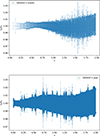 |
Fig. 1. Measurements of the speed of GWs based on a one-month (upper panel) and a one-year (lower panel) observation of BNS events by DECIGO. The scale of departure from the GR δvg(flow)/c0 is assumed to be 10−4 and 10−5, respectively. |
When we summarised multiple vg(flow) measurements through the inverse variance weighting, the final constraint with 1σ uncertainty is vg(flow)/c0 = 0.9997 ± 0.0005 for strategy I. This means that the one-month long observation enabled testing deviations of δvg(flow)/c0 from zero (as predicted by GR) with a precision of 5 × 10⁻⁴. Hence, the fiducial transition height δvg(flow)/c0 = 10−4 underlying the simulations of strategy I could be detected. It is also clear that a one-month observation by DECIGO would not be sufficient to detect a δvg(flow)/c0 = 10−5 deviation, even if the GR were not the correct theory of gravity. We then proceeded by exploring whether a one-year observation of DECIGO could perform better. Summarising multiple vg(flow) measurements through the inverse variance weighting, the final constraint with 1σ uncertainty results in vg(flow)/c0 = 0.99997 ± 0.00005. Therefore, if the speed GWs at low frequencies differs from c0 by a factor of 10−5, DECIGO will succeed in detecting the signal of GR failure through a one-year observation of BNS events. Figure 2 gives us insight into the performance of our method and its relation to alternative methods of direct measurements of the speed of GWs. It should be stressed that we consider the propagation of GWs in an expanding universe under the far-field approximation. This assumption is equally valid for both flow and fhigh frequency limits relevant to our study. If the graviton is massive, it may cause backreaction on the source, which in turn could imprint timing uncertainties in measuring the vg variation during later propagation (de Rham et al. 2011). However, the uncertainty or lacking information in the vg variation near the source will not affect the conclusions derived from our simulations (see Appendix C for further discussion).
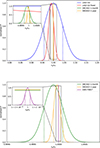 |
Fig. 2. Posterior distributions of vg determined by different techniques. DECIGO data under observing strategies I (one-month) and II (one-year) are compared with two other methods: a direct method based on transit time across a separated network of detectors, and an indirect method using the time delay of GW170817. Two strategies were considered: LIGO O2 – data from O2 of Advanced LIGO-Virgo – and LIGO O2 fixed – where the sky localization of the BNS source is fixed. Note that LIGO O2 and GW170817 only provide constraints on vg/c, and at low redshifts, we take c = c0 in this figure. |
It would be appropriate to compare the above bounds with the recent observational studies of GWs. For example, Liu et al. (2020) proposed a method of determining the speed of GWs by measuring the transit time across a geographically separated network of detectors. By combing ten binary black hole (BBH) events and the BNS event from the second observing run of Advanced LIGO and Advanced Virgo, they constrained the speed of GWs as vg(fhigh)/c0 to (0.97c, 1.05c). Such speed was narrowed down to (0.97c, 1.01c) by fixing the sky localization of the BNS source at the electromagnetic (EM) counterpart. This is actually another way to indirectly measure the speed of GWs. As clearly seen from the vg assessment comparison between DECIGO and Advanced LIGO + Advanced Virgo, the second generation space-based GW detector will result in more stringent constraints on vg. Moreover, very strong constraints on the difference between the speed of gravity and the speed of light (−3 × 10⁻¹⁵ < δtvg(fhigh)/c < +7 × 10⁻¹⁶) have also been obtained using the time delay between GW and EM observations of GW170817 (Abbott et al. 2017b). Since this result exceeds the yields of our method by orders of magnitude, some comments are in order. First, the bound relies on the particular interpretation of the time delay Δt = 1.74 ± 0.05s between the coalescence moment registered in GW band and the peak of gamma-ray fluence (Ciolfi & Siegel 2014). Relaxing model assumptions about the EM emission, or including certain exotic scenarios for the time difference could lead reduce the precision by two orders of magnitude (Abbott et al. 2017b). Moreover, this indirect method, which measures vg relative to c at a specific redshift, depends on the prior assumption that c is constant. These effects would significantly reduce the effectiveness of time-delay based measurements, assuming much smaller numbers of associated BNS-GRB events probed at higher redshifts (Sathyaprakash et al. 2010). Moreover, our method offers a direct measurement of the speed of GWs - the only one proposed besides the time differences between detectors in the network. On the one hand, assuming additional BNS events observed at different redshifts and directions in the sky, the combination of both direct and indirect vg measurements will place limits on the anisotropy of the speed of gravity. On the other hand, assessing vg(flow) from our analysis is of paramount importance for probing the different speed of GWs at high and low frequencies, which are nearly inaccessible at the present stage of GW astrophysics.
Acknowledgments
We thank Prof. Jin Li and Dr. Mengfei Sun for helpful discussion. This work is supported by Beijing Natural Science Foundation No. 1242021, National Natural Science Foundation of China (Nos. 12021003, 12433001); and the Fundamental Research Funds for Central Universities.
References
- Abbott, B. P., Abbott, R., Abbott, T. D., et al. 2016, Phys. Rev. Lett., 116, 061102 [Google Scholar]
- Abbott, B. P., Abbott, R., Abbott, T. D., et al. 2017a, Phys. Rev. Lett., 119, 161101 [Google Scholar]
- Abbott, B. P., Abbott, R., Abbott, T. D., et al. 2017b, ApJ, 848, L13 [CrossRef] [Google Scholar]
- Abbott, B. P., Abbott, R., Abbott, T. D., et al. 2017c, Phys. Rev. Lett., 118, 221101 [CrossRef] [Google Scholar]
- Alsing, J., Silva, H. O., & Berti, E. 2018, MNRAS, 478, 1377 [NASA ADS] [CrossRef] [Google Scholar]
- Amelino-Camelia, G. 2002, Nature, 418, 34 [Google Scholar]
- Amendola, L., Balbi, A., & Quercellini, C. 2008, Phys. Lett. B, 660, 81 [Google Scholar]
- Baker, T., Calcagni, G., Chen, A., et al. 2022, JCAP, 2022, 031 [CrossRef] [Google Scholar]
- Baker, T., Barausse, E., Chen, A., et al. 2023, JCAP, 2023, 044 [CrossRef] [Google Scholar]
- Belgacem, E., Calcagni, G., Crisostomi, M., et al. 2019, JCAP, 2019, 024 [CrossRef] [Google Scholar]
- Brans, C., & Dicke, R. H. 1961, Phys. Rev., 124, 925 [NASA ADS] [CrossRef] [Google Scholar]
- Cao, S., Biesiada, M., Jackson, J., et al. 2017, JCAP, 2017, 012 [CrossRef] [Google Scholar]
- Cao, S., Qi, J., Cao, Z., et al. 2019, Sci. Rep., 9, 11608 [NASA ADS] [CrossRef] [Google Scholar]
- Cao, S., Qi, J., Biesiada, M., Liu, T., & Zhu, Z.-H. 2020, ApJ, 888, L25 [Google Scholar]
- Cao, S., Qi, J., Biesiada, M., et al. 2021, MNRAS, 502, L16 [NASA ADS] [CrossRef] [Google Scholar]
- Cao, S., Qi, J., Cao, Z., et al. 2022, A&A, 659, L5 [NASA ADS] [CrossRef] [EDP Sciences] [Google Scholar]
- Chen, Y., Geng, C.-Q., Cao, S., Huang, Y.-M., & Zhu, Z.-H. 2015, JCAP, 2015, 010 [Google Scholar]
- Christensen, N., & Meyer, R. 2022, Rev. Mod. Phys., 94, 025001 [NASA ADS] [CrossRef] [Google Scholar]
- Ciolfi, R., & Siegel, D. M. 2014, ApJ, 798, L36 [Google Scholar]
- Cornish, N., Blas, D., & Nardini, G. 2017, Phys. Rev. Lett., 119, 161102 [Google Scholar]
- Cutler, C., & Flanagan, E. E. 1994, Phys. Rev. D, 49, 2658 [Google Scholar]
- de Rham, C., Gabadadze, G., & Tolley, A. J. 2011, Phys. Rev. Lett., 106, 231101 [CrossRef] [Google Scholar]
- Dominik, M., Belczynski, K., Fryer, C., et al. 2013, ApJ, 779, 72 [Google Scholar]
- Dreissigacker, C., Sharma, R., Messenger, C., Zhao, R., & Prix, R. 2019, Phys. Rev. D, 100, 044009 [NASA ADS] [CrossRef] [Google Scholar]
- Edwards, M. C. 2021, Phys. Rev. D, 103, 024025 [NASA ADS] [CrossRef] [Google Scholar]
- Ezquiaga, J. M., Hu, W., Lagos, M., & Lin, M.-X. 2021, JCAP, 2021, 048 [CrossRef] [Google Scholar]
- George, D., & Huerta, E. A. 2018, Phys. Lett. B, 778, 64 [NASA ADS] [CrossRef] [Google Scholar]
- Hou, S., Zhao, Z.-C., Cao, Z., & Zhu, Z.-H. 2025, Chin. Phys. Lett., 42, 101101 [Google Scholar]
- Joyce, A., Jain, B., Khoury, J., & Trodden, M. 2015, Phys. Rep., 568, 1 [NASA ADS] [CrossRef] [Google Scholar]
- Kawamura, S., Nakamura, T., Ando, M., et al. 2006, Class. Quant. Grav., 23, S125 [NASA ADS] [CrossRef] [Google Scholar]
- Kawamura, S., Ando, M., Seto, N., et al. 2011, Class. Quant. Grav., 28, 094011 [CrossRef] [Google Scholar]
- Kawamura, S., Nakamura, T., Ando, M., et al. 2019, Int. J. Mod. Phys. D, 28, 1845001 [NASA ADS] [CrossRef] [Google Scholar]
- Kostelecký, A. V., & Mewes, M. 2016, Phys. Lett. B, 510 [Google Scholar]
- Landry, P., & Read, J. S. 2021, ApJ, 921, L25 [NASA ADS] [CrossRef] [Google Scholar]
- Liu, X., He, V. F., Mikulski, T. M., et al. 2020, Phys. Rev. D, 102, 024028 [Google Scholar]
- Liu, T., Cao, S., Biesiada, M., et al. 2021, MNRAS, 506, 2181 [NASA ADS] [CrossRef] [Google Scholar]
- Loeb, A. 1998, ApJ, 499, L111 [NASA ADS] [CrossRef] [Google Scholar]
- Maggiore, M. 2008a, Class. Quant. Grav., 25, 1667 [Google Scholar]
- Maggiore, M. 2008b, Gravitational Waves (New York: Oxford University Press) [Google Scholar]
- Mirshekari, S., Yunes, N., & Will, C. M. 2012, Phys. Rev. D, 85, 024041 [Google Scholar]
- Planck Collaboration VI. 2020, A&A, 641, A6 [NASA ADS] [CrossRef] [EDP Sciences] [Google Scholar]
- Qi, J., Cao, S., Biesiada, M., et al. 2019, Phys. Rev. D, 100, 023530 [NASA ADS] [CrossRef] [Google Scholar]
- Quartin, M., & Amendola, L. 2010, Phys. Rev. D, 81, 043522 [Google Scholar]
- Salzano, V. 2017, Phys. Rev. D, 95, 084035 [Google Scholar]
- Sathyaprakash, B. S., Schutz, B. F., & Van Den Broeck, C. 2010, Class. Quant. Grav., 27, 215006 [NASA ADS] [CrossRef] [Google Scholar]
- Schutz, B. F. 1986, Nature, 323, 310 [Google Scholar]
- Sefiedgar, A. S., Nozari, K., & Sepangi, H. R. 2011, Phys. Lett. B, 696, 119 [Google Scholar]
- Seikel, M., Clarkson, C., & Smith, M. 2012, JCAP, 2012, 036 [CrossRef] [Google Scholar]
- Seto, N., Kawamura, S., & Nakamura, T. 2001, Phys. Rev. Lett., 87, 221103 [Google Scholar]
- Sun, M., Li, J., Cao, S., & Liu, X. 2024, A&A, 682, A177 [NASA ADS] [CrossRef] [EDP Sciences] [Google Scholar]
- Takahashi, R. 2004, A&A, 423, 787 [NASA ADS] [CrossRef] [EDP Sciences] [Google Scholar]
- Takahashi, R., & Nakamura, T. 2005, Prog. Theor. Phys., 113, 63 [Google Scholar]
- Uzan, J.-P., Bernardeau, F., & Mellier, Y. 2008, Phys. Rev. D, 77, 021301 [Google Scholar]
- Will, C. M. 2005, in 100 Years of Relativity, ed. A. Ashtekar, 205 [Google Scholar]
- Yagi, K., & Tanaka, T. 2010, Phys. Rev. D, 81, 064008 [Google Scholar]
- Yagi, K., Tanahashi, N., & Tanaka, T. 2011, Phys. Rev. D, 83, 084036 [NASA ADS] [CrossRef] [Google Scholar]
- Yagi, K., Nishizawa, A., & Yoo, C.-M. 2012, JCAP, 2012, 031 [Google Scholar]
- Yoo, C.-M., Kai, T., & Nakao, K.-I. 2011, Phys. Rev. D, 83, 043527 [Google Scholar]
- You, Z.-Q., Zhu, X., Liu, X., et al. 2025, Nat. Astron., 9, 552 [Google Scholar]
- Yunes, N., Yagi, K., & Pretorius, F. 2016, Phys. Rev. D, 94, 084002 [NASA ADS] [CrossRef] [Google Scholar]
Appendix A: Theoretical framework of GW speed
In this appendix we introduce the general theoretical framework of frequency-dependent vg(f) and its corresponding observables that were used in this Letter. This framework has been developed in the LISA science papers regarding tests of modified gravity theories with the future GW space-detectors (Baker et al. 2022). See Baker et al. (2023) for a comprehensive discussion of the speed of GWs in modified gravity theories. It has been shown that a non-trivial speed of GWs, affects both the phase and the amplitude of the signal from a coalescing binary, hence affecting the GW luminosity distance (Belgacem et al. 2019). Furthermore, the expression of the luminosity distance measured with GWs as a function of redshift is also affected by a non-trivial speed of GWs.
Specifically, a quadratic action for the linearised transverse-traceless GW modes was considered (Baker et al. 2022)
![Mathematical equation: $$ \begin{aligned} S_T\,=\,\frac{ M_{\rm Pl}^2}{8} \,\int d t\,d^3 x\;a^3(t)\,\bar{\alpha }\,\left[ \dot{h}_{ij}^2- \frac{v_g^2 (f)}{a^2(t)} (\boldsymbol{\nabla }h_{ij})^2 \right], \end{aligned} $$](/articles/aa/full_html/2025/10/aa57034-25/aa57034-25-eq12.gif) (A.1)
(A.1)
where MPl denotes the reduced Planck mass. This framework describes free GWs travelling freely in a flat FLRW metric (Qi et al. 2019; Cao et al. 2019)
![Mathematical equation: $$ \begin{aligned} d s^2\,=\, v_g(f)\,\bar{\alpha }\left[-v_g^2(f)\,d t^2+a^2(t)\, d \boldsymbol{x}^2\right] \,. \end{aligned} $$](/articles/aa/full_html/2025/10/aa57034-25/aa57034-25-eq13.gif) (A.2)
(A.2)
with arbitrary speed of vg(f). This is an effective metric which LISA Cosmology Working Group use for describing the propagation of the GW (Belgacem et al. 2019), with the Lagrangian density for a free spin-2 field (in the integrand of Eq. (A.1))
![Mathematical equation: $$ \begin{aligned} { L}_T&= \sqrt{-\tilde{g}} \left[ \tilde{g}^{\mu \nu } \partial _\mu h_{ij}\partial _\nu h_{ij} \right] \\ \nonumber&= a^3\,\bar{\alpha }\, \left[ \dot{h}_{ij}^2-\frac{v_g^2 }{a^2} \left( boldsymbol{\nabla }h_{ij} \right)^2 \right]\,. \end{aligned} $$](/articles/aa/full_html/2025/10/aa57034-25/aa57034-25-eq14.gif) (A.3)
(A.3)
The comoving distance to the GW source whose signal was emitted at time te and registered by the observer at time to is (Maggiore 2008a)
![Mathematical equation: $$ \begin{aligned} r^\mathrm{GW}_{\rm com} (t)\,=\,\int _0^r d r^{\prime }\,=\,\int _{t_e}^{t_o}\,\frac{v_g [f(t^{\prime })]}{a (t^{\prime })}\,d t^{\prime }. \end{aligned} $$](/articles/aa/full_html/2025/10/aa57034-25/aa57034-25-eq15.gif) (A.4)
(A.4)
In the discussion below, we use the following notations distinguishing several possible notions of time (and associated quantities, like frequency): t0 - time measured by clocks of distant observer, ts time measured by a clock near the source region (local wave zone, intrinsic source time) and te cosmic time when the signal was emitted (Baker et al. 2022). Now, the comoving distance defined above, is related to the physical distance to the source as
![Mathematical equation: $$ \begin{aligned} r^\mathrm{GW}_{\rm phys} (t)\,=\, a (t)\,\left[\frac{v_g\left(f(t) \right)}{v_g\left(f_s\right)} \right]^{\frac{1}{2}}\, r^\mathrm{GW}_{\rm com} (t)\, , \end{aligned} $$](/articles/aa/full_html/2025/10/aa57034-25/aa57034-25-eq16.gif) (A.5)
(A.5)
where fs, according to the notation introduced, denotes the intrinsic frequency of the GW emitted. Considering the cosmological redshift effect, the relation between the source and observer frequencies (fs and fo) reads
 (A.6)
(A.6)
Based on the luminosity at the source
 (A.7)
(A.7)
and the energy flux at the observer
 (A.8)
(A.8)
one could obtain the GW luminosity distance as (Maggiore 2008b)
![Mathematical equation: $$ \begin{aligned} D_L^\mathrm{GW} = (1+z)\, \sqrt{\frac{v_g(f_s)}{v_g(f_o)}}\,\int _{0}^z\,\frac{v_g [f(z^{\prime })]}{H (z^{\prime })}\,d z^{\prime }\,. \end{aligned} $$](/articles/aa/full_html/2025/10/aa57034-25/aa57034-25-eq20.gif) (A.9)
(A.9)
As already emphasised in the main text, in order to be free from a particular modified gravity theory, the vg(f) dependence is described by a step function. Therefore, we consider constant value of vg(f) from the source to the observer vg(fs) = vg(fo). Then the information about the speed of GW could be derived from either low-frequency or high-frequency bands, with a sharp transition point (∼1Hz) between high-frequency and low-frequency DECIGO range (Baker et al. 2023). Now one has
 (A.10)
and consequently
 (A.11)
The methods and conclusions derived in this work apply beyond the scope of a illustrative example (Salzano 2017).
Appendix B: The derivation of observables with CNN
In this appendix we introduce how to use deep learning to provide a powerful tool for parameter estimation, in the analysis of DECIGO’s time-domain GW data. In the realm of time-domain GW data analysis, CNNs introduce many advantages for parameter estimation. Uniquely, CNNs enable the automated extraction of features, eliminating the need for manual intervention in feature design (Christensen & Meyer 2022). They also exhibit local perception abilities, through which they discern and extract features across different input data positions using convolutional filters, a crucial aspect for identifying local structures and temporal aspects in GW data. This capability is essential for the precise discrimination of various GW signals (Edwards 2021). Further, the multi-layered structure of CNNs, comprising convolutional and pooling layers, allows for a hierarchical representation of features, progressively abstracting the data and thereby augmenting the accuracy of parameter determination. The robustness and adaptability of CNNs, fostered through training on large datasets, play a pivotal role in ensuring resilience against noise and other real-world detection anomalies (George & Huerta 2018). Moreover, their proficiency in processing large-scale datasets is especially advantageous given the expected influx of extensive data from the forthcoming DECIGO detector, which will produce high-temporal-resolution data. This underscores CNNs’ suitability for handling significant data volumes effectively. Thus, the comprehensive benefits offered by CNNs solidify their role as a potent tool for parameter estimation in analysing GW data (Dreissigacker et al. 2019), particularly from DECIGO, leading us to choose a one-dimensional (1D) CNN model for our analysis.
In this analysis, we estimated the uncertainty of H(z) using CNN, with detailed descriptions of its network architecture and hyper-parameters available in Sun et al. (2024). For each BNS generated GW signal, the actual input data for the network was the time-domain data s(t) = h(t) + n(t), where h(t) is the inverse Fourier transform of the frequency-domain GW h(f), and n(t) represents the coloured Gaussian time-domain noise derived from the single-sided noise spectral density of DECIGO (Kawamura et al. 2006). The data length is 1 × 2,000,000, and prior to training the network, we employed a 1D convolutional layer to perform feature extraction and data reshaping on the raw data. This step was necessary because the original signal data length is excessively long, which could lead to extended training periods and difficulties in network convergence (Sun et al. 2024). The entire dataset was divided into a training set (70%) and a test set (30%). The input data were (xtrain,ytrain) and (xtest,ytest), where xtrain and xtest denote the time-domain data for the training and test sets, respectively. ytrain and ytest are the parameters that CNN needs as labels in the space θ. The results of the two observables (DL, XH) obtained from the neural network are displayed in Fig. A.1.
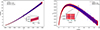 |
Fig. A.1. Comparison of DL(z) (left panel) and XH(z) (right panel) error estimates for BNSs observed during one-month and one-year DECIGO observations. The uncertainties of are evaluated with CNN. |
Appendix C: Systematical analysis
In this appendix we introduce several sources of systematics based on the one-year observation of DECIGO, which were considered in the above analysis. Firstly, the peculiar acceleration of each binary source could possibly act as an additional noise when measuring the redshift drift. However, the magnitude of peculiar acceleration expected in typical clusters and galaxies is much smaller than the measurement errors of Δtz due to detector noise (Amendola et al. 2008; Uzan et al. 2008). Secondly, the performance of DECIGO is evaluated on the Fisher information matrix method for the uncertainty assessment. Such statistics estimates the uncertainty of binary parameters θi via  (Cutler & Flanagan 1994). Our findings demonstrated the effectiveness of the machine learning method in accurately inferring the necessary variables and uncertainties. This result is consistent with the one in Sun et al. (2024). Thirdly, comparing the vg measurements on the ΛCDM cosmology from Planck 2018 results (Planck Collaboration VI 2020), we found that the systematics caused by different fiducial cosmologies are negligible. The fourth issue that needs clarification is the impact of degeneracies between mass and redshift. A recent review of the measurements from GWs of BNS (Landry & Read 2021), pulsars with radio timing, NS with high and low stellar mass companions using X-ray and optical observations (Alsing et al. 2018) showed that the mass distribution of neutron stars is very narrow (m = 1.27 ± 0.04 M⊙) (You et al. 2025). The impact of such small prior variance on the inverse Fisher matrix for DL(z) and XH(z) (and also other parameters) is of the order 𝒪(σℳBNS2). Therefore, introducing the prior σmNS ≈ 0.04 M⊙ in our calculations would not significantly affect the results regarding the final measurement of vg. Finally, modified gravity theories could possibly affect the estimation of BNS parameters and thus the determination accuracy of vg. The easiest modification is to add some scalar degrees of freedom to gravity (Brans & Dicke 1961) and one of the first models of this kind is the Brans-Dicke scalar-tensor theory of gravity. Such gravity theory will reduce to GR in the limit of ωBD → ∞ where ωBD is the Brans-Dicke parameter (Yagi & Tanaka 2010). Our analysis indicated that the inclusion of such modified gravity theory will result in systematic uncertainties in the extraction of vg. However, if we imposed the prior information of the source orientation, the constraint would become much stronger.
Finally, we emphasize that our analysis can be extended to the measurements of GW dispersion. Following Abbott et al. (2017c), we consider the following modified dispersion relation of E2 = p2c2 + Apαcα, α ≥ 0, where E and p denote the energy and momentum of gravitational radiation. A change in the amplitude of dispersion relation A could modify the GW group velocity as vg/c = 1 + (α − 1)AEα − 2/2 (Yunes et al. 2016). By introducing the evolution of GW phase in the effective-precession waveform model (Mirshekari et al. 2012), three BBH events (GW170104, GW150914 and GW151226) provided the credible upper bounds of dispersion parameter |A| as 10−19 PeV2 − α (Abbott et al. 2017c). However, this was achieved using only the high-frequency part of the GW signal. For several modified theories of gravity with various values of α, i.e. doubly special relativity (α = 3; Amelino-Camelia 2002), and extra-dimensional theory (α = 4; Sefiedgar et al. 2011), |A| is expected to be determined at the level of 10−5 TeV2 − α, through one-year observation of BNS events. In this aspect, multi-frequency studies involving DECIGO can effectively differentiate between GR and modified gravity theories, which strengthens its probative power to inspire new observing programs in the moderate future.
All Figures
|
Fig. 1. Measurements of the speed of GWs based on a one-month (upper panel) and a one-year (lower panel) observation of BNS events by DECIGO. The scale of departure from the GR δvg(flow)/c0 is assumed to be 10−4 and 10−5, respectively. |
| In the text | |
|
Fig. 2. Posterior distributions of vg determined by different techniques. DECIGO data under observing strategies I (one-month) and II (one-year) are compared with two other methods: a direct method based on transit time across a separated network of detectors, and an indirect method using the time delay of GW170817. Two strategies were considered: LIGO O2 – data from O2 of Advanced LIGO-Virgo – and LIGO O2 fixed – where the sky localization of the BNS source is fixed. Note that LIGO O2 and GW170817 only provide constraints on vg/c, and at low redshifts, we take c = c0 in this figure. |
| In the text | |
|
Fig. A.1. Comparison of DL(z) (left panel) and XH(z) (right panel) error estimates for BNSs observed during one-month and one-year DECIGO observations. The uncertainties of are evaluated with CNN. |
| In the text | |
Current usage metrics show cumulative count of Article Views (full-text article views including HTML views, PDF and ePub downloads, according to the available data) and Abstracts Views on Vision4Press platform.
Data correspond to usage on the plateform after 2015. The current usage metrics is available 48-96 hours after online publication and is updated daily on week days.
Initial download of the metrics may take a while.