| Issue |
A&A
Volume 704, December 2025
|
|
|---|---|---|
| Article Number | A194 | |
| Number of page(s) | 11 | |
| Section | Planets, planetary systems, and small bodies | |
| DOI | https://doi.org/10.1051/0004-6361/202554335 | |
| Published online | 16 December 2025 | |
HARPS-N reveals a well-aligned orbit for the highly eccentric warm Jupiter TOI-4127 b
1
Department of Physics and Astronomy, The University of New Mexico,
Albuquerque,
NM
87106,
USA
2
Instituto de Astrofísica de Canarias (IAC),
38200
La Laguna,
Tenerife,
Spain
3
Departamento de Astrofísica, Universidad de La Laguna (ULL),
38206
La Laguna,
Tenerife,
Spain
4
Center for Computational Astrophysics, Flatiron Institute,
162 Fifth Avenue,
New York,
NY
10010,
USA
5
Department of Astronomy, University of Illinois at Urbana-Champaign,
Urbana,
IL
61801,
USA
6
INAF – Osservatorio Astrofisico di Torino,
Via Osservatorio 20,
10025
Pino Torinese,
Italy
★ Corresponding author: This email address is being protected from spambots. You need JavaScript enabled to view it.
Received:
28
February
2025
Accepted:
1
October
2025
Abstract
Context. While many hot Jupiter systems have an obliquity measurement, the data on warm Jupiter systems are lacking. The longer orbital periods and transit durations of warm Jupiters make it more difficult to measure the obliquities of their host stars. However, the longer periods also mean that any misalignments persist due to the longer tidal realignment timescales. As a result, measuring these obliquities is necessary to improve our understanding how these types of planets form and how their formation and evolution differ from the processes characterizing hot Jupiters.
Aims. Here, we report the measurement of the Rossiter-McLaughlin effect for the TOI-4127 system using the HARPS-N spectrograph.
Methods. We modeled the system using our new HARPS-N radial velocity measurements, along with archival TESS photometry and NEID and SOPHIE radial velocities.
Results. We find that the host star is well-aligned with the highly eccentric (e=0.75) warm Jupiter TOI-4127 b, with a sky-projected obliquity of λ = 4−16+17∘. This makes TOI-4127 one of the most eccentric well-aligned systems to date and one of the longest periods for a system with a measured obliquity.
Conclusions. The origin of its highly eccentric, yet well-aligned orbit remains a mystery, however, and we investigate possible scenarios that could explain it. While typical in situ formation and disk migration scenarios cannot explain this system, certain scenarios involving resonant interactions between the planet and protoplanetary disk could. Similarly, specific cases of planet-planet scattering or Kozai-Lidov oscillations can result in a highly-eccentric and well-aligned orbit. Coplanar high-eccentricity migration could also explain this system. However, scenarios involvng this mechanism or Kozai-Lidov oscillations would require an additional planet in the system, which has not yet been detected in this case.
Key words: planets and satellites: gaseous planets / planets and satellites: individual: TOI-4127 b
© The Authors 2025
 Open Access article, published by EDP Sciences, under the terms of the Creative Commons Attribution License (https://creativecommons.org/licenses/by/4.0), which permits unrestricted use, distribution, and reproduction in any medium, provided the original work is properly cited.
This article is published in open access under the Subscribe to Open model. This email address is being protected from spambots. You need JavaScript enabled to view it. to support open access publication.
1 Introduction
Despite their intrinsic rarity, close-in giant planets make up a significant portion of the over 6000 exoplanets discovered to date. These close-in giants can be divided into two populations, known as hot and warm Jupiters, which have significant differences in system and orbital architectures. Warm Jupiters are located far enough from their host stars that tidal dissipation is not efficient at circularizing or realigning their orbits, with pericenter distances of a(1-e) ≿ 0.1 AU. For a warm Jupiter in a circular orbit around a Sun-like star, this corresponds to an orbital period of ∼10 days. While determining the eccentricities of these planets comes naturally when we are simultaneously measuring the masses from RVs, measuring the spin-orbit alignment of these systems is more challenging. The long orbital periods and transit durations of warm Jupiters results in fewer opportunities to measure the stellar obliquity through the Rossiter-McLaughlin (RM) effect (McLaughlin 1924; Rossiter 1924). The RM effect can only measure the sky-projected stellar obliquity, λ, since obtaining the true 3D obliquity, ψ, requires knowing the stellar inclination. However, measuring the inclination of a host star requires asteroseismology or a precise rotation period, which are not always readily obtainable.
Although many hot Jupiter host stars have reported obliquities, very few warm Jupiter host stars have this information available (Albrecht et al. 2022). Hot Jupiter systems show a wide range of obliquities (Dong & Foreman-Mackey 2023; Siegel et al. 2023), especially hot Jupiters around stars above the Kraft break (Kraft 1967), which show a much greater misalignment than those orbiting cooler stars (Winn et al. 2010). On the other hand, the few warm Jupiter systems with obliquity measurements generally show well-aligned systems regardless of host stars (Rice et al. 2022; Wang et al. 2024). Unlike the case of many well-aligned hot Jupiters, tidal realignment is not sufficient to explain well-aligned warm Jupiters, since the realignment timescales exceed the lifetimes of the host stars even in the case of cool dwarfs (Albrecht et al. 2012). In this way, the impact of a system’s dynamical history is preserved. Of the warm Jupiter systems with significantly misaligned orbits, most contain a stellar companion (Espinoza-Retamal et al. 2023).
In addition to having more generally well-aligned orbits, warm Jupiter systems are also more likely to host nearby additional planets than hot Jupiter systems (Huang et al. 2016; Wu et al. 2023), indicating that different formation and evolution pathways are responsible for the two types of systems. Warm Jupiter systems are thought to largely be the product of in situ formation (e.g., Boley et al. 2016) or disk migration (e.g., Baruteau et al. 2014), both of which allow for nearby planets and also produce well-aligned orbits. On the other hand, hot Jupiter systems are likely the result of high-eccentricity migration mechanisms (Petrovich & Tremaine 2016), processes that result in isolated planets often in misaligned orbits. Such mechanisms include Kozai-Lidov oscillations (e.g., Fabrycky & Tremaine 2007) and planet-planet scattering (e.g., Petrovich et al. 2014), although the latter mechanism can occasionally result in well-aligned, short-period giant planets (Marzari & Weidenschilling 2002). As the orbits of migrating hot Jupiters shrink and circularize, there is a time when they end up having orbital periods that are the same as those of warm Jupiters. If the migration mechanism is not efficient, they can end up “stuck” at these longer orbital periods in highly eccentric orbits. As such, it is possible that some of the warm Jupiters observed at present are actually either hot Jupiters migrating to their final orbit or “failed” hot Jupiters. If some of the more eccentric warm Jupiters are indeed migrating or failed hot Jupiters, then they should likely have misaligned orbits. This is thought to be the case for extremely eccentric and misaligned warm Jupiters, such as HD 80606 b (Pont et al. 2009) and the recently discovered TIC 241249530 b (Gupta et al. 2024). However, these highly eccentric warm Jupiters are not always misaligned, as is the case with TOI-3362 b (Espinoza-Retamal et al. 2023).
Here, we present the RM effect measurement for the TOI-4127 system. TOI-4127 b is a highly eccentric (e=0.75) warm Jupiter orbiting an F star (R⋆ = 1.29 R⊙, Teff = 6096 K) on a 56.4 day orbit (Gupta et al. 2023). Using new HARPS-N radial velocity measurements alongside archival TESS photometry and NEID and SOPHIE spectroscopy, we obtained a sky-projected obliquity of  . This makes TOI-4127 the newest addition to the small, but growing sample of highly eccentric, yet well-aligned warm Jupiter systems. In Sect. 2, we describe the newly obtained HARPS-N spectroscopy and archival TESS photometry and NEID and SOPHIE spectroscopy used to model the system. We describe the analysis we carried out to characterize the orbit and obtain system parameters in Sect. 3. We discuss possible formation and evolution scenarios and the system’s place in the larger sample of warm Jupiter systems in Sect. 4. We summarize our results in Sect. 5.
2 Observations
2.1 HARPS-N spectroscopy
We observed a transit of TOI-4127 b on 15 March 2024 using the High Accuracy Radial velocity Planet Searcher North (HARPS-N) spectrograph at the Telescopio Nazionale Galileo (TNG) at the Roque de los Muchachos Observatory, which observes at a wavelength range of 378-691 nm with a resolution R=115 000 (Cosentino et al. 2012). We obtained 15 1200-second observations spanning 4.8 hours, covering a 1.7 hours of pre-transit baseline and 3.1 hours of the transit. We also obtained one 1200-second pre-transit observation on 24 November 2023 with HARPS-N before high humidity prevented the rest of the observations from being taken. The air masses ranged from 1.38 to 1.8, while the signal-to-noise ratio ranged from 26.8 to 37.1. We obtained a median RV uncertainty of 6.88 m s−1 across the 16 observations.
The HARPS-N spectra time series were reduced using the offline data reduction software (DRS), which also computes radial velocities based on the cross-correlation function (CCF) method (Pepe et al. 2002). In this method, the spectra are cross-correlated with a binary mask created from a template spectrum matching the target star’s type. For our analysis, we chose the G2 mask, as it was the closest available match to the stellar type of TOI-4127. We reprocessed the data using the Yabi web application Hunter et al. 2012, accessible at the IA2 Data Centre1. The RVs are presented in Table A.1.
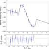 |
Fig. 1 Phase-folded HARPS-N radial velocities and best-fit model. |
2.2 Archival observations
We used the TESS (Ricker et al. 2015) Presearch Data Conditioning Simple Aperture Photometry (PDCSAP; Smith et al. 2012; Stumpe et al. 2012, 2014) photometry used by Gupta et al. (2023). This consists of two sectors (20 and 26) of 30-minute cadence full-frame image data and three sectors (40, 47, and 53) of 2-minute cadence postage stamps. TOI-4127 b transited in four of the five sectors; however, the transit in sector 47 was contaminated by scattered light and not included in the analysis (Fig. 2). Although the target was re-observed within a 2-minute cadence in sectors 73 and 74, the transit in sector 74 was also contaminated by scattered light and, thus, also excluded from the analysis. The three uncontaminated transits do not show any evidence for significant transit timing variations (Gupta et al. 2023) and are shown alongside the best-fit model in Fig. 3.
We also included the 30 radial velocity measurements used by Gupta et al. (2023) in our analysis: 11 from the NEID spectrograph on the WIYN 3.5 m telescope at Kitt Peak National Observatory (Schwab et al. 2016) and 19 from the SOPHIE spectrograph on the 1.93 m telescope at the Observatoire de Haute-Provence, France (Perruchot et al. 2008). The data and best-fit model are shown in Fig. 4. We used archival high-resolution imaging from NESSI on the WIYN 3.5 m telescope to help constrain possible unseen stellar companions, as described in Sect. 4.2.
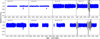 |
Fig. 2 TESS PDCSAP 30 minute (sectors 20 and 26) and 2-minute (sectors 40, 47, 53, 60, 73, and 74) cadence photometry of TOI-4127. Gray points denote low-quality simple aperture photometry (SAP) photometry not included in the analysis, while the magenta triangles denote the transit times of the two transits contaminated by scattered light. |
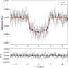 |
Fig. 3 Phase-folded TESS light curve zoomed in on the transit. The black and gray points denote 30-minute and 2-minute cadence data, respectively. The best-fit model is shown in red. |
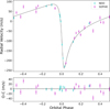 |
Fig. 4 Phase-folded NEID (cyan) and SOPHIE (magenta) radial velocities, with the best-fit model shown in black. |
3 Analysis
3.1 Stellar parameters
We adopted the stellar parameters from Gupta et al. (2023), which are shown in Table 1. The spectroscopic parameters were derived by using SpecMatch-Emp (Yee et al. 2017) to compare the NEID spectra to reference spectra, while the physical parameters were derived through SED analysis and mass-radius relations. We attempted to determine the stellar inclination by measuring the rotation period of the host star using a generalized Lomb-Scargle (GLS) periodogram on the TESS data. While some individual sectors of PDCSAP data showed statistically significant peaks, the locations of the peaks varied sector by sector and were nonexistent in the SAP data as well as full frame image data from the Quick-Look Pipeline (QLP; Huang et al. 2020a,b). As such, we were unable to obtain a rotation period or, consequently, the stellar inclination; there, we were not able to obtain the true 3D obliquity.
3.2 Joint photometric-spectroscopic analysis
We performed a fitting for the system parameters using a modified version of the allesfitter package (Günther & Daylan 2021, 2019) and carrying out a joint analysis of the TESS photometry and NEID, SOPHIE, and HARPS-N radial velocities. The original version of allesfitter employs the ellc package (Maxted 2016) to model the light curve and RVs. ellc uses the formulation from Ohta et al. (2005) to model the RM effect, which does not include microturbulence or macroturbulence. The modified version we used was developed to include these parameters (Wang et al. 2024), which makes use of the formulation from Hirano et al. (2011) to model the RM effect through the tracit package (Hjorth et al. 2021; Knudstrup & Albrecht 2022). The light curve and out-of-transit RVs were modeled using the PyTransit (Parviainen 2015) and RadVel (Fulton et al. 2018) packages, respectively. We used a nested sampling algorithm consisting of 500 live points to explore the parameter space and determine the best-fit values for the parameters listed in Table B.1, using uniform priors for all except two parameters. We used the empirical relations from Doyle et al. (2014) and Bruntt et al. (2010) to determine the values of the macroturbulence and microturbulence, respectively. We then used normal priors centered on those values for the two parameters, with σ = 1 km s−1.
The values and uncertainties of the fitted and derived parameters listed in Table B.1 are defined as the median values and 68% confidence intervals of the posterior distributions, respectively. The best-fit phase folded transit model is shown alongside the TESS data in Fig. 3. The best-fit RV model and NEID and SOPHIE data are shown in Fig. 4, while the best-fit RM model and HARPS-N data are shown in Fig. 1. The corner plots for the modeled and derived parameters are shown in Figs. C.1 and C.2.
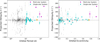 |
Fig. 5 Left panel: projected obliquities of warm Jupiter systems (10 d < P < 200 d and Rp > 6 R⊕) as a function of orbital period. Warm Jupiters in single-star and multi-star systems are shown in cyan and magenta, respectively. The single-star TOI-4127 system is shown in gold. All other systems with measured obliquities are shown in black. Right panel: projected obliquities as a function of orbital eccentricity. System parameters were obtained from TEPCat (Southworth 2011). |
System information.
4 Discussion
The joint analysis of the TESS, NEID, SOPHIE, and HARPSN data shows that TOI-4127 b is well-aligned with its host star, with a projected obliquity of  . This makes it one of the longest-period and most eccentric planets with an available obliquity measurement and the longest-period warm Jupiter on a well-aligned orbit (Fig. 5). It adds to the growing sample of highly eccentric yet well-aligned warm Jupiters that reside in single-star systems compared to the misaligned warm Jupiters in multi-star systems. Of the five most eccentric single-star warm Jupiter systems, three contain warm Jupiters with masses greater than two Jupiter masses, including TOI-4127. However, the other two do not have reported mass measurements and, thus, more measurements are needed to determine the role that planet mass plays in the trends observed. Smaller planets may also follow a similar trend of high eccentricity and low obliquity, as shown by the highly eccentric and possibly aligned sub-Saturn Kepler-1656 b (Rubenzahl et al. 2024), although a much larger sample is needed.
Despite a high orbital eccentricity of 0.75 ± 0.01, TOI-4127 b is not a hot Jupiter progenitor undergoing high-eccentricity migration unless it is undergoing eccentricity oscillations with intervals of even higher eccentricity. Gupta et al. (2023) found that the timescale for this planet to migrate and become a hot Jupiter is on the order of 780 Gyr given its current eccentricity. The question of how this planet could be so eccentric, yet also well-aligned (based on a number of commonly invoked formation and migration mechanisms) remains an open question. Similarly eccentric warm Jupiters such as TOI-3362 b and HD 17156 b are closer in to their host stars and, unlike TOI-4127 b, they reside in the region of parameter space where high-eccentricity tidal migration can take place (Fig. 6). Further out warm Jupiters like HD 80606 b and TIC 241249530 b are more eccentric than TOI-4127 b and reside in known multi-star systems unlike TOI-4127 b.
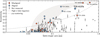 |
Fig. 6 Eccentricity vs. semimajor axis for all confirmed transiting planets between 6–20 Earth radii. Colored circles are planets with measured spin-orbit angles. Blue circles are defined as aligned with spin-orbit angles of less than 30 degrees, and red circles are defined as misaligned with spin-orbit angles greater than 30 degrees. The gray region illustrates planets that are likely undergoing high-eccentricity tidal migration. The upper and lower limits of the track are set by the Roche limit and the tidal circularization timescale (Dong et al. 2021). The dotted-dashed line presents the theoretical upper limit of eccentricities as a result of planet-planet scattering, assuming a planet with a mass of 0.5 MJup and a radius of 2 RJup, for illustrative purposes (Petrovich et al. 2014). The data were compiled from the NASA Exoplanet Archive as of October 30, 2024 (Christiansen et al. 2025). Stellar obliquity measurements were obtained from Knudstrup et al. (2024), in particular, Table B2, with recent updates. |
4.1 Formation pathways
The typical mechanisms invoked for in situ formation and disk migration are not sufficient explain the system. These mechanisms are able to explain the low obliquity of TOI-4127, but not the planet’s high eccentricity. Some disk migration mechanisms (e.g., planetary migration in a disk cavity) can excite the eccentricity of a resulting planet, but only up to a value of ~0.4 (Debras et al. 2021), which is far below TOI-4127 b’s eccentricity of 0.75. However, more recent dynamical simulations have shown that it is possible for a massive planet in a cavity to obtain high eccentricities solely through resonant interactions with the protoplanetary disk (Romanova et al. 2023, 2024). These interactions excite the eccentricity without misaligning with the orbit and the evolution timescales shorten significantly for more massive planets. The three most eccentric well-aligned warm Jupiters (HD 17156 b, TOI-3362 b, and TOI-4127 b) have masses greater than 2 MJup and could point toward this mechanism being responsible for this phenomenon. However, a larger sample of well-characterized systems is needed to draw any meaningful conclusions. Using the NASA Exoplanet Archive (Christiansen et al. 2025), we find that there are eight highly-eccentric (e > 0.5) giant planets (Rp > 6 R⊕) that are amenable for RM observations aimed at measuring their obliquities, meaning that they orbit stars brighter than V=12.5. These eight planets are TOI-2134 c, TOI-6883 b, TOI-5110 b, TOI-4582 b, TOI-2589 b, TOI-2179 b, Kepler-432 b, and TOI-2338 b. Five planets orbit main sequence FGK stars, while the other three orbit evolved stars (two sub-giants and one red giant). They range in masses from 0.13 to 5.98 MJup and in orbital periods from 15 to 111 days. We used Eq. (1) from Triaud (2018) to estimate the semi-amplitudes of the RM effect, finding that they range from 3 to 24 m s−1. While the lower amplitude signals will be challenging, detecting the signals is feasible with current instruments.
Kozai-Lidov oscillations and planet-planet scattering are often cited as the mechanisms responsible for hot Jupiters and their progenitors, failed or otherwise. However, these mechanisms typically result in highly-eccentric, misaligned systems. Kozai-Lidov oscillations might be able to explain this system when we happen to be observing it during a period of low obliquity. In this case, it would be indicative of an additional undetected planetary or stellar companion in the system. Similarly, planet-planet scattering can occasionally result in highly-eccentric well-aligned systems, as theorized for HD 17156 b in prior studies (Barbieri et al. 2009). If, in fact, there are no additional massive companions in the system, then this scenario would explain the orbit.
Another plausible explanation is that this system is the result of coplanar high-eccentricity migration (CHEM; Petrovich 2015). This mechanism is thought to be responsible for the well-aligned orbit of the similarly highly-eccentric warm Jupiter TOI-3362 b (Espinoza-Retamal et al. 2023). However, TOI-4127 b’s larger orbit means its eccentricity is slightly lower than what would be expected for a planet undergoing this process. This can be resolved, however, if it is still coupled to the perturber and undergoing eccentricity oscillations. Both this mechanism and some Kozai-Lidov oscillations scenarios require a second giant planet in the system that has yet to be detected. Gupta et al. (2023) synthesized and examined a sample of perturbers capable of inducing eccentricity oscillations and found that the existing RV data ought to have found many of such potential planets. Lower mass planets would have avoided detection thus far, as would the longest period planets (∼10 000 d). This sample overlaps significantly with the sample of planets capable of inducing coplanar high-eccentricity migration. A larger fraction of this sample has been ruled out; however there are many scenarios where a planet capable of inducing CHEM would not have been detected.
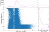 |
Fig. 7 Sample of stars consistent with current observations as determined by MOLUSC. The mass distribution peaks at low masses, while the semimajor axis distribution is bimodal. |
4.2 Potential stellar companions
If Kozai-Lidov oscillations are indeed responsible for the orbit of TOI-4127 b, then it could indicate that there is a stellar companion in the system, as is the case with HD 80606 b and TIC 241249530 b. While current observations have not led to the detection of a stellar companion, these observations have not probed all the possible parameter space. While radial velocity measurements have ruled out short-period stellar companions and high-resolution imaging has ruled out bright, distant companions, neither approach is sufficient to rule out stellar companions at more intermediate separations. Furthermore, TOI-4127 has a renormalized unit weight error (RUWE) of 1.27 in Gaia DR3. While RUWE values above 1.4 have been considered indicative of unresolved binaries in DR2 (Lindegren et al. 2018), the threshold for EDR3 is lower, at 1.25 (Penoyre et al. 2022). Thus, TOI-4127’s relatively high RUWE could be the result of an unseen stellar companion, which, in turn, could turn out to be TOI-4127 b’s perturber. In order to quantify possible undetected stellar companions, we used the Multi-Observational Limits on Unseen Stellar Companions (MOLUSC; Wood et al. 2021) code to generate a sample of potential companions consistent with the combination of the high-resolution imaging, RV data, Gaia astrometry (in the form of the RUWE), and Gaia imaging. Of the one million stars we generated using MOLUSC, only ∼10% were consistent with the aforementioned data. The sample peaks at low masses, in part due to only faint, low-mass stars being allowed at large separations (Fig. 7). The semimajor axis is bimodal, with the strongest peak at 1000 AU. Further observations are needed to determine whether there is a stellar companion in this system.
5 Conclusion
We analyzed the RM effect for the highly eccentric (e=0.75) warm Jupiter system TOI-4127 and found that it is well-aligned, with a sky-projected obliquity of  . It adds to the growing list of long-period systems with measured obliquities and is one of the most eccentric systems with such a measurement. There are multiple mechanisms that could explain this highly-eccentric yet well-aligned system, including resonant interactions with the protoplanetary disk, ongoing Kozai-Lidov oscillations, coplanar high-eccentricity migration, and planet-planet scattering. Both Kozai-Lidov oscillations and coplanar high-eccentricity migration scenarios would require additional companions in the system that have yet to be detected. A distant massive planet or stellar companions would favor Kozai-Lidov oscillations and a closer-in massive planet would favor coplanar high-eccentricity migration, whereas a lack of any massive companions would favor a scattering event. Additional RV measurements and future astrometric measurements from upcoming Gaia data releases will be able to determine whether there are additional planets or a stellar companion in this system that could help explain the orbit of TOI-4127 b.
Acknowledgements
We thank the anonymous referee for their helpful comments, which have helped improve the paper. We thank Xian-Yu Wang for his assistance with the modified version of allesfitter. This research has made use of the NASA Exoplanet Archive, which is operated by the California Institute of Technology, under contract with the National Aeronautics and Space Administration under the Exoplanet Exploration Program. D.D. acknowledges support from the NASA Exoplanet Research Program grant 18-2XRP18_2-0136. The Flatiron Institute is a division of the Simons foundation.
Reference
- Albrecht, S., Winn, J. N., Johnson, J. A., et al. 2012, ApJ, 757, 18 [NASA ADS] [CrossRef] [Google Scholar]
- Albrecht, S. H., Dawson, R. I., & Winn, J. N. 2022, PASP, 134, 082001 [NASA ADS] [CrossRef] [Google Scholar]
- Barbieri, M., Alonso, R., Desidera, S., et al. 2009, A&A, 503, 601 [NASA ADS] [CrossRef] [EDP Sciences] [Google Scholar]
- Baruteau, C., Crida, A., Paardekooper, S. J., et al. 2014, in Protostars and Planets VI, eds. H. Beuther, R.S. Klessen, C.P. Dullemond, & T. Henning (Tucson: University of Arizona Press), 667 [Google Scholar]
- Boley, A. C., Granados Contreras, A. P., & Gladman, B. 2016, ApJ, 817, L17 [Google Scholar]
- Bruntt, H., Bedding, T. R., Quirion, P. O., et al. 2010, MNRAS, 405, 1907 [Google Scholar]
- Christiansen, J. L., McElroy, D. L., Harbut, M., et al. 2025, Planet. Sci. J., 6, 186 [Google Scholar]
- Cosentino, R., Lovis, C., Pepe, F., et al. 2012, SPIE Conf. Ser., 8446, 84461V [Google Scholar]
- Cutri, R. M., Skrutskie, M. F., van Dyk, S., et al. 2003, VizieR Online Data Catalog: II/246 [Google Scholar]
- Debras, F., Baruteau, C., & Donati, J.-F. 2021, MNRAS, 500, 1621 [Google Scholar]
- Dong, J., & Foreman-Mackey, D. 2023, AJ, 166, 112 [NASA ADS] [CrossRef] [Google Scholar]
- Dong, J., Huang, C. X., Zhou, G., et al. 2021, ApJ, 920, L16 [NASA ADS] [CrossRef] [Google Scholar]
- Doyle, A. P., Davies, G. R., Smalley, B., Chaplin, W. J., & Elsworth, Y. 2014, MNRAS, 444, 3592 [Google Scholar]
- Espinoza-Retamal, J. I., Brahm, R., Petrovich, C., et al. 2023, ApJ, 958, L20 [NASA ADS] [CrossRef] [Google Scholar]
- Fabrycky, D., & Tremaine, S. 2007, ApJ, 669, 1298 [NASA ADS] [CrossRef] [Google Scholar]
- Fulton, B. J., Petigura, E. A., Blunt, S., & Sinukoff, E. 2018, PASP, 130, 044504 [Google Scholar]
- Gaia Collaboration (Vallenari, A., et al.) 2023, A&A, 674, A1 [NASA ADS] [CrossRef] [EDP Sciences] [Google Scholar]
- Günther, M. N., & Daylan, T. 2019, Astrophysics Source Code Library [record ascl:1903.003] [Google Scholar]
- Günther, M. N., & Daylan, T. 2021, ApJS, 254, 13 [CrossRef] [Google Scholar]
- Gupta, A. F., Jackson, J. M., Hébrard, G., et al. 2023, AJ, 165, 234 [NASA ADS] [CrossRef] [Google Scholar]
- Gupta, A. F., Millholland, S. C., Im, H., et al. 2024, Nature, 632, 50 [NASA ADS] [CrossRef] [Google Scholar]
- Hirano, T., Suto, Y., Winn, J. N., et al. 2011, ApJ, 742, 69 [NASA ADS] [CrossRef] [Google Scholar]
- Hjorth, M., Albrecht, S., Hirano, T., et al. 2021, Proc. Natl. Acad. Sci., 118, e2017418118 [NASA ADS] [CrossRef] [Google Scholar]
- Huang, C., Wu, Y., & Triaud, A. H. M. J. 2016, ApJ, 825, 98 [NASA ADS] [CrossRef] [Google Scholar]
- Huang, C. X., Vanderburg, A., Pál, A., et al. 2020a, Res. Notes Am. Astron. Soc., 4, 204 [Google Scholar]
- Huang, C. X., Vanderburg, A., Pál, A., et al. 2020b, Res. Notes Am. Astron. Soc., 4, 206 [Google Scholar]
- Hunter, A. A., Macgregor, A. B., Szabo, T. O., Wellington, C. A., & Bellgard, M. I. 2012, Source Code Biol. Medicine, 7, 1 [CrossRef] [Google Scholar]
- Knudstrup, E., & Albrecht, S. H. 2022, A&A, 660, A99 [NASA ADS] [CrossRef] [EDP Sciences] [Google Scholar]
- Knudstrup, E., Albrecht, S. H., Winn, J. N., et al. 2024, A&A, 690, A379 [NASA ADS] [CrossRef] [EDP Sciences] [Google Scholar]
- Kraft, R. P. 1967, ApJ, 150, 551 [Google Scholar]
- Lindegren, L., Hernández, J., Bombrun, A., et al. 2018, A&A, 616, A2 [NASA ADS] [CrossRef] [EDP Sciences] [Google Scholar]
- Marzari, F., & Weidenschilling, S. J. 2002, Icarus, 156, 570 [Google Scholar]
- Maxted, P. F. L. 2016, A&A, 591, A111 [NASA ADS] [CrossRef] [EDP Sciences] [Google Scholar]
- McLaughlin, D. B. 1924, ApJ, 60, 22 [Google Scholar]
- Ohta, Y., Taruya, A., & Suto, Y. 2005, ApJ, 622, 1118 [Google Scholar]
- Parviainen, H. 2015, MNRAS, 450, 3233 [Google Scholar]
- Penoyre, Z., Belokurov, V., & Evans, N. W. 2022, MNRAS, 513, 5270 [Google Scholar]
- Pepe, F., Mayor, M., Galland, F., et al. 2002, A&A, 388, 632 [NASA ADS] [CrossRef] [EDP Sciences] [Google Scholar]
- Perruchot, S., Kohler, D., Bouchy, F., et al. 2008, SPIE Conf. Ser., 7014, 70140J [Google Scholar]
- Petrovich, C. 2015, ApJ, 805, 75 [NASA ADS] [CrossRef] [Google Scholar]
- Petrovich, C., & Tremaine, S. 2016, ApJ, 829, 132 [NASA ADS] [CrossRef] [Google Scholar]
- Petrovich, C., Tremaine, S., & Rafikov, R. 2014, ApJ, 786, 101 [NASA ADS] [CrossRef] [Google Scholar]
- Pont, F., Hébrard, G., Irwin, J. M., et al. 2009, A&A, 502, 695 [NASA ADS] [CrossRef] [EDP Sciences] [Google Scholar]
- Rice, M., Wang, S., Wang, X.-Y., et al. 2022, AJ, 164, 104 [NASA ADS] [CrossRef] [Google Scholar]
- Ricker, G. R., Winn, J. N., Vanderspek, R., et al. 2015, J. Astron. Telesc. Instrum. Syst., 1, 014003 [Google Scholar]
- Romanova, M. M., Koldoba, A. V., Ustyugova, G. V., Lai, D., & Lovelace, R. V. E. 2023, MNRAS, 523, 2832 [Google Scholar]
- Romanova, M. M., Koldoba, A. V., Ustyugova, G. V., Espaillat, C., & Lovelace, R. V. E. 2024, MNRAS, 532, 3509 [Google Scholar]
- Rossiter, R. A. 1924, ApJ, 60, 15 [Google Scholar]
- Rubenzahl, R. A., Howard, A. W., Halverson, S., et al. 2024, ApJ, 971, L40 [Google Scholar]
- Schwab, C., Rakich, A., Gong, Q., et al. 2016, SPIE Conf. Ser., 9908, 99087H [NASA ADS] [Google Scholar]
- Siegel, J. C., Winn, J. N., & Albrecht, S. H. 2023, ApJ, 950, L2 [NASA ADS] [CrossRef] [Google Scholar]
- Smith, J. C., Stumpe, M. C., Van Cleve, J. E., et al. 2012, PASP, 124, 1000 [Google Scholar]
- Southworth, J. 2011, MNRAS, 417, 2166 [Google Scholar]
- Stassun, K. G., Oelkers, R. J., Pepper, J., et al. 2018, AJ, 156, 102 [Google Scholar]
- Stumpe, M. C., Smith, J. C., Van Cleve, J. E., et al. 2012, PASP, 124, 985 [Google Scholar]
- Stumpe, M. C., Smith, J. C., Catanzarite, J. H., et al. 2014, PASP, 126, 100 [Google Scholar]
- Triaud, A. H. M. J. 2018, in Handbook of Exoplanets, eds. H.J. Deeg, & J.A. Belmonte (Berlin: Springer), 2 [Google Scholar]
- Wang, X.-Y., Rice, M., Wang, S., et al. 2024, ApJ, 973, L21 [Google Scholar]
- Winn, J. N., Fabrycky, D., Albrecht, S., & Johnson, J. A. 2010, ApJ, 718, L145 [Google Scholar]
- Wood, M. L., Mann, A. W., & Kraus, A. L. 2021, AJ, 162, 128 [NASA ADS] [CrossRef] [Google Scholar]
- Wu, D.-H., Rice, M., & Wang, S. 2023, AJ, 165, 171 [NASA ADS] [CrossRef] [Google Scholar]
- Yee, S. W., Petigura, E. A., & von Braun, K. 2017, ApJ, 836, 77 [Google Scholar]
Appendix A HARPS-N radial velocities
In this appendix, we present the values of the HARPS-N radial velocities with their uncertainties.
HARPS-N RVs.
Appendix B TOI-4127 b parameters
In this appendix we present the values of the fitted and derived system parameters.
Planetary parameters.
Appendix C allesfitter corner plots
In this appendix we show the corner plots from our allesfitter fit.
 |
Fig. C.1 Corner plots of modeled parameters obtained from allesfitter. |
 |
Fig. C.2 Corner plots of derived parameters obtained from allesfitter. |
All Tables
All Figures
|
Fig. 1 Phase-folded HARPS-N radial velocities and best-fit model. |
| In the text | |
|
Fig. 2 TESS PDCSAP 30 minute (sectors 20 and 26) and 2-minute (sectors 40, 47, 53, 60, 73, and 74) cadence photometry of TOI-4127. Gray points denote low-quality simple aperture photometry (SAP) photometry not included in the analysis, while the magenta triangles denote the transit times of the two transits contaminated by scattered light. |
| In the text | |
|
Fig. 3 Phase-folded TESS light curve zoomed in on the transit. The black and gray points denote 30-minute and 2-minute cadence data, respectively. The best-fit model is shown in red. |
| In the text | |
|
Fig. 4 Phase-folded NEID (cyan) and SOPHIE (magenta) radial velocities, with the best-fit model shown in black. |
| In the text | |
|
Fig. 5 Left panel: projected obliquities of warm Jupiter systems (10 d < P < 200 d and Rp > 6 R⊕) as a function of orbital period. Warm Jupiters in single-star and multi-star systems are shown in cyan and magenta, respectively. The single-star TOI-4127 system is shown in gold. All other systems with measured obliquities are shown in black. Right panel: projected obliquities as a function of orbital eccentricity. System parameters were obtained from TEPCat (Southworth 2011). |
| In the text | |
|
Fig. 6 Eccentricity vs. semimajor axis for all confirmed transiting planets between 6–20 Earth radii. Colored circles are planets with measured spin-orbit angles. Blue circles are defined as aligned with spin-orbit angles of less than 30 degrees, and red circles are defined as misaligned with spin-orbit angles greater than 30 degrees. The gray region illustrates planets that are likely undergoing high-eccentricity tidal migration. The upper and lower limits of the track are set by the Roche limit and the tidal circularization timescale (Dong et al. 2021). The dotted-dashed line presents the theoretical upper limit of eccentricities as a result of planet-planet scattering, assuming a planet with a mass of 0.5 MJup and a radius of 2 RJup, for illustrative purposes (Petrovich et al. 2014). The data were compiled from the NASA Exoplanet Archive as of October 30, 2024 (Christiansen et al. 2025). Stellar obliquity measurements were obtained from Knudstrup et al. (2024), in particular, Table B2, with recent updates. |
| In the text | |
|
Fig. 7 Sample of stars consistent with current observations as determined by MOLUSC. The mass distribution peaks at low masses, while the semimajor axis distribution is bimodal. |
| In the text | |
|
Fig. C.1 Corner plots of modeled parameters obtained from allesfitter. |
| In the text | |
|
Fig. C.2 Corner plots of derived parameters obtained from allesfitter. |
| In the text | |
Current usage metrics show cumulative count of Article Views (full-text article views including HTML views, PDF and ePub downloads, according to the available data) and Abstracts Views on Vision4Press platform.
Data correspond to usage on the plateform after 2015. The current usage metrics is available 48-96 hours after online publication and is updated daily on week days.
Initial download of the metrics may take a while.