| Issue |
A&A
Volume 704, December 2025
|
|
|---|---|---|
| Article Number | A87 | |
| Number of page(s) | 5 | |
| Section | Astrophysical processes | |
| DOI | https://doi.org/10.1051/0004-6361/202554834 | |
| Published online | 05 December 2025 | |
X-ray linear polarization prediction in black hole binaries and active galactic nuclei and measurements of it by IXPE
1
INAF-IAPS, Via Fosso Del Cavaliere 100, 00133 Rome, Italy
2
Lomonosov Moscow State University/Sternberg Astronomical Institute, Universitetsky Prospect 13, Moscow 119992, Russia
⋆ Corresponding authors: This email address is being protected from spambots. You need JavaScript enabled to view it.
; This email address is being protected from spambots. You need JavaScript enabled to view it.
; This email address is being protected from spambots. You need JavaScript enabled to view it.
Received:
28
March
2025
Accepted:
6
June
2025
Abstract
Context. We present a theoretical framework for the formation of X-ray linear polarization in a black hole (BH) source. The X-ray linear polarization originates from up-scatterings of initially soft photons within a hot, optically thick Compton cloud (CC) characterized by a flat geometry. We demonstrated that the degree of linear polarization is independent of the photon energy and follows a characteristic angular distribution determined by the optical depth, τ0. For τ0 > 5, the linear polarization follows the Chandrasekhar classical distribution. The IXPE observations of several BHs’ X-ray binaries and of one Seyfert-1 galaxy confirm our theoretical prediction regarding the values of the linear polarization, P.
Aims. The goal of this paper is to demonstrate that the main physical parameters of these Galactic and extragalactic sources can be derived without any free parameter using the polarization and X-ray spectral measurements. These polarization measurements demonstrate that the polarization degree, P, is almost independent of energy.
Methods. We estimated the CC optical depth, τ0, for all BHs observed by IXPE, using the plot of P versus μ = cos i, where i is an observer inclination with respect to the normal, and considering the values, P, for a given source. Using X-ray spectral analysis, we obtained the photon index, Γ, and, analytically determined the CC plasma temperature, kBTe.
Results. Different BHs – in particular, Cyg X–1, 4U 1630–47, LMC X–1, 4U 1957+115, Swift J1727.8–1613, GX 339–4, and the Seyfert-1 BH, NGC 4151 – exhibit polarization at the 1%–8% level nearly independently of energy. kBTe is in the range of 5–90 keV, with a smaller value in the high-soft state with respect to the low-hard state. Remarkably, a polarization vector parallel to the CC plane can be excluded solely based on spectral constraints, in agreement with the IXPE observations.
Conclusions. Using IXPE results on polarization and the inclination of the system, we estimated τ0. Using the photon index, Γ, and τ0, we derived the plasma temperature, kBTe, without any free parameters. We find a similarity between the physical parameter and the IXPE findings and we provide evidence suggesting that the CC exhibits a flat geometry.
Key words: black hole physics / polarization / instrumentation: polarimeters / methods: analytical
© The Authors 2025
 Open Access article, published by EDP Sciences, under the terms of the Creative Commons Attribution License (https://creativecommons.org/licenses/by/4.0), which permits unrestricted use, distribution, and reproduction in any medium, provided the original work is properly cited.
This article is published in open access under the Subscribe to Open model. This email address is being protected from spambots. You need JavaScript enabled to view it. to support open access publication.
1. Introduction
Black hole (BH) X-ray binaries (BHXBs) evolve from a low lunimosity with hard spectrum state (LHS) to a high luminosity with soft spectrum state (HSS). In these states, the corona, presumably, dominates the X-ray emission, particularly in the LHS and the intermediate state (IS) (Montanari et al. 2009). But the geometry of the corona is not known yet. The geometries of the corona considered up to now are: a sphere above a BH as a lamp-post (Wilkins & Fabian 2012), a Compton cloud (CC) as a flat (planer) atmosphere (Haardt & Matt 1993), and a quasi-spherical CC between an accretion disk (AD) and a central BH (Shaposhnikov & Titarchuk 2006).
We return to the problem of the X-ray spectral formation in compact objects, in particular for BHs, because of the quite exact measurements of the linear polarization (LP) for these objects (see e.g., Krawczynski et al. 2022; Steiner et al. 2024; Dovčiak et al. 2024; Marin et al. 2024). We remind the reader details of the old paper (hereafter ST85) by Sunyaev & Titarchuk (1985), who investigated analytically the X-ray spectral and LP formation, P, in the slab (plain) geometry for a wide range of the Thomson optical depth from 0.1 to more than 10. It is remarkable that, for an optical depth (half of the slab) larger than 10, they obtained a value of polarization that follows the classical Chandrasekhar distribution versus the inclination, i, which is the angle between the direction of observation and the normal to the slab (Chandrasekhar 1950). It is well known that the shape of the observed X-ray spectra agrees with the analytically derived Comptonization spectra Sunyaev & Titarchuk (1980), Titarchuk (1994), hereafter ST80 and T94, respectively. In this paper, it is important to remind the reader of the expected characteristics of the linear X-ray polarization produced in a flat CC. We interpret the X-ray data from several Galactic BHXBs and one active galactic nucleus (AGN) for which remarkable polarization measurements have been obtained.
Stellar and supermassive BHs have similar accretion processes. All these BHs show similar components in their spectra: a thermal component in the soft X-ray spectra, and a Comptonization component in the hard X-rays. The thermal component is likely generated within the AD, which is typically presented as a geometrically thin, optically thick structure, such as the Shakura-Sunyaev disk (see Shakura & Sunyaev 1973). The Comptonized component is formed in the CC, a region of hot plasma that up-scatters photons from the AD to higher energies via inverse Compton scattering, producing the hard X-ray emission observed in BHXBs and AGNs (see Titarchuk 1994).
In the HSS, the AD blackbody emission dominates in the emergent spectrum (see the X-ray spectral evolution in a BH XTE J1650–500, Montanari et al. 2009). Some authors can think that in the HSS a geometrically thin optically thick AD continues down to the innermost stable circular orbit (Saade et al. 2024), while in the LHS the AD is possibly truncated. A cartoon showing the different geometry of a BH in the HSS and the LHS is shown in Fig. 1 in ST85 and in Fig. 3 here.
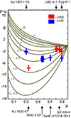 |
Fig. 1. Percentage of LP, P, as a function of μ = cos i, where i is the angle between the normal to the CC and a given direction (see ST85 and our Fig. 3). Red and blue boxes are drawn for the measured linear polarization degree in the 2–8 keV for the soft and hard states, correspondingly, for different BH sources (source names are indicated by arrows next to the corresponding μ). The vertical width of these boxes corresponds to the error bars of the IXPE measurements. |
Polarization provides a direct constraint on the geometry of the X-ray-emitting region that is not possible by timing and spectral measurements only. With this in mind, we applied this new independent way to derive relevant parameters of the accretion processes through the polarization data as demonstrated in ST85. For the first time ever, the Imaging X-ray Polarimetry Explorer (IXPE) (Weisskopf et al. 2022; Soffitta et al. 2021), a NASA-ASI mission with crucial INAF and INFN contributions that was launched on December 9, 2021, provides energy resolved X-ray polarization data in the 2–8 keV energy band for a large number of stellar BHs (Dovčiak et al. 2024) in their different states and for a few selected radio-quiet AGNs (Marin et al. 2024) .
In Sect. 2 we recall the polarization properties of the hard X-ray radiation produced within a planar CC around a BH. In Sect. 3 we use the polarization properties of BHs to derive the main parameters of these objects. In Sect. 4 we point out the importance of our results, and in Sect. 5 we draw the conclusions of our polarization study of the Galactic and extragalactic black holes (EBHs).
2. The polarization X-ray photons emerging from Compton clouds
We assume that a primary source of the soft photons is distributed over the CC slab with different configurations: in the center of the CC slab, a uniform distribution inside the cloud, or on the CC boundary. ST85 showed that the polarization properties of photons that undergo a number of scatterings, N ≫ τ02, much larger than the average, for a given optical depth of the CC slab, 2τ0 (see Fig. 1 in ST85), are independent of any of these distributions.
Up-scattering (Comptonization) of low-frequency (soft) photons of hν ≪ kBTe leads to energy gain up to photon energies, hν ≤ 3kBTe. A thermal, nonrelativistic (i.e., Maxwellian) electron distribution is considered (see ST80, ST85).
It is a remarkable result of ST85 that the polarization of X-ray photons should be independent of the photon energy, which is essentially confirmed by the IXPE observations. Solving the integro-differential equation of the transport of the polarized radiation, ST85 used the method of consecutive approximations. For k ≫ τ0 the polarization of photons after these k scatterings is independent of k (see ST85). When kBTe < 70 keV and the Thomson approximation is valid, the result of the ST85 calculations is correct (Pozdnyakov et al. 1983).
We introduce a two-component vector,  , denoting the radiation intensities related to the electric field oscillations in the plane defined by the disk axis and by direction of photon propagation (plane called meridional) and in the plane perpendicular, to it, respectively. Changes in Il and Ir in the CC plane have been calculated by the following transport equations (Chandrasekhar 1950):
 (1)
(1)
where dτ = −σTNedz, μ = cos i, and

is the scattering matrix. The vector  notes the distribution of primary sources. The boundary condition of the problem is
 (2)
(2)
for any 0 ≤ μ ≤ 1.
The degree of polarization is defined as
 (3)
(3)
and the intensity is a sum, I(0, μ) = Ir(0, μ)+Il(0, μ).
We should find the photon distribution that undergoes k scatterings. One should also determine the distribution of photons that are not scattered in the medium; namely,
![Mathematical equation: $$ \begin{aligned} {\bar{{I}} (\tau , \mu ) = \int _\tau ^{2\tau _0} \exp [{ -(\tau ^\prime -2\tau _0)/\mu )}]\bar{F}(\tau ^\prime })\mathrm{d}\tau ^{\prime }/\mu ,\end{aligned} $$](/articles/aa/full_html/2025/12/aa54834-25/aa54834-25-eq7.gif) (4)
(4)
for any initial photon distribution,  .
.
When the intensities of the first and next iterations are calculated one can proceed with the intensity of photons that undergo k scatterings:
 (5)
(5)
The solution of the k iteration depends on its solution for (k − 1) one (see also ST85).
In Table 1 of ST85, the authors showed that the polarization degree and angle distribution of k-scattered photons are independent of the primary source distribution if k ≫ τ0. To illustrate this statement, the authors made their calculations for τ0 = 2 and the iteration number N ≥ 20. The calculation results for k ≫ τ0 are independent of k and demonstrate that these results can be applied to the polarization of the Comptonized photons (see more details in ST85, Appendix A2). It is worth emphasizing that for large optical depths (τ ≫ 5) X-ray polarization converges on the classical solution by Sobolev (1949) and Chandrasekhar (1950). The change in the polarization sign for τ < 4 (see Fig. 1 and ST85) can be explained by a simple example of the optically thin CC (see Sect. 5.3 in ST85).
BHXRBs and AGN parameters including the best-fit photon index, α, the derived optical thickness, τ0, and the CC temperature, kBTe.
The appropriate radiative transfer equation, Eq. (1), can be rewritten in the operator form (see also Sect. A2 in ST85). The system of equations of the polarized radiation, Eq. (1), can be rewritten as
 (6)
(6)
where L is the polarization integral operator. One can check that the operator, L, meets all the conditions of the Hilbert-Schmidt theorem (see ST85). Thus, L has an eigenvalue,  , and ortho-normalized eigen functions, φi and pi → 0, while i → ∞. A vector function,
  , can be expanded in a generalized Fourier series:
 (7)
(7)
Solving Eq. (6) by the method of successive approximations, we find that the term  , related to the photons, underwent k scatterings:
 (8)
(8)
Because of the sequence of pi decreasing with k, we find that
 (9)
(9)
This mathematical result is illustrated by Table 2 of ST85 for k ≫ τ02.
3. Determination of the main parameters of the Compton cloud
Sunyaev & Titarchuk (ST80; see also ST85) solved the problem of X-ray spectral formation in the bounded medium. In particular, for the slab geometry they derived a formula for the spectral index, α (and Γ = α + 1):
 (10)
(10)
where γ = mec2β/kBTe, β = π2/[12(τ0 + 2/3)2], α = Γ − 1, and τ0 is the optical depth of one half of the slab.
Using these formulae one can find the electron temperature, kBTe, as a function of α and β:
 (11)
(11)
ST85 calculated the transfer of the polarized radiation using the iteration method. The number of iterations should be much more than the average number of scatterings in a given flat CC. As a result they made a plot of the LP of the Comptonized photons) as a function of μ = cos i, where i is the inclination of the system for different Thomson optical depths of τ0. ST85 calculated the LP for τ0 from 0.1 to 10, and for τ0 > 10 they found that the LP follows the well-known Chandrasekhar distribution (see Fig. 1).
For quite a few BHs, the LP, P, was measured. For example, for Cyg X-1 using IXPE data, (Steiner et al. 2024) showed that in the soft (HSS) and hard (LHS) states of the source, respectively, Ps ∼ (2 ± 0.5)% and Ph ∼ (3.5 ± 0.5)% are almost independent of the photon energy. The measured photon indices are ΓHSS = 2.5, ΓLHS = 1.4, and kBTe = 9 keV, and 90 keV, respectively (see Fig. 2 and Table 1).
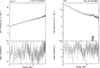 |
Fig. 2. IXPE spectra of Cyg X-1 for which X-ray polarization is detected during the LHS and HSS. The photon index is Γ = 1.4, Eline = 6.5 keV, and χred2 = 158/149; see left panel (ID = 01002901). For the HSS spectrum, these parameters are Γ = 2.4, Eline = 6.4 keV, and χred2 = 151/149; see right panel (ID=02008601). The best-fit model consists of const*tbabs*(comptb + Gaussian). |
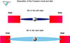 |
Fig. 3. Geometry of the CC. Using the polarimetric measurement, we assume that the planer CC is present. The CC is smaller and thicker for the soft state (dark blue) than that for the hard state (light blue). |
For the HSS of 4U 1630-47, (Rodriguez Cavero et al. 2023) found that Γ ∼ 2.6 − 2.9. The inclination, i, is in the range of 60 − 75° (see Kuulkers 1998), and using the plot of the LP versus μ (see Fig. 1) we find that τ0 is around 1.7 and kBTe ≈ 10 keV (see Eqs. (10) and (11) and Table 1]).
It is worth noting the trend of P, which ranges from 6−12% in the 2–8 keV energy band, as in Table 1 (Ratheesh et al. 2024). On the other hand, the photon indices, Γ, in these measurements vary from 2.6 to 4.5 (see Ratheesh et al. 2024 and also Rodriguez Cavero et al. 2023). This indicates that the polarization detections were made while the source underwent significant spectral state changes. It is important to emphasize that the quasi-constancy of P with energy can only be ensured if the P value is determined within the same spectral state.
For the BHXRB 4U 1957+115, (Marra et al. 2024, hereafter M24) obtained Ph = (1.9 ± 0.6)%, which is observed in the HSS. Knowing the inclination, i ∼ 72°, and using the LP versus μ plot, we find that τ0 ∼ 2.5 for 4U 1957+115 (Γ is about 2, see our Table 1). This is consistent with the result of M24, who found that Γ = 1.93 ± 0.21 (Table 1 in M24).
For LMC X–1 (Podgorný et al. 2023, hereafter P23) report an IXPE observation in the HSS using NICER, NuSTAR, and IXPE spectra (see their Fig. 3). The photon index, Γ ≈ 2.6, was obtained using the XSPEC NTHCOMP model. P23 assume that i is about 36°. Thus, using the P values and μ = cos36° ∼ 0.8, we find that the optical depth, τ0, is about 2.5.
For Swift J1727.8–1613 (Veledina et al. 2023), hereafter V23, report a significant polarization [P = (4.1 ± 0.2)%] that is almost independent of the photon energy (see Table 1 in V23). If we take into account that i is within the interval 30° −60° (Casares & Jonker 2014), then we obtain τ0 ∼ 1.5. V23 also report that Γ ∼ 1.8 is determined for a particular observation when the LP is about 4%. In this case the optical depth, τ0, is about 2.
For GX 339–4 (Mastroserio et al. 2025) published a significant (4σ) polarization degree, P = (1.3 ± 0.3)%, in the 3–8 keV band (where the spectrum is dominated by the corona) . We assume that the inclination in this source is 30° as a low limit (see Mastroserio et al. 2025, Table 3). Thus, we get a value of τ0 ≈ 3.
IXPE observed a select number of radio-quiet AGNs. One of the brightest Seyfert-1 galaxies, NGC 4151, shows a significant polarization, P = (4.5 ± 0.9)%, parallel to the radio emission. We obtain τ0 ≈ 2 using Fig. 1 and the inclination, i, within the range of 58.1° ±0.9° (Bentz et al. 2022).
4. Discussion
One can argue about the sign of the observed polarization degree (see Fig. 1). If one chooses positive values then one infers a value of τ0 > 5 for almost any value of μ = cos i. However, the derived value of τ0 > 5 contradicts the observed value of the index, Γ > 1.5 (α > 0.5), and the Comptonization parameter, Y ∼ (kBTe/mec2)(2τ0)2 ∝ α−1 (see Table 1). For these values of τ0 > 5, the Y parameter is higher than 2. In this case the emergent spectrum has a Wien shape (see e.g., Rybicki & Lightman 1979), which contradicts the X-ray observations.
We recall again here the definition of polarization described by ST85. Negative polarization of the observed radiation implies that the polarization vector lies within the meridional plane, which is the plane defined by the disk normal and the propagation direction of the outgoing photons. Indeed, the IXPE observations of BHXRBs and Seyfert-1 galaxies show that the polarization vector is consistently parallel to the disk axis for all of them (see, e.g., Krawczynski et al. 2022; Dovčiak et al. 2024; Marin et al. 2024). This confirms that the polarization vector resides within the meridional plane, explicitly ruling out polarization vectors oriented parallel to the disk plane.
The plane geometry is unexpected for the CCs. As we noted in the introduction, any type of CC geometry can be assumed: jets above the disk or a quasi-spherical CC around a BH. But there can only be strong LP if there is a strong asymmetry in the CC around a BH. It is natural that for the spherical CC around the central object (e.g., a NS) the polarization degree is close to zero (see e.g., Farinelli et al. 2024). If we choose negative values of polarization, P, then this leads to values of τ0 from 0.1 to 3 (see Figs. 5 and 8 in ST85 and Fig. 1 here).
Saade et al. (2024, hereafter S24) make a comparison of the X-ray polarimetric properties of stellar and supermassive BHs. In their Fig. 1, they present the polarization degree versus their inclination, i. The range of i for the Galactic BHs is almost determined, while EBHs have a very broad distribution (within approximately the 60° interval).
The PD values of these EBHs are typical of the ones calculated in ST85 and presented here in Fig. 1. It is not by chance that S24 noted that the polarization properties of these two types of sources are similar. It is easy to see that the range of the optical depth, τ0, in this case can be estimated within an interval of 1 − 1.5. If these EBHs are observed in the LHS then Γ < 2 and the electron temperature is kBTe ∼ 40 − 60 keV (see Table 1).
It is well known that the best-fit values of the optical depth, τ, and kBTe are around 2 and 60 keV, respectively, in the LHS and τ > 3, kBTe < 10 keV in the HSS (see Table 1 and e.g., ST85, T94).
5. Conclusions
A theoretical idea of the LP formation in a BH relies on the ST85 study. The linearly polarized X-ray radiation is the result of the multiple up-scattering of the initially X-ray soft photons (or UV ones in the AGN case) by the hot CC. Multiple scattering of the soft disk photons leads to the formation of the relatively hard emergent Comptonization spectrum. Furthermore, this specific spectrum is linearly polarized if the CC has a flat geometry. The polarization degree of these multiple up-scattered photons, P, should be independent of the photon energy.
ST85 made a plot of P as a function of μ = cos i, where i is inclination of the source. For different Thomson optical depths, τ0, of the flat CC, ST85 calculated the LP, P, for τ0 from 0.1 to 10 (see also their Figs. 5 and 8).
IXPE observed quite a few BHs and these observations have already been analyzed (see e.g., Dovčiak et al. 2024). Cyg X–1 data were studied by Krawczynski et al. (2022), Steiner et al. (2024), who established that in the soft and hard states Ps ∼ 2% and Ph ∼ 3.5%, respectively. Rodriguez Cavero et al. (2023) analyzed the data for 4U 1630–47 and found that Ph ∼ 7%. Marra et al. (2024) analyzed the data from a BH source, 4U 1957+115. They obtained Ph ∼ 2%.
The analysis of IXPE data for LMC X–1 was made by Podgorný et al. (2023) finding that P is about 1%, while for 4U 1630–47 Rodriguez Cavero et al. (2023) found P to be about 7%. In the case of Swift J1727.8–1613 (Veledina et al. 2023) reported that P ∼ 4%. For GX 339–4 an analysis of IXPE observations was made by Mastroserio et al. (2025) finding that P ∼ 1.3%. Finally for a bright Seyfert-1 galaxy (NGC 4151), Gianolli et al. (2024) found P ∼ 4.5%. For all these BHs, using the plot of P versus μ and values P for a given source, we estimated the CC optical depth, τ0, and using the results of the spectral analysis, we obtained the photon index, Γ, and the plasma temperature, kBTe, without any free parameters (see Table 1).
IXPE observed a polarization vector aligned to the disk axis. This is consistent with the negative polarization inferred in this work based on a spectral shape analysis. A similar pattern is observed in radio-quiet Seyfert 1 galaxies studied by IXPE (Marin et al. 2024), highlighting a remarkable similarity across BHs that spans an enormous range of BH masses (e.g., see Saade et al. 2024).
Acknowledgments
The Imaging X-ray Polarimetry Explorer (IXPE) is a joint US and Italian mission. The US contribution is supported by the National Aeronautics and Space Administration (NASA) and led and managed by its Marshall Space Flight Center (MSFC), with industry partner Ball Aerospace (now, BAE Systems). The Italian contribution is supported by the Italian Space Agency (Agenzia Spaziale Italiana, ASI) through contract ASI-OHBI-2022-13-I.0, agreements ASI-INAF-2022-19-HH.0 and ASI-INFN-2017.13-H0, and its Space Science Data Center (SSDC) with agreements ASI-INAF-2022-14-HH.0 and ASI-INFN 2021-43-HH.0, and by the Istituto Nazionale di Astrofisica (INAF) and the Istituto Nazionale di Fisica Nucleare (INFN) in Italy. This research used data products provided by the IXPE Team (MSFC, SSDC, INAF, and INFN) and distributed with additional software tools by the High-Energy Astrophysics Science Archive Research Center (HEASARC), at NASA Goddard Space Flight Center (GSFC). In addition, we acknowledge the fruitful discussion with the referee on the content of the presented paper.
References
- Bentz, M. C., Williams, P. R., & Treu, T. 2022, ApJ, 934, 168 [CrossRef] [Google Scholar]
- Casares, J., & Jonker, P. G. 2014, Space Sci. Rev., 183, 223 [NASA ADS] [CrossRef] [Google Scholar]
- Chandrasekhar, S. 1950, Radiative Transfer (Oxford: Clarendon Press) [Google Scholar]
- Dovčiak, M., Podgorný, J., Svoboda, J., et al. 2024, Galaxies, 12, 54 [CrossRef] [Google Scholar]
- Farinelli, R., Waghmare, A., Ducci, L., & Santangelo, A. 2024, A&A, 684, A62 [NASA ADS] [CrossRef] [EDP Sciences] [Google Scholar]
- Gianolli, V. E., Bianchi, S., Kammoun, E., et al. 2024, A&A, 691, A29 [NASA ADS] [CrossRef] [EDP Sciences] [Google Scholar]
- Haardt, F., & Matt, G. 1993, MNRAS, 261, 346 [NASA ADS] [CrossRef] [Google Scholar]
- Krawczynski, H., Muleri, F., Dovčiak, M., et al. 2022, Science, 378, 650 [NASA ADS] [CrossRef] [Google Scholar]
- Kuulkers, E. 1998, New Astron. Rev., 42, 613 [Google Scholar]
- Marin, F., Gianolli, V. E., Ingram, A., et al. 2024, Galaxies, 12, 35 [NASA ADS] [CrossRef] [Google Scholar]
- Marra, L., Brigitte, M., Rodriguez Cavero, N., et al. 2024, A&A, 684, A95 [NASA ADS] [CrossRef] [EDP Sciences] [Google Scholar]
- Mastroserio, G., De Marco, B., Baglio, M. C., et al. 2025, ApJ, 978, L19 [Google Scholar]
- Montanari, E., Titarchuk, L., & Frontera, F. 2009, ApJ, 692, 1597 [Google Scholar]
- Podgorný, J., Marra, L., Muleri, F., et al. 2023, MNRAS, 526, 5964 [CrossRef] [Google Scholar]
- Pozdnyakov, L. A., Sobol, I. M., & Syunyaev, R. A. 1983, Astrophys. Space Phys. Res., 2, 189 [Google Scholar]
- Ratheesh, A., Dovčiak, M., Krawczynski, H., et al. 2024, ApJ, 964, 77 [NASA ADS] [CrossRef] [Google Scholar]
- Rodriguez Cavero, N., Marra, L., Krawczynski, H., et al. 2023, ApJ, 958, L8 [NASA ADS] [CrossRef] [Google Scholar]
- Rybicki, G. B., & Lightman, A. P. 1979, Radiative Processes in Astrophysics (New York: Wiley-Interscience), 393 [Google Scholar]
- Saade, M. L., Kaaret, P., Liodakis, I., & Ehlert, S. R. 2024, ApJ, 974, 101 [Google Scholar]
- Shakura, N. I., & Sunyaev, R. A. 1973, A&A, 24, 337 [NASA ADS] [Google Scholar]
- Shaposhnikov, N., & Titarchuk, L. 2006, ApJ, 643, 1098 [NASA ADS] [CrossRef] [Google Scholar]
- Sobolev, V. V. 1949, Uchenye Zapisky Leningrad. Univ., Seria, Matem. Nauk, 18, N1163 [Google Scholar]
- Soffitta, P., Baldini, L., Bellazzini, R., et al. 2021, AJ, 162, 208 [CrossRef] [Google Scholar]
- Steiner, J. F., Nathan, E., Hu, K., et al. 2024, ApJ, 969, L30 [NASA ADS] [CrossRef] [Google Scholar]
- Sunyaev, R. A., & Titarchuk, L. G. 1980, A&A, 86, 121 [NASA ADS] [Google Scholar]
- Sunyaev, R. A., & Titarchuk, L. G. 1985, A&A, 143, 374 [NASA ADS] [Google Scholar]
- Titarchuk, L. 1994, ApJ, 434, 570 [NASA ADS] [CrossRef] [Google Scholar]
- Veledina, A., Muleri, F., Dovčiak, M., et al. 2023, ApJ, 958, L16 [NASA ADS] [CrossRef] [Google Scholar]
- Weisskopf, M. C., Soffitta, P., Baldini, L., et al. 2022, J. Astron. Telesc. Instrum. Syst., 8, 026002 [NASA ADS] [CrossRef] [Google Scholar]
- Wilkins, D. R., & Fabian, A. C. 2012, MNRAS, 424, 1284 [NASA ADS] [CrossRef] [Google Scholar]
All Tables
BHXRBs and AGN parameters including the best-fit photon index, α, the derived optical thickness, τ0, and the CC temperature, kBTe.
All Figures
|
Fig. 1. Percentage of LP, P, as a function of μ = cos i, where i is the angle between the normal to the CC and a given direction (see ST85 and our Fig. 3). Red and blue boxes are drawn for the measured linear polarization degree in the 2–8 keV for the soft and hard states, correspondingly, for different BH sources (source names are indicated by arrows next to the corresponding μ). The vertical width of these boxes corresponds to the error bars of the IXPE measurements. |
| In the text | |
|
Fig. 2. IXPE spectra of Cyg X-1 for which X-ray polarization is detected during the LHS and HSS. The photon index is Γ = 1.4, Eline = 6.5 keV, and χred2 = 158/149; see left panel (ID = 01002901). For the HSS spectrum, these parameters are Γ = 2.4, Eline = 6.4 keV, and χred2 = 151/149; see right panel (ID=02008601). The best-fit model consists of const*tbabs*(comptb + Gaussian). |
| In the text | |
|
Fig. 3. Geometry of the CC. Using the polarimetric measurement, we assume that the planer CC is present. The CC is smaller and thicker for the soft state (dark blue) than that for the hard state (light blue). |
| In the text | |
Current usage metrics show cumulative count of Article Views (full-text article views including HTML views, PDF and ePub downloads, according to the available data) and Abstracts Views on Vision4Press platform.
Data correspond to usage on the plateform after 2015. The current usage metrics is available 48-96 hours after online publication and is updated daily on week days.
Initial download of the metrics may take a while.