| Issue |
A&A
Volume 704, December 2025
|
|
|---|---|---|
| Article Number | A243 | |
| Number of page(s) | 14 | |
| Section | Planets, planetary systems, and small bodies | |
| DOI | https://doi.org/10.1051/0004-6361/202555020 | |
| Published online | 18 December 2025 | |
Population of the Oort cloud rocky meteoroids from the AMOS Meteor Network with implications for the Solar System cosmogony
Faculty of Mathematics, Physics and Informatics, Comenius University,
Bratislava,
Slovakia
★ Corresponding author: This email address is being protected from spambots. You need JavaScript enabled to view it.
Received:
3
April
2025
Accepted:
16
October
2025
Abstract
Context. Recent observations of small Solar System bodies (comets, meteors) showed unexpected evidence of the presence of refractory objects in the Oort cloud. Models of the origin of the Solar System produce different predictions for their population. Therefore, measurements of the rocky population of the Oort cloud can be used as an observational constraint for different cosmogonic models.
Aims. The aim of this work is to investigate how data obtained from meteor observations can be used as a tool for distinguishing among the existing cosmogonic models.
Methods. We analyzed two databases collected by cameras of the All-Sky Meteor Orbit System located on the Canary Islands and in Chile. We searched for unusually strong rocky meteoroids (PE > −4.6) on cometary orbits (TJ < 2) with lower mass limits of 10 g and 1 g originating in the Oort cloud. We then calculated fluxes of meteors of different compositions. Asteroidal and cometary meteor fluxes were used to estimate the ratio of icy and rocky components of the Oort cloud, which we compared with predictions of different cosmogonic models.
Results. Our results, combined with the results of other authors, showed that ∼5% of the Oort cloud objects with masses larger than 10 g are rocky. Our estimate is closest to the theoretical prediction of the Grand Tack cosmogonic model. The population of rocky objects in the Oort cloud with masses larger than 1 g is ~11.7%.
Conclusions. The development of more precise orbital and material classifications and the improvement of observational techniques and numerical simulations are needed. The best approach is to combine data from different meteor networks and databases.
Key words: comets: general / meteorites / meteors / meteoroids / minor planets / asteroids: general / Oort Cloud / planets and satellites: formation
© The Authors 2025
 Open Access article, published by EDP Sciences, under the terms of the Creative Commons Attribution License (https://creativecommons.org/licenses/by/4.0), which permits unrestricted use, distribution, and reproduction in any medium, provided the original work is properly cited.
This article is published in open access under the Subscribe to Open model. This email address is being protected from spambots. You need JavaScript enabled to view it. to support open access publication.
1 Introduction
The Oort cloud (Oort 1950) is a reservoir of the most primitive objects of the Solar System that remained almost unchanged since the time of its formation, serving as an ideal test site for our understanding of history of the Solar System. The problem of origin of the Oort cloud itself is complicated, because at high heliocentric distances, perturbations of passing stars, molecular clouds, and Galactic tides become significant (Morbidelli 2005; Brasser & Morbidelli 2013). According to the majority of models, there are two main sources of the Oort cloud objects: the ice giant region of the Solar System, and extrasolar planetary systems (Morbidelli 2005; Kaib & Quinn 2008; Brasser & Morbidelli 2013; Vokrouhlický et al. 2019; Portegies Zwart et al. 2021). Most objects (~70%) were thrown into the Oort cloud due to the gravitational influence of giant planets from the disk of planetesimals approximately between 15 and 35 au (Tsiganis et al. 2005; Portegies Zwart et al. 2021; Nesvorný et al. 2024). The outer Oort cloud (beyond 104 au) may contain a significant part of non-native objects captured from neighboring stars of the open cluster in which the Sun was born (Kaib & Quinn 2008; Portegies Zwart et al. 2021). The Oort cloud formed only from these source regions would have to be populated mainly by comets, that is, icy objects. However, cosmogonic models of the Solar System that are based on a concept of migrations of giant planets (e.g., Walsh et al. 2011; Shannon et al. 2019) predict that a significant part of the Oort cloud population originates from the region much closer to the Sun. Since the origin of the material could have been in warmer environments, it is interesting to estimate how much of the refractory material (compared with the volatile component) is represented in the population of the Oort cloud objects. This so-called ice-to-rock ratio can be used as an observational constraint for Solar-System formation models (Shannon et al. 2015; Meech et al. 2016; Shannon et al. 2019; Vida et al. 2023).
In fact, the standard discrepancy between asteroidal (made of strong rocky materials) and cometary (weak, volatile-rich) objects has been questioned for a long time, at least since the discovery of so-called active asteroids, which show cometary activity, but are situated on typical asteroidal orbits in the main asteroid belt (Hsieh & Jewitt 2006; Jewitt 2012; Jewitt & Hsieh 2022; Orofino 2022). On the other part of the spectrum, there is a group of so-called Oort cloud asteroids, or the Manx comets, named after the breed of cat without a tail for their appearance (Meech et al. 2014, 2016). Studies of albedo properties showed that most of the Manx comets have D- or P-type reflectance spectra (DeMeo et al. 2009), which are typical for inactive cometary nuclei, but also for D- and P-type asteroids (Weissman et al. 2002; Licandro et al. 2018). The most unusual Manx comet is C/2014 S3, which differs from all previous cases in that it has an S-type asteroidal reflectance spectrum (Meech et al. 2016), typical for S-type asteroids, which are found in the inner part of the main asteroid belt. It is the first – and to date the only – known macroscopic (asteroid-sized) object that undoubtedly represents the primordial1 refractory material present in the Oort cloud. Detections of these groups of objects provided a paradigm shift in our understanding of the evolution and links between small bodies of the Solar System (Jewitt & Hsieh 2022).
Meech et al. (2016) suggested that studies of the population of Manx comets can be used to estimate the rocky component of the Oort cloud and to examine the accuracy of cosmogonic models. Shannon et al. (2019) tested this idea by simulating different scenarios: a static model with planets on their current orbits, the Nice model (Tsiganis et al. 2005; Gomes et al. 2005; Morbidelli et al. 2005), and the Grand Tack model (Walsh et al. 2011; Raymond & Morbidelli 2014). The authors were interested in how likely these models are to produce stony objects such as C/2014 S3. Their results showed that the Grand Tack model, which involved Jupiter’s intrusion to the inner Solar System, is the only model that can explain the existence of C/2014 S3 and the observed ice-to-rock ratio. Table 1 summarizes the predictions for the ice-to-rock ratio according to different authors available in the literature.
Jewitt & Hsieh (2022) used the JPL Horizons database (Giorgini et al. 1996) together with data on reported activity to estimate the ratio of non-active asteroids to comets. Their results showed that approximately 8−24% of objects on Halley-type-comet (HTC) and long-period-comet (LPC) cometary orbits can have an asteroidal nature (but it was a rough estimate that also includes dormant comets or comets with very low activity). Unfortunately, the results of remote telescopic observations of such distant objects can be distorted by space weathering, which confuses the interpretation of spectra and the possible association of surface reflective properties with known materials (Chapman 1996, 2004).
Meteor observations provide a more direct way of probing the material coming from the Oort cloud. In general, there is an increasing trend of material strength of meteoroids moving from cometary to asteroidal orbits (Ceplecha et al. 1998; Flynn et al. 2018). Among faint meteors, only a few percent of strong compact particles coming from HTC orbits were detected (Harvey 1974; Borovička et al. 2002, 2005; Matlovič et al. 2017; Vojáček et al. 2019; Borovička et al. 2022a,b). However, in most cases, meteoroids were small (less than 1 mm in diameter) and potentially originating from meteoroid streams such as those causing the Leonids, Perseids, or Taurids meteor showers (Borovička et al. 2002, 2005; Gounelle et al. 2008; Matlovič et al. 2017; Jenniskens 2023). These particles are most likely small refractory inclusions, the presence of which in comets is known from meteor and interplanetary dust observations (Spurný & Borovička 1999a,b; Borovička et al. 2005; Matlovič et al. 2017; Vojáček et al. 2019), meteorite studies (Scott et al. 2018), and space missions that studied comets in situ (Brownlee 2014; Davidsson et al. 2016; Paquette et al. 2016). Among sporadic meteors, Borovička et al. (2002) and Borovička et al. (2005) reported on the discovery of a group of sodium-free meteoroids with possible origin in the Oort cloud. In addition, Kikwaya et al. (2011), Vojáček et al. (2019), and Peña-Asensio et al. (2024) detected several iron millimeter-sized meteoroids on HTC orbits. In millimeter–centimeter size domains, Jenniskens et al. (2024a) found that long-period and HTC cometary meteoroid streams contain an ~4% admixture of dense rocky material, while Jupiter-family cometary (JFC) meteoroids had a wider range of compositions, which they interpreted as the result of the Oort cloud (the source of HTCs and LPCs) having formed later than the scattered disk of the Kuiper belt (the source of JFCs). The authors also pointed out α-Monocerotids shower that contains exceptionally large fraction of strong sodium-poor particles and suggested that its parent body might be an unknown Manx comet.
The first detection of a multi-centimeter-sized refractory meteoroid on a HTC orbit occurred in 1997 over the Czech Republic (Spurný & Borovička 1999a,b). The initial mass of the Karlštejn fireball parent body was estimated at 200 g, which was later recalculated as 30 g (Vida et al. 2023). It had a retrograde HTC orbit, which evolved from a highly inclined orbit originating in the Oort cloud. The meteoroid entered the atmosphere at a velocity of 65 km/s and terminated at 65.8 km, about 25 km deeper than fragile cometary meteoroids of similar mass and velocity. The obtained spectrum was highly depleted in volatile compounds and sodium. Gounelle et al. (2008) studied the possibility of a recovery of meteorites from objects on HTC and LPC orbits and concluded that the frequency of meteorites of cometary origin is less than one in 1000 cases. It means that cases such as the Karlštejn fireball should be very rare, and that currently there are probably no cometary meteorites in world museum collections. Various fireball-observing networks detected cases similar to the Karlštejn fireball, for example, case #441 from the MORP database (Halliday et al. 1996; Vida et al. 2023). Flynn et al. (2018) collected data from different authors, where more similar cases can be found.
The mentioned discoveries may agree with migration-based cosmogonic models that might explain the transportation of these objects to the Oort cloud region from the inner Solar System due to the inward and subsequent outward, gas-driven migration of Jupiter (Walsh et al. 2011; Raymond & Morbidelli 2014). Nevertheless, there are other mechanisms that can explain the origin of small (~centimeter-sized) rocky meteoroids, for example from cometary surfaces reprocessed by cosmic rays (Borovička et al. 2005), from the primordial material heated by the young Sun high above and below the protoplanetary disk plane (Jenniskens et al. 2024a), or material compacting during collisional evolution (Jenniskens et al. 2024a). However, the presence of decimeter-sized samples of rocky material in the Oort cloud is much harder to explain without involving Jupiter’s migration (Vida et al. 2023). The first observation of such a meteoroid occurred in 2021 near Edmonton, Alberta, Canada (Vida et al. 2023). The parent meteoroid of the Alberta fireball entered the Earth’s atmosphere with the initial velocity of 62.1 km/s and penetrated to an end height of 46.5 km, or 40 km deeper than cometary objects of similar mass (~2 kg) and velocity. The strong ordinary chondrite-like structure was confirmed by its high bulk density, high dynamic pressures of fragmentation, and by comparing it with simulated fragile cometary objects with similar physical and orbital parameters. Peña-Asensio et al. (2024) found the second similar case designated FH1 (~187 g) during their search of interstellar hyperbolic meteors in the Finnish Fireball Network database. Vida et al. (2023) claimed that there is no known physical process that can transform soft cometary material of such large objects into strong refractory material.
Inspired by the detection of the Alberta fireball, Vida et al. (2023) came up with a new approach to constrain the ratio of icy and rocky components of the Oort cloud using meteor observations. Their idea was to estimate the total flux of refractory meteoroids coming from HTC/LPC orbits (representing the rocky component of the Oort cloud) and compare it with the flux of volatile-rich meteoroids from the same orbits. For their purposes, the authors used the data from the MORP clear-sky survey and from the Global Fireball Observatory (Halliday et al. 1996; Devillepoix et al. 2020). They found 31 cases on cometary orbits with masses larger than 10 g and velocities higher than 50 km/s, among which only two objects were rocky (the Alberta fireball and MORP #441 parent meteoroids). Their estimates showed that  of the population of the Oort cloud objects in the chosen mass limit should be rocky (see Table 4). The authors claim that their estimations agree with the predictions of Shannon et al. (2019) for the Grand Tack model and that this model is the only one among the existing modern cosmogonic models that can explain such high percentages. Given the small number of objects used in the aforementioned calculations, more observational data are needed to support or refute these estimates.
In this work, we used a method recently introduced by Vida et al. (2023) and Jenniskens et al. (2024a) whereby meteor observations are employed to distinguish among the existing cosmogonic models under the assumption that physical properties of meteoroids reflect the conditions during the early stages of Solar-System evolution. This paper is organized as follows. In Sect. 2.1, we introduce the AMOS system via which the data used in our work were collected. In Sect. 2.2, we describe the dataset and our selection criteria, including material and orbital classifications of small Solar-System bodies, used to search for dense rocky meteoroids on cometary orbits in our databases. Section 2.3 is dedicated to the meteor-flux-estimation procedures. In Sect. 3.1, we provide the results of our search. Our estimates of asteroidal/cometary fluxes and ice-to-rock ratio in the Oort cloud together with discussion on the implications for Solar-System cosmogony are provided in Sect. 3.2. Section 4 provides discussion of the results and confrontation with cosmogonic models from the literature, and Sect. 5 concludes our findings and outlines future work.
Cosmogonic models that make predictions of the population of refractory objects in the Oort cloud.
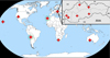 |
Fig. 1 Geographical locations of cameras of AMOS Global Meteor Network. Stations used in this work are indicated with green circles. |
2 Methodology
2.1 The All-Sky Meteor Orbit System
In our work, we investigated the data collected by cameras of the All-Sky Meteor Orbit System (AMOS). AMOS is a project developed at Comenius University in Bratislava, Slovakia and led by Dr. Juraj Tóth (Tóth et al. 2011, 2015, 2019; Zigo et al. 2013). It began as a part of the Slovak Video Meteor Network with the first prototype developed in 2007 at the Astronomical and Geophysical Observatory in Modra, Slovakia. Since then, it has spread across Slovakia and the rest of the world, forming the AMOS Global Meteor Network (Fig. 1), which currently (June 2025) consists of 17 standard AMOS cameras and 17 AMOS-Spec-HR spectral systems (Matlovič et al. 2020). AMOS is an autonomous, intensified video system for the detection of transient sky events, developed mainly for the purpose of observing meteors. The basic optical components of the AMOS system include an all-sky fisheye lens, image intensifier, projecting lens, and a digital CCD video camera (Zigo et al. 2013). The remotely operated camera is hidden in an opening weatherproof enclosure that is connected to a computer with its own software, access to the Internet, and sensors of external meteorological parameters. The field of view of the camera is 180°x140° with a resolution of 1600x1200 px (6.8 arcmin/px) and 20 FPS recording (or 1280x960 px and 15 FPS for older stations in Slovakia). The limiting magnitude is +5.5m for stars and +4m for moving objects. Each location has at least two cameras situated 80 to 150 km from each other. In addition to the observation cameras, there are slitless spectroscopic cameras (AMOS-Spec-HR) with a resolution of 2048x1536 px, spectral resolution of 0.5 nm/px, 20 FPS recording, field of view of 60° × 45°, and a limiting magnitude of +3m for meteors and −1.5m for spectral events (Matlovič et al. 2019, 2020).
The AMOS is operated by its own software AMOS 1.3.4 written in C++, which is used for image processing, transient sky event and star detection, and image/video exportation. The all-sky astrometric reduction and photometric reduction were performed using the method of Borovička et al. (1995) performed in the original Meteor Trajectory (MT) software developed by Kornoš et al. (2015, 2018). Apparent magnitudes of a meteor in each frame were corrected for the distance, atmospheric extinction and vignetting to obtain the light curve in absolute magnitudes. Meteor trajectory calculation was performed in MT using two different methods of Ceplecha (1987) and Borovička (1990). For the luminous efficiency, the software has five implemented models according to Ceplecha & McCrosky (1976); Pecina & Ceplecha (1983); Halliday et al. (1996); Hill et al. (2005), and Weryk & Brown (2013).
Material strength classification of meteoroids based on KB, kc, and PE empirical parameters.
2.2 Dataset and selection criteria
We analyzed two databases collected by the AMOS doublestation cameras located on the Canary Islands and in Chile (Fig. 1). The AMOS Canary database originally contained data concerning 2107 events collected in 2015, and the AMOS Chile database contained 1890 cases detected in 2016. The databases were first sorted to remove false positives, cases with unrealistic physical parameters and hyperbolic meteors. Meteors with hyperbolic orbits usually indicate inaccuracies in data, but they could also originate from the Oort cloud due to interstellar perturbations (Hajdukova et al. 2020; Peña-Asensio et al. 2024). As we did not want to discard interesting cases that could be among hyperbolic meteors, we set a 1.1 upper sorting limit for eccentricity. The aforementioned sorting procedures reduced the numbers of meteors to 1933 for the Canary database and 1728 for the Chile database. Statistical graphs with data on chosen physical parameters for the whole sorted databases are provided in Appendix A.
The material of meteoroids was assessed calculating empirical criteria, which are used to quantify the material strength of meteoroids by the one-dimensional parameterization of collected meteor data (Ceplecha 1958, 1967; Ceplecha & McCrosky 1976; Borovička et al. 2022a; Jenniskens 2023). Meteoroids’ ability to penetrate the atmosphere is linked to their material strength, which is itself determined by the composition of meteoroid (Borovička 2006; Popova et al. 2011; Jenniskens et al. 2024a). Fragile particles crumble earlier, whereas stronger materials can withstand higher pressures and reach lower parts of the atmosphere before fragmentation. Ceplecha (1958) studied the relation between thermal conductivity properties of small (mm to cm-sized) meteoroids and their penetration ability through the atmosphere. The author assumed that all meteoroids begin to be luminous at the same surface temperature. By separating the solution to the heat-conductivity problem for the surface temperature during the beginning part of the meteor trajectory into the left side dependent only on material constants and the right side dependent only on distantly measurable quantities and rewriting it in logarithmic form, Ceplecha (1958) obtained a convenient representation of material properties of a meteoroid, KB, as a function of its beginning height (Eq. (1)). Jenniskens (2023) and Jenniskens et al. (2024b) conducted complex studies of meteor showers, including the distribution of their initial heights. The authors defined the beginning height parameter, kc (with dimensions of [km], valid for meteors with absolute magnitudes M = 0), which they used to categorize meteor showers into several height types associated with material of parent bodies (Eq. (2), Table 2).
Ceplecha & McCrosky (1976) studied fireball end heights and noticed that large meteoroids with similar observed properties had different penetration heights. They linked this observation with meteoroid material strength and introduced another empirical parameter, PE, used for fireball-producing meteoroids (Eq. (3)). Studying the relation between dynamic pressure acting on meteoroids and their material strength, Borovička et al. (2022a) derived a new empirical criterion, which they called the pressure resistance factor Pf . The authors compared dependencies of Pf and PE on different measured quantities (mass, velocity, trajectory slope, atmospheric density) and from that derived the modified PE criterion (Eq. (4)), which is more physically accurate than the original PE.
Parameters used in our work are defined as follows:
 (1)
(1)
 (2)
(2)
 (3)
(3)
 (4)
where hb is the beginning height of a meteor (in km), ρb/ρe is the atmospheric density (in g/cm3) at the beginning or end height, v∞ is the pre-atmospheric (beginning) velocity (in cm/s for KB and in km/s for kc and PE), zR is the zenith distance of the apparent radiant of the meteor, and m76 is the photometric mass (in g) calculated using the specific luminous efficiency defined in Ceplecha & McCrosky (1976). Atmospheric densities were obtained from the atmospheric model NRLMSISE-00 (Picone et al. 2002).
(4)
where hb is the beginning height of a meteor (in km), ρb/ρe is the atmospheric density (in g/cm3) at the beginning or end height, v∞ is the pre-atmospheric (beginning) velocity (in cm/s for KB and in km/s for kc and PE), zR is the zenith distance of the apparent radiant of the meteor, and m76 is the photometric mass (in g) calculated using the specific luminous efficiency defined in Ceplecha & McCrosky (1976). Atmospheric densities were obtained from the atmospheric model NRLMSISE-00 (Picone et al. 2002).
According to Ceplecha (1988), meteors and fireballs can be categorized in several groups based on values of KB and PE parameters. These taxonomic groups (from the strongest to the weakest) are shown in Table 2, together with the kc groups of Jenniskens (2023). For our purposes, following this classification and using the values of modified PE2 (Eq. (4)), we divided meteoroids in our sample into asteroidal or rocky (Type I, with PE,mod > −4.6) and cometary or volatile-rich (Types II and III, PE,mod < −4.6). The PE taxonomy was chosen since it is more frequently used in the literature (Moreno-Ibáñez et al. 2020; Vida et al. 2023) and because the KB classification is depended on sensitivity of detectors (Koten et al. 2004), whereas the kc classification was introduced for shower meteors with a specific condition of M = 0 (Jenniskens 2023).
To avoid “contamination” with the material originating from comets, we excluded major and established meteor showers from our dataset, focusing mainly on sporadic meteors or meteors from non-confirmed minor showers (Jopek & Kaňuchová 2017). We restricted our studies to sporadic meteors because we were interested in larger “independent” bodies of “macroscopic” sizes, which we assumed were not significantly affected by space weathering and other altering processes.
A convenient representation of the orbital type of minor bodies is the Tisserand parameter with respect to Jupiter (Kresák 1979, Kresák 1982; Levison 1996). It is derived from the restricted three-body problem (the Sun, Jupiter, and a small body with negligible mass) and can be defined as
 (5)
where
(5)
where
 (6)
(6)
Here, a, e, i, and Ω are the semi-major axis, eccentricity, orbital inclination, and longitude of the ascending node of a studied object, aJ, iJ, and ΩJ are the corresponding orbital elements of Jupiter, and I is an inclination of the object with respect to Jupiter’s orbital plane3. Using this parameter, we can draw a non-strict border4 between asteroidal and cometary orbits, with TJ > 3 for asteroids and TJ < 3 for comets; that is, specifically TJ < 2 for HTC or LPC cometary orbits (Levison 1996; Jewitt & Hsieh 2022).
TJ is only defined for elliptical orbits, so it is not appropriate to use Eq. (5) for hyperbolic meteors. For such cases, we redefined their eccentricities to be close to unity. Semi-major axes were expressed through the known values of perihelion distances, q, from the database and the defined e. Inserting these values into Eq. (5), we obtained a relation for hyperbolic orbits:
 (7)
(7)
For the determination of meteoroid mass, we used the photometric method, which is based on the assumption that a fraction of the meteoroid kinetic energy is transformed into radiation during the meteor flight. Photometric mass is found by measuring this radiated energy (or luminosity), I, along the meteor trail. The luminosity equation is
 (8)
where t is time, v is velocity, m is meteoroid mass, and τ is luminous efficiency (Ceplecha et al. 1998). In most cases, the energy loss is dominated by the first term (mass loss). The photometric mass was calculated by omitting the second term and integrating the total observed light production (neglecting the terminal mass):
(8)
where t is time, v is velocity, m is meteoroid mass, and τ is luminous efficiency (Ceplecha et al. 1998). In most cases, the energy loss is dominated by the first term (mass loss). The photometric mass was calculated by omitting the second term and integrating the total observed light production (neglecting the terminal mass):
 (9)
(9)
Meteor brightness is measured in absolute visual magnitude, M, which we converted to luminosity by
 (10)
where I0 is the energy of a zero-magnitude meteor, which depends on the particular spectral band (Ceplecha et al. 1998; Borovička et al. 2020). For the luminous efficiency, τ(v) according to Pecina & Ceplecha (1983) was used.
(10)
where I0 is the energy of a zero-magnitude meteor, which depends on the particular spectral band (Ceplecha et al. 1998; Borovička et al. 2020). For the luminous efficiency, τ(v) according to Pecina & Ceplecha (1983) was used.
In this work, we were looking for Type I rocky meteoroids (PE classification) on cometary orbits with TJ < 2 (including Halley-type orbits, since long-period orbits of meteroids can evolve to have lower semi-major axes). We were primarily targeting larger meteoroids (to distinguish them from small cometary inclusions) similar to the cases listed in Table 3. For meteoroid mass, we used two different upper limits: 10 g, following Vida et al. (2023), in order to compare with their results; and 1 g, for which we had only data from AMOS. We did not limit other parameters (except for beginning velocity, for which we applied a lower limit of 50 km/s following Vida et al. (2023); however, see discussion in Sect. 3), instead looking through each selected case manually. The quality of data was subsequently checked based on values of cross angles (angle between two planes that cross the meteor trajectory and the station), percentage of meteor trajectory commonly seen by both stations, numbers of observed points, meteor duration, radiant and velocity uncertainties (the most significant sources of inaccuracies; see Hajduková & Kornoš 2020), and so on. The overall quality of individual cases was judged based on acceptable values of parameters known from previous experience and from the literature. For uncertain cases, we also checked the original images of the meteor and behavior of the light curve.
2.3 Meteor flux
The flux of meteoroids in the Earth’s atmosphere, F, is defined as a number of meteoroids passing through a unit of area in a unit of time, down to a specified mass limit, mlim:
 (11)
(11)
where N(m > mlim) is the number of meteoroids which have mass greater than mlim, Aeff is the effective area of the atmosphere observed by the detecting system at a given height, and tobs is the total observational time (Vida et al. 2022). The product Aeff · tobs is referred to as the total time-area product. For independent multiple-station observations (i.e., from different meteor networks), numbers of events, N, and time-area products for each station were added (but not the fluxes themselves).
To calculate the flux, we needed to know time-area products, Aeff · tobs, for analyzed databases. The AMOS Canary database contains data concerning meteors observed between 1 June, 2015 and 26 December, 2015; that is, 208 nights in total. The AMOS Chile database contains data collected from 21 March, 2016 to 24 November, 2016, giving 248 nights of observations. The estimated total observational times are 990.5 hours for AMOS Canary stations and 1441.25 hours for AMOS Chile stations (see Kuksenko & Tóth (2025) for details). The effective area was calculated for the height of 70 km above the sea level in order to be consistent with Halliday et al. (1996) and Vida et al. (2023). One AMOS camera sees ~392 000 km2 at this altitude (neglecting insignificant differences between altitudes of locations of AMOS Canary and Chile stations). Combining single-camera areas seen by each of the two stations with known separation between them, we obtained estimates of effective areas (area seen by both stations simultaneously) for double-station observations. The resulting values are ~341 000 km2 for AMOS Canary stations and 363 000 km2 for AMOS Chile stations (see Kuksenko & Tóth (2025) for the estimation procedures). This gave us time-area products of ~337 760 500 km2·h for the Canary database and ~523 173 750 km2·h for the Chile database.
For the uncertainty estimates, we assumed that meteor events are random, independent, and distributed according to the Poisson statistical distribution. Then, the uncertainty for the number of events, N, was estimated as a 95% confidence interval of the Poisson distribution, with the upper and lower bounds of the interval calculated by the following formulas:
![Mathematical equation: ${N_{upper}} = 0.5 \cdot {\chi ^2}\left[ {2\left( {N + 1} \right),1 - {\alpha \over 2}} \right],$](/articles/aa/full_html/2025/12/aa55020-25/aa55020-25-eq13.png) (12)
(12)
![Mathematical equation: ${N_{lower}} = 0.5 \cdot {\chi ^2}\left[ {2N,{\alpha \over 2}} \right],$](/articles/aa/full_html/2025/12/aa55020-25/aa55020-25-eq14.png) (13)
where χ2 [ ] is the percent point function of the χ2 distribution, α = 0.05 is the significance level for 95% confidence level (Ulm 1990). For case Nast = 0, the one-sided 95% confidence interval [0; 2.9957] was used5. To estimate the 95% confidence intervals for the fluxes, we inserted Nupper and Nlower values into Eq. (11) instead of N, obtaining Fupper and Flower bounds for fluxes.
(13)
where χ2 [ ] is the percent point function of the χ2 distribution, α = 0.05 is the significance level for 95% confidence level (Ulm 1990). For case Nast = 0, the one-sided 95% confidence interval [0; 2.9957] was used5. To estimate the 95% confidence intervals for the fluxes, we inserted Nupper and Nlower values into Eq. (11) instead of N, obtaining Fupper and Flower bounds for fluxes.
Physical properties and orbital and trajectory parameters of a group of large Type I meteoroids originating in the Oort cloud found in the literature.
3 Results
3.1 Results of the search for dense meteoroids
In this section, we describe the results on the objects found in our databases that fulfilled selection criteria described in Sect. 2.2. In total, we selected 44 meteors from the Canary database and 18 meteors from the Chile database, with TJ < 2 and m > 1 g. Among them, there were two asteroidal and 42 cometary Canary meteoroids and five asteroidal and 11 cometary Chile meteoroids (plus 2 asteroidal with m > 10 g, but with less reliable data), according to Ceplecha (1988) material classification. Peaks of absolute visual magnitudes of chosen meteors lay in a range of approximately +1m to −11.5m. Detailed properties of the selected cases can be found in Kuksenko & Tóth (2025).
In Fig. 2, we compare penetration heights of selected meteors from two databases as a function of velocity. The initial idea was based on the assumption that for faster meteoroids it is harder to penetrate lower into the atmosphere, so meteors with both high velocities and low penetration heights should be denser than usual. As we can see, meteoroids of stronger composition indeed penetrated deeper into the atmosphere, as expected. For comparison, the typical terminal heights of cometary meteoroids are ~80−120 km, depending on the beginning velocity (Borovička et al. 2002; Koten et al. 2004), which is also in agreement with Fig. 2. We can also see from the figure that the beginning height was less representative in determining the material of our selected meteoroids, since more than half of the cases designated as “asteroidal” by us belong to weaker II and III kc beginning height classes.
Vida et al. (2023) set the limit of 50 km/s to remove observational bias toward the more massive meteor-producing objects in the low-speed regime (Hajdukova et al. 2020). However, most of the rocky meteors found were significantly slower (only one case faster than 50 km/s), so we did not limit velocities of asteroidal meteors. There are no physical limitations for velocity for the Oort cloud objects, since they are distributed isotropically and can come to the Earth from any direction (Oort 1950). Still, to ensure consistency with Vida et al. (2023), we applied a 50 km/s limit to cometary cases, which resulted with the seeming distinction between the two material types seen in Fig. 2.
In our work, we took values of PE,mod as a primary criterion for meteoroid material, as it is more reliable for fireball-producing meteoroids. However, we also tried to compare it with other material parameters (Figs. 2–4). It can be noticed from the graphs that different classifications give slightly different results for meteoroid composition. The most problematic are cases on the boundaries of types which are defined empirically. Deviations of measurements can shift meteoroids to neighboring material types. We do not show the uncertainties of TJ in our graphs, since they are quite large for some cases and do not fit within the given scale.
For the meteoroid mass, we used the photometric mass calculated with the luminous efficiency τ according to Pecina & Ceplecha (1983). Although there are more modern models for τ with the mass dependency included (Revelle & Ceplecha 2001; Borovička et al. 2020; Vida et al. 2024), they have not yet been incorporated into the MT software, so we used the mass scale that is the closest to modern models, keeping in mind that the resulting masses can be under- or overestimated (this is a general problem with the luminous efficiency). We only found two rocky meteors with mphot > 10 g satisfying our criteria, but with low data quality (small convergence angles and high mass errors). Because of the mentioned inaccuracies, we did not consider these two meteors in our further calculations. Among cometary meteors, five cases have mphot > 10 g, all of which are from the Canary database. The remaining selected meteoroids have smaller masses (between 1 and 10 g), corresponding to ~1 cm. This mass regime is close to Karlštejn-like and smaller rocky meteoroids, but also to the largest known refractory inclusions in comets (Brownlee 2014; Davidsson et al. 2016; Paquette et al. 2016).
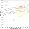 |
Fig. 2 Beginning velocities versus beginning and end heights of selected asteroidal and cometary meteoroids with uncertainties (gray bars). Marker represents the database. Lines correspond to borders between kc beginning height classes according to Jenniskens (2023) provided in Table 2. |
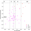 |
Fig. 3 KB material parameters versus Tisserand parameters of selected asteroidal (red) and cometary (magenta) meteoroids on Halley-type (HP) and long-period (LP) cometary orbits. Color represents the PE material classification. Marker represents the database. Uncertainties in KB are shown via gray bars. |
3.2 Meteor flux and ice-to-rock ratio estimates
We calculated fluxes of rocky and cometary meteoroids on cometary orbits for two mass limits: 10 and 1 g. For the 10 g mass regime, we tried several data combinations. From the AMOS data, we had five cometary meteoroids in the Canary database and no asteroidal meteoroids with reliable data6. These numbers were inserted into Eq. (11), together with the corresponding time-area products estimated in Sect. 2.3. The resulting fluxes were converted into units of meteoroids per 106 km2 per year. The population of rocky meteoroids in the Oort cloud was then estimated as the ratio of the asteroidal flux Fast to the total flux Fast + Fcom. The upper and lower bounds of the 95% confidence interval for the rocky population were calculated by substituting the asteroidal fluxes with upper and lower bounds of Fast. The results are provided in Table 4.
For the 1 g mass limit, we only had data from AMOS. The obtained population of rocky meteoroids in the Oort cloud heavier than 1 g is 11.7% (~5.1 – 21.4%). For the 10 g rocky population, we obtained the result of ~0–19%. Since cometary meteoroids with a 10 g mass limit were observed only by Canary cameras, the Canary time-area product for the cometary flux was used. Although we used zero as a number of observed rocky meteoroids in this case (which is also a result on its own), we could still extract some useful information, even if it does not tell us much given the high uncertainty of the result.
Next, we tried to combine our results with the results of Vida et al. (2023), which are also provided in Table 4 for comparison. We tried two combinations – including only cometary cases observed by the AMOS system, and incorporating our results concerning the non-observation of reliable rocky meteoroids. In the first combination, the time-area product of Vida et al. (2023) for cometary flux was expanded by the AMOS Canary time-area product, and the numbers of cometary meteoroids were combined. This approach resulted in a 5.3% (~0.7−16.8%) population of rocky meteoroids in the Oort cloud, reducing the nominal 6.0% (~0.8−18.8%) population originally estimated by Vida et al. (2023). In the second combination, we truncated the results of Vida et al. (2023) even more by changing the asteroidal flux as well. We did it by “adding” zero rocky meteoroids from the AMOS system to two rocky meteoroids used by Vida et al. (2023) and expanding the asteroidal time-area product correspondingly. By doing that, we managed to reduce the original result for the rocky population in the Oort cloud to 5% (~0.6−16.1%).
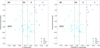 |
Fig. 4 Comparison between PE and modified PE material parameters of selected asteroidal (blue) and cometary (cyan) meteoroids on Halley-type (HP) and long-period (LP) cometary orbits. Color represents the PE material classification (according to values of PE,mod). Marker represents the database. Uncertainties in PE are shown by gray bars. |
Results of flux and population of refractory objects in the Oort cloud calculations.
4 Discussion
One may question how representative and complete our dataset for chosen mass limits is. The AMOS data are not “clear-sky” data as those from the MORP survey (Halliday et al. 1996). It means that the best approach is not to completely trust the software and to check every unusual case manually for confidence. However, our selection process of interesting meteors could be subjective in many terms, depending on a human factor and imperfections of the dataset. Our numbers could be corrected by theoretical predictions of the Oort cloud meteoroid population using the mass and population indices (McKinley 1961; Brown & Rendtel 1996), but we are lacking observational data due to the scarcity of such objects. This is where studies of fluxes in smaller mass regimes (such as our 1 g population) may be useful.
Regarding the orbital classification, the determination of orbital parameters, especially the semi-major axis, is highly dependent on the quality of measurements of radiant position and beginning velocity (Hajdukova et al. 2020; Hajduková & Kornoš 2020). For meteors with large a and e, even a small uncertainty in the measured velocity transfers to a large uncertainty in the semi-major axis. Unfortunately, such errors are inevitable given the quality of meteor measurements by video observations (Hajduková & Kornoš 2020). Large a errors are transferred to the calculated errors of TJ, on which we based our orbital classification. Some errors in TJ are so large that the determination of orbital type with this method becomes questionable. However, it is worth mentioning that the Tisserand parameter is an imperfect criterion, which is used mostly as a first approximation of an orbital type (Jewitt & Hsieh 2022).
We would wish to know whether the selected meteoroids are primordial and if they can be treated as independent objects left after the formation of the Solar System. However, we cannot be certain when considering the masses of these meteoroids: they are too small to be treated as macroscopic (as the parent body of the Alberta fireball), but relatively large compared to refractory inclusions in comets. Comets themselves may be collisional rubble piles made of processed material, although modern studies suggest that they are mostly primordial bodies (Davidsson et al. 2016). If such refractory meteoroids are fragments of larger rocky bodies, the question of how they got to the Oort cloud remains.
Considering the number of non-gravitational effects affecting the orbits of such small objects and thermal and space weathering effects affecting their composition, it is hard to use a population of ~1 g objects in terms of cosmogony of the early evolutionary stages of the Solar System. However, Jenniskens et al. (2024a) claimed that this population should still reflect the composition of primordial protoplanetary disk pebbles from which the Oort cloud formed, and that space weathering did not play a significant role in changing of their composition throughout the later evolutionary stages of the Solar System. The authors suggested that these “former” pebbles were thermally altered by the young Sun heating them high above and below the primordial disk plane. This mechanism can potentially explain the existence of the present ~1 g refractory population.
Regarding meteor fluxes, our results from different combinations of data yielded the percentages listed below:
~11.7% of rocky meteoroids out of total number of objects in the Oort cloud with masses larger than 1 g (AMOS data).
~0−19% of refractory meteoroids in the Oort cloud with masses larger than 10 g (AMOS data).
~5.3% of the 10 g refractory population (data of Vida et al. (2023), combined with cometary flux observed by the AMOS system).
~5% of the 10 g rocky population (combined Vida et al. (2023) and AMOS complete data).
The AMOS data fluxes are larger compared to Vida et al. (2023), because our system performed observations over a shorter period of time, but this fact is compensated by broader uncertainty intervals. Flux calculation is the most sensitive to effective area errors (Vida et al. 2022). However, given that the AMOS time-area products are 10−100 times smaller than the MORP and GFO combined product, we did not include the uncertainties in time and area in our calculation, because the combined fluxes are dominated by the data of Vida et al. (2023); the authors did not include these errors in their calculations either.
Our resulting population of ~1 g refractory particles (mm– cm size domain) is larger than the 4% observed by Jenniskens et al. (2024a). If our results are correct, it could mean that the mechanism proposed by Jenniskens et al. (2024a) may not be enough to explain the size of rocky particles’ population in this mass regime, and that gravitational perturbations causing material mixing across the Solar System must also have been involved. However, given the large uncertainties of our fluxes, we will need more observations to provide definite answers. Moreover, the authors studied meteor showers, whereas we excluded showers and concentrated on sporadic background. Since there are no published estimates in a similar mass regime of sporadic meteors, we cannot directly compare our 1 g results with those of other authors.
Our combined results in the 10 g mass regime are more interesting. Using our AMOS data, we managed to truncate the original results of Vida et al. (2023). Our result, although smaller, still agrees with the conclusions of the authors: among cosmogonic models mentioned in Table 1, the closest comparable prediction to our estimated ~5% is given by the Grand Tack model (Walsh et al. 2011; Shannon et al. 2019). However, if we also consider uncertainties, the lower bound of the confidence interval for the second combined approach gives ~0.6%, which is close to predictions of Meech et al. (2016) for the cosmogonic models of Weissman & Levison (1997) and Izidoro et al. (2013).
Concerning the large flux uncertainties, since the study was based on the combination of large time-area products from different meteor networks and given that only a few asteroidal cases were detected (e.g., only 2 cases – Karlstein and Alberta – were used in a combined approach in 10 g mass regime), it is natural that Poisson statistical formulas gave us such high uncertainty intervals. More detections of this kind would lower the uncertainties, as we show with our combined approach.
The mentioned comparison of predictions and observations together with the problem of high uncertainties raise a fair question as to whether such comparisons are even legitimate and whether they tell us anything definite about the evolutionary history of the Solar System, considering the large number of unknown parameters and approximate results of both numerical simulations and meteor observations. Our main conclusion from this comparison is that the methods of numerical modelling should be improved to reduce the uncertainties and to obtain more definitive constraints. From the observational side, it is important to continue small-body and meteor observations due to small number of observed unusual events. A good approach is to combine data from different meteor databases and authors. For example, it would be interesting to incorporate data from the European fireball network (Oberst et al. 1998), Finnish Fireball Network (Gritsevich et al. 2014) and CAMS project (Jenniskens et al. 2011), including the mentioned Karlštejn and FH1 fireballs, and the results of Jenniskens et al. (2024a).
We should emphasize that the empirical classifications used give only approximate information about the meteoroid composition and should not be taken strictly. More complete information can be obtained from spectral observations and laboratory analysis of meteorite recoveries, which can be used to calibrate other methods.
5 Conclusions
The aim of this work was to show how studies of physical properties of meteoroids can be applied in the field of planetary cosmogony of the Solar System. We analyzed meteor data collected by the cameras of the AMOS located on the Canary Islands and in Chile. A multiparameter approach was used to search for refractory meteoroids on Halley-type and long-period cometary orbits with mass larger than 1 g in our databases. In addition to the material (classified using the modified PE criterion) and orbits (based on the Tisserand parameter values), we checked meteoroids for their beginning velocities, end heights, and various other parameters, searching for strong meteoroids that penetrated deep into the Earth’s atmosphere. Our selection process yielded 44 meteors from the Canary database (2 refractory and 42 cometary cases) and 18 meteors from the Chile database (7 refractory and 11 cometary cases). Among the selected cases, two asteroidal meteoroids and five cometary meteoroids had masses larger than 10 g. However, further analysis showed the low quality of the data on the two 10 g asteroidal meteoroids found, so they were excluded from our calculations.
Our main idea was to use the ratio of asteroidal and total meteor fluxes as a proxy for the ice-to-rock ratio of the Oort cloud – the key observational constraint used in this work for testing cosmogonic models of the Solar System. We calculated asteroidal and cometary meteor fluxes based on the observed numbers of meteors and known time-area products for the studied databases. The obtained fluxes were subsequently used to evaluate the percentage of the refractory component of the Oort cloud. The population of rocky objects in the Oort cloud with masses larger than 1 g was estimated to be ~11.7%. The refractory population of the Oort cloud with masses larger than 10 g is ~5%.
With our combined approaches, we managed to truncate previous ~6% estimate of Vida et al. (2023) for the ~10 g refractory component of the Oort cloud. We showed that it is possible to constrain the population of rocky objects in the Oort cloud even without any reliable detections, just using known time-area products and detections of cometary meteoroids. Our results combined with those of other authors agree with the predictions of the migration-based Grand Tack cosmogonic model, suggesting that the primordial material left after the Solar System formation could have been more mixed than was previously thought.
In future works on this topic, further development of numerical simulations with more accurate theoretical predictions and the derivation of more precise orbital and material classifications of meteoroids will be beneficial. From the observational side, improvement of data quality of video systems observing meteors is highly desirable. Our general conclusion is that the studied topic has potential for further research. The shown methodology can be used by other authors with improvements. Our results can be combined with data from other AMOS databases or from different meteor networks. Further studies can involve meteoroids of lower mass regimes and meteoroids originating from shower-producing streams. The results on meteor fluxes can also be used in general studies of small Solar-System bodies, their orbital and material evolution, as well as in testing models of comets and the Oort cloud formation.
Acknowledgements
This work was supported by the Slovak Grant Agency for Science (grant VEGA 1/0218/22), the Slovak Research and Development Agency grants APVV-16-0148 and APVV-23-0323, and by COST (European Cooperation in Science and Technology; www.cost.eu) within the framework of COST Action CA22133 - The birth of solar systems (PLANETS). We would also like to express our gratitude to Dr. Denis Vida, who kindly shared his Python code to help with the uncertainty estimates of the final results.
Reference
- Borovička, J. 1990, Bull. Astron. Inst. Czechoslovakia, 41, 391 [NASA ADS] [Google Scholar]
- Borovička, J. 2006, IAU Symp., 229, 249 [Google Scholar]
- Borovička, J., Spurný, P., & Keclíková, J. 1995, A&AS, 112, 173 [Google Scholar]
- Borovička, J., Spurný, P., & Koten, P. 2002, ESA SP, 500, 265 [Google Scholar]
- Borovička, J., Koten, P., Spurný, P., Boček, J., & Štork, R. 2005, Icarus, 174, 15 [CrossRef] [Google Scholar]
- Borovička, J., Spurný, P., & Shrbený, L. 2020, AJ, 160, 42 [CrossRef] [Google Scholar]
- Borovička, J., Spurný, P., & Shrbený, L. 2022a, A&A, 667, A158 [NASA ADS] [CrossRef] [EDP Sciences] [Google Scholar]
- Borovička, J., Spurný, P., Shrbený, L., et al. 2022b, A&A, 667, A157 [NASA ADS] [CrossRef] [EDP Sciences] [Google Scholar]
- Brasser, R., & Morbidelli, A. 2013, Icarus, 225, 40 [Google Scholar]
- Brown, P., & Rendtel, J. 1996, Icarus, 124, 414 [Google Scholar]
- Brownlee, D. 2014, Ann. Rev. Earth Planet. Sci., 42, 179 [Google Scholar]
- Ceplecha, Z. 1958, Bull. Astron. Inst. Czechoslovakia, 9, 154 [NASA ADS] [Google Scholar]
- Ceplecha, Z. 1967, Smith. Contrib. Astrophys., 11, 35 [Google Scholar]
- Ceplecha, Z. 1987, Bull. Astron. Inst. Czechoslovakia, 38, 222 [NASA ADS] [Google Scholar]
- Ceplecha, Z. 1988, Bull. Astron. Inst. Czechoslovakia, 39, 221 [NASA ADS] [Google Scholar]
- Ceplecha, Z., & McCrosky, R. E. 1976, J. Geophys. Res., 81, 6257 [NASA ADS] [CrossRef] [Google Scholar]
- Ceplecha, Z., Borovička, J., Elford, W. G., et al. 1998, Space Sci. Rev., 84, 327 [NASA ADS] [CrossRef] [Google Scholar]
- Chapman, C. R. 1996, Meteor. Planet. Sci., 31, 699 [NASA ADS] [CrossRef] [Google Scholar]
- Chapman, C. R. 2004, Ann. Rev. Earth Planet. Sci., 32, 539 [Google Scholar]
- Davidsson, B. J. R., Sierks, H., Güttler, C., et al. 2016, A&A, 592, A63 [NASA ADS] [CrossRef] [EDP Sciences] [Google Scholar]
- DeMeo, F. E., Binzel, R. P., Slivan, S. M., & Bus, S. J. 2009, Icarus, 202, 160 [Google Scholar]
- Devillepoix, H. A. R., Cupák, M., Bland, P. A., et al. 2020, Planet. Space Sci., 191, 105036 [Google Scholar]
- Flynn, G. J., Consolmagno, G. J., Brown, P., & Macke, R. J. 2018, Chemie der Erde / Geochem., 78, 269 [Google Scholar]
- Giorgini, J. D., Yeomans, D. K., Chamberlin, A. B., et al. 1996, AAS/Div. Planet. Sci. Meeting Abstracts, 28, 25.04 [Google Scholar]
- Gomes, R., Levison, H. F., Tsiganis, K., & Morbidelli, A. 2005, Nature, 435, 466 [Google Scholar]
- Gounelle, M., Morbidelli, A., Bland, P. A., et al. 2008, in The Solar System Beyond Neptune, eds. M. A. Barucci, H. Boehnhardt, D. P. Cruikshank, A. Morbidelli, & R. Dotson (Tucson: University of Arizona Press), 525 [Google Scholar]
- Gritsevich, M., Lyytinen, E., Moilanen, J., et al. 2014, in Proceedings of the International Meteor Conference, Giron, France, 18-21 September 2014, eds. J. L. Rault, & P. Roggemans, 162 [Google Scholar]
- Hajduková, M., & Kornoš, L. 2020, Planet. Space Sci., 190, 104965 [CrossRef] [Google Scholar]
- Hajdukova, M., Sterken, V., Wiegert, P., & Kornoš, L. 2020, Planet. Space Sci., 192, 105060 [NASA ADS] [CrossRef] [Google Scholar]
- Halliday, I., Griffin, A. A., & Blackwell, A. T. 1996, Meteor. Planet. Sci., 31, 185 [NASA ADS] [CrossRef] [Google Scholar]
- Harvey, G. A. 1974, AJ, 79, 333 [Google Scholar]
- Hill, K. A., Rogers, L. A., & Hawkes, R. L. 2005, A&A, 444, 615 [NASA ADS] [CrossRef] [EDP Sciences] [Google Scholar]
- Hsieh, H. H., & Jewitt, D. 2006, IAU Symp., 229, 425 [NASA ADS] [Google Scholar]
- Izidoro, A., de Souza Torres, K., Winter, O. C., & Haghighipour, N. 2013, ApJ, 767, 54 [NASA ADS] [CrossRef] [Google Scholar]
- Jenniskens, P. 2023, Atlas of Earth’s Meteor Showers (Amsterdam: Elsevier) [Google Scholar]
- Jenniskens, P., Gural, P. S., Dynneson, L., et al. 2011, Icarus, 216, 40 [NASA ADS] [CrossRef] [Google Scholar]
- Jenniskens, P., Estrada, P. R., Pilorz, S., et al. 2024a, Icarus, 423, 116229 [Google Scholar]
- Jenniskens, P., Pilorz, S., Gural, P. S., et al. 2024b, Icarus, 415, 116034 [Google Scholar]
- Jewitt, D. 2012, AJ, 143, 66 [CrossRef] [Google Scholar]
- Jewitt, D., & Hsieh, H. H. 2022, arXiv e-prints [arXiv:2203.01397] [Google Scholar]
- Jopek, T. J., & Kaňuchová, Z. 2017, Planet. Space Sci., 143, 3 [NASA ADS] [CrossRef] [Google Scholar]
- Kaib, N. A., & Quinn, T. 2008, Icarus, 197, 221 [NASA ADS] [CrossRef] [Google Scholar]
- Kikwaya, J. B., Campbell-Brown, M., & Brown, P. G. 2011, A&A, 530, A113 [NASA ADS] [CrossRef] [EDP Sciences] [Google Scholar]
- Kornoš, L., Ďuriš, F., & Tóth, J. 2015, in International Meteor Conference Mistelbach, Austria, ed. J. L. Rault & P. Roggemans, 101 [Google Scholar]
- Kornoš, L., Duriš, F., & Tóth, J. 2018, in International Meteor Conference, Petnica, Serbia, eds. M. Gyssens, & J.-L. Rault, 46 [Google Scholar]
- Koten, P., Borovička, J., Spurný, P., Betlem, H., & Evans, S. 2004, A&A, 428, 683 [NASA ADS] [CrossRef] [EDP Sciences] [Google Scholar]
- Kresák, L. 1982, Bull. Astron. Inst. Czechoslovakia, 33, 104 [Google Scholar]
- Kresák, L. 1979, in Asteroids, eds. T. Gehrels, & M. S. Matthews (Tucson: University of Arizona Press), 289 [Google Scholar]
- Kuksenko, V., & Tóth, J. 2025, J. Int. Meteor Organiz., 53, 4 [Google Scholar]
- Lambrechts, M., & Johansen, A. 2012, A&A, 544, A32 [NASA ADS] [CrossRef] [EDP Sciences] [Google Scholar]
- Levison, H. F. 1996, ASP Conf. Ser., 107, 173 [NASA ADS] [Google Scholar]
- Levison, H. F., Kretke, K. A., & Duncan, M. J. 2015, Nature, 524, 322 [CrossRef] [Google Scholar]
- Licandro, J., Popescu, M., de León, J., et al. 2018, A&A, 618, A170 [NASA ADS] [CrossRef] [EDP Sciences] [Google Scholar]
- Matlovič, P., Tóth, J., Rudawska, R., & Kornoš, L. 2017, Planet. Space Sci., 143, 104 [NASA ADS] [CrossRef] [Google Scholar]
- Matlovič, P., Tóth, J., Rudawska, R., Kornoš, L., & Pisarčíková, A. 2019, A&A, 629, A71 [NASA ADS] [CrossRef] [EDP Sciences] [Google Scholar]
- Matlovič, P., Tóth, J., Kornoš, L., & Loehle, S. 2020, Icarus, 347, 113817 [CrossRef] [Google Scholar]
- McKinley, D.W. R. 1961, Meteor Science and Engineering (New York: McGraw-Hill Book) [Google Scholar]
- Meech, K. J., Yang, B., Keane, J., et al. 2014, AAS/Division Planet. Sci. Meeting Abstracts, 46, 200.02 [Google Scholar]
- Meech, K. J., Yang, B., Kleyna, J., et al. 2016, Sci. Adv., 2, e1600038 [NASA ADS] [CrossRef] [Google Scholar]
- Morbidelli, A. 2005, arXiv e-prints [arXiv:astro-ph/0512256] [Google Scholar]
- Morbidelli, A., Levison, H. F., Tsiganis, K., & Gomes, R. 2005, Nature, 435, 462 [Google Scholar]
- Moreno-Ibáñez, M., Gritsevich, M., Trigo-Rodríguez, J. M., & Silber, E. A. 2020, MNRAS, 494, 316 [Google Scholar]
- Nesvorný, D., Dauphas, N., Vokrouhlický, D., Deienno, R., & Hopp, T. 2024, Earth Planet. Sci. Lett., 626, 118521 [CrossRef] [Google Scholar]
- Oberst, J., Molau, S., Heinlein, D., et al. 1998, Meteor. Planet. Sci., 33, 49 [CrossRef] [Google Scholar]
- Oort, J. H. 1950, Bull. Astron. Inst. Netherlands, 11, 91 [NASA ADS] [Google Scholar]
- Orofino, V. 2022, Universe, 8, 518 [Google Scholar]
- Paquette, J. A., Engrand, C., Stenzel, O., et al. 2016, Meteor. Planet. Sci., 51, 1340 [Google Scholar]
- Peña-Asensio, E., Visuri, J., Trigo-Rodríguez, J. M., et al. 2024, Icarus, 408, 115844 [CrossRef] [Google Scholar]
- Pecina, P., & Ceplecha, Z. 1983, Bull. Astron. Inst. Czechoslovakia, 34, 102 [NASA ADS] [Google Scholar]
- Picone, J. M., Hedin, A. E., Drob, D. P., & Aikin, A. C. 2002, J. Geophys. Res. Space Phys., 107, 1468 [Google Scholar]
- Popova, O., Borovička, J., Hartmann, W. K., et al. 2011, Meteor. Planet. Sci., 46, 1525 [NASA ADS] [CrossRef] [Google Scholar]
- Portegies Zwart, S., Torres, S., Cai, M. X., & Brown, A. G. A. 2021, A&A, 652, A144 [NASA ADS] [CrossRef] [EDP Sciences] [Google Scholar]
- Raymond, S. N., & Morbidelli, A. 2014, IAU Symp., 310, 194 [Google Scholar]
- Revelle, D. O., & Ceplecha, Z. 2001, ESA SP, 495, 507 [NASA ADS] [Google Scholar]
- Scott, E. R. D., Krot, A. N., & Sanders, I. S. 2018, ApJ, 854, 164 [NASA ADS] [CrossRef] [Google Scholar]
- Shannon, A., Jackson, A. P., Veras, D., & Wyatt, M. 2015, MNRAS, 446, 2059 [Google Scholar]
- Shannon, A., Jackson, A. P., & Wyatt, M. C. 2019, MNRAS, 485, 5511 [CrossRef] [Google Scholar]
- Spurný, P., & Borovička, J. 1999a, IAU Colloq., 173, 163 [Google Scholar]
- Spurný, P., & Borovička, J. 1999b, in Meteroids 1998, eds. W. J. Baggaley, & V. Porubcan (Tucson: University of Arizona Press), 143 [Google Scholar]
- Tóth, J., Kornoš, L., Vereš, P., et al. 2011, PASJ, 63, 331 [Google Scholar]
- Tóth, J., Kornoš, L., Zigo, P., et al. 2015, Planet. Space Sci., 118, 102 [CrossRef] [Google Scholar]
- Tóth, J., Šilha, J., Matlovič, P., et al. 2019, in 1st NEO and Debris Detection Conference_ESA2019, 63 [Google Scholar]
- Tsiganis, K., Gomes, R., Morbidelli, A., & Levison, H. F. 2005, Nature, 435, 459 [Google Scholar]
- Ulm, K. 1990, Am. J. Epidemiol., 131, 373 [Google Scholar]
- Vida, D., Blaauw Erskine, R. C., Brown, P. G., et al. 2022, MNRAS, 515, 2322 [NASA ADS] [CrossRef] [Google Scholar]
- Vida, D., Brown, P. G., Devillepoix, H. A. R., et al. 2023, Nat. Astron., 7, 318 [Google Scholar]
- Vida, D., Brown, P. G., Campbell-Brown, M., & Egal, A. 2024, Icarus, 408, 115842 [Google Scholar]
- Vojáček, V., Borovička, J., Koten, P., Spurný, P., & Štork, R. 2019, A&A, 621, A68 [NASA ADS] [CrossRef] [EDP Sciences] [Google Scholar]
- Vokrouhlický, D., Nesvorný, D., & Dones, L. 2019, AJ, 157, 181 [CrossRef] [Google Scholar]
- Walsh, K. J., Morbidelli, A., Raymond, S. N., O’Brien, D. P., & Mandell, A. M. 2011, Nature, 475, 206 [Google Scholar]
- Weissman, P. R., & Levison, H. F. 1997, ApJ, 488, L133 [Google Scholar]
- Weissman, P. R., Bottke, W. F., J., & Levison, H. F. 2002, in Asteroids III, eds. J. Bottke, W. F., A. Cellino, P. Paolicchi, & R. P. Binzel (Tucson: University of Arizona Press), 669 [Google Scholar]
- Weryk, R. J., & Brown, P. G. 2013, Planet. Space Sci., 81, 32 [CrossRef] [Google Scholar]
- Zigo, P., Toth, J., & Kalmancok, D. 2013, in Proceedings of the International Meteor Conference, 31st IMC, La Palma, Canary Islands, Spain, 2012, eds. M. Gyssens & P. Roggemans, 18 [Google Scholar]
Not significantly affected by thermal processing after condensation from the protostellar nebula.
We used it instead of the original PE criterion; boundaries of material groups remain the same, but values are shifted.
The majority of authors neglect Eq. (6) and use the term cos i instead. The difference is negligible.
Modern dynamical models give a more realistic boundary of TJ ≈ 3.05−3.10 (Jewitt & Hsieh 2022).
Two asteroidal meteoroids with mass >10 g were detected by the AMOS Chile cameras, but, due to low data quality, we decided not to use them in our calculations, as was mentioned in previous section.
Appendix A Statistical graphs on the whole dataset
 |
Fig. A.1 Comparison of beginning (orange) and end (blue) heights for the Canary (top) and Chile (bottom) sorted databases. Heights for hyperbolic meteors are shown separately in lighter colors (yellow and cyan respectively). N is the order number of a meteor in the database. |
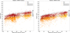 |
Fig. A.2 Statistical graphs of beginning velocities vs beginning and end heights for the AMOS Canary (left) and AMOS Chile (right) sorted databases. Hyperbolic meteors are shown separately in different colors. Lines correspond to borders between kc beginning height classes according to Jenniskens (2023) provided in Table 2 in the main text. |
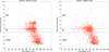 |
Fig. A.3 Statistical graphs of end heights vs Tisserand parameters for the AMOS Canary (left) and AMOS Chile (right) sorted databases. Hyperbolic meteors are shown in dark orange color. Orbital classes according to TJ classification are denoted in gray boxes. Ast stands for asteroidal orbits, JF, HT and LP for Jupiter-family, Halley-type and long-period cometary orbits. |
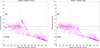 |
Fig. A.4 Statistical graphs of beginning velocities vs Tisserand parameters for two sorted databases. Hyperbolic meteors are in dark purple color. Orbital classes (Ast, JF, HT/LP) are the same as in Fig. A.3. |
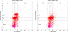 |
Fig. A.5 Statistical graphs of KB material parameters vs Tisserand parameters for two sorted databases. Hyperbolic meteors are shown in magenta color. Orbital classes (Ast, JF, HT/LP) are the same as in Fig. A.3. Material classes (ast, A, B, C, D) are explained in Table 2 in the main text. |
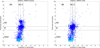 |
Fig. A.6 Statistical graphs of modified PE material parameters vs Tisserand parameters for two sorted databases. Hyperbolic meteors are shown in cyan color. Orbital classes (Ast, JF, HT/LP) are the same as in Fig. A.3. Material classes (I, II, IIIA, IIIB) are explained in Table 2 in the main text. |
All Tables
Cosmogonic models that make predictions of the population of refractory objects in the Oort cloud.
Material strength classification of meteoroids based on KB, kc, and PE empirical parameters.
Physical properties and orbital and trajectory parameters of a group of large Type I meteoroids originating in the Oort cloud found in the literature.
Results of flux and population of refractory objects in the Oort cloud calculations.
All Figures
|
Fig. 1 Geographical locations of cameras of AMOS Global Meteor Network. Stations used in this work are indicated with green circles. |
| In the text | |
|
Fig. 2 Beginning velocities versus beginning and end heights of selected asteroidal and cometary meteoroids with uncertainties (gray bars). Marker represents the database. Lines correspond to borders between kc beginning height classes according to Jenniskens (2023) provided in Table 2. |
| In the text | |
|
Fig. 3 KB material parameters versus Tisserand parameters of selected asteroidal (red) and cometary (magenta) meteoroids on Halley-type (HP) and long-period (LP) cometary orbits. Color represents the PE material classification. Marker represents the database. Uncertainties in KB are shown via gray bars. |
| In the text | |
|
Fig. 4 Comparison between PE and modified PE material parameters of selected asteroidal (blue) and cometary (cyan) meteoroids on Halley-type (HP) and long-period (LP) cometary orbits. Color represents the PE material classification (according to values of PE,mod). Marker represents the database. Uncertainties in PE are shown by gray bars. |
| In the text | |
|
Fig. A.1 Comparison of beginning (orange) and end (blue) heights for the Canary (top) and Chile (bottom) sorted databases. Heights for hyperbolic meteors are shown separately in lighter colors (yellow and cyan respectively). N is the order number of a meteor in the database. |
| In the text | |
|
Fig. A.2 Statistical graphs of beginning velocities vs beginning and end heights for the AMOS Canary (left) and AMOS Chile (right) sorted databases. Hyperbolic meteors are shown separately in different colors. Lines correspond to borders between kc beginning height classes according to Jenniskens (2023) provided in Table 2 in the main text. |
| In the text | |
|
Fig. A.3 Statistical graphs of end heights vs Tisserand parameters for the AMOS Canary (left) and AMOS Chile (right) sorted databases. Hyperbolic meteors are shown in dark orange color. Orbital classes according to TJ classification are denoted in gray boxes. Ast stands for asteroidal orbits, JF, HT and LP for Jupiter-family, Halley-type and long-period cometary orbits. |
| In the text | |
|
Fig. A.4 Statistical graphs of beginning velocities vs Tisserand parameters for two sorted databases. Hyperbolic meteors are in dark purple color. Orbital classes (Ast, JF, HT/LP) are the same as in Fig. A.3. |
| In the text | |
|
Fig. A.5 Statistical graphs of KB material parameters vs Tisserand parameters for two sorted databases. Hyperbolic meteors are shown in magenta color. Orbital classes (Ast, JF, HT/LP) are the same as in Fig. A.3. Material classes (ast, A, B, C, D) are explained in Table 2 in the main text. |
| In the text | |
|
Fig. A.6 Statistical graphs of modified PE material parameters vs Tisserand parameters for two sorted databases. Hyperbolic meteors are shown in cyan color. Orbital classes (Ast, JF, HT/LP) are the same as in Fig. A.3. Material classes (I, II, IIIA, IIIB) are explained in Table 2 in the main text. |
| In the text | |
Current usage metrics show cumulative count of Article Views (full-text article views including HTML views, PDF and ePub downloads, according to the available data) and Abstracts Views on Vision4Press platform.
Data correspond to usage on the plateform after 2015. The current usage metrics is available 48-96 hours after online publication and is updated daily on week days.
Initial download of the metrics may take a while.