| Issue |
A&A
Volume 704, December 2025
|
|
|---|---|---|
| Article Number | A236 | |
| Number of page(s) | 11 | |
| Section | Astrophysical processes | |
| DOI | https://doi.org/10.1051/0004-6361/202555605 | |
| Published online | 12 December 2025 | |
Six binary brown dwarf candidates identified by microlensing
1
Department of Physics, Chungbuk National University, Cheongju 28644, Republic of Korea
2
Korea Astronomy and Space Science Institute, Daejon 34055, Republic of Korea
3
Institute of Natural and Mathematical Science, Massey University, Auckland 0745, New Zealand
4
Astronomical Observatory, University of Warsaw, Al. Ujazdowskie 4, 00-478 Warszawa, Poland
5
University of Canterbury, Department of Physics and Astronomy, Private Bag 4800, Christchurch 8020, New Zealand
6
Department of Astronomy, Ohio State University, 140 West 18th Ave., Columbus, OH 43210, USA
7
University of Science and Technology, Daejeon 34113, Republic of Korea
8
Department of Particle Physics and Astrophysics, Weizmann Institute of Science, Rehovot 76100, Israel
9
Center for Astrophysics | Harvard & Smithsonian 60 Garden St., Cambridge, MA 02138, USA
10
Department of Astronomy and Tsinghua Centre for Astrophysics, Tsinghua University, Beijing 100084, China
11
School of Space Research, Kyung Hee University, Yongin, Kyeonggi 17104, Republic of Korea
12
Department of Physics, University of Warwick, Gibbet Hill Road, Coventry CV4 7AL, UK
13
Villanova University, Department of Astrophysics and Planetary Sciences, 800 Lancaster Ave., Villanova, PA 19085, USA
14
Institute for Space-Earth Environmental Research, Nagoya University, Nagoya 464-8601, Japan
15
Code 667, NASA Goddard Space Flight Center, Greenbelt, MD 20771, USA
16
Department of Astronomy, University of Maryland, College Park, MD 20742, USA
17
Department of Earth and Planetary Science, Graduate School of Science, The University of Tokyo, 7-3-1 Hongo, Bunkyo-ku, Tokyo 113-0033, Japan
18
Instituto de Astrofísica de Canarias, Vía Láctea s/n, E-38205 La Laguna, Tenerife, Spain
19
Department of Earth and Space Science, Graduate School of Science, Osaka University, Toyonaka, Osaka 560-0043, Japan
20
Department of Physics, The Catholic University of America, Washington, DC 20064, USA
21
Institute of Astronomy, Graduate School of Science, The University of Tokyo, 2-21-1 Osawa, Mitaka, Tokyo 181-0015, Japan
22
Institute of Space and Astronautical Science, Japan Aerospace Exploration Agency, 3-1-1 Yoshinodai, Chuo, Sagamihara, Kanagawa 252-5210, Japan
23
Sorbonne Université, CNRS, UMR 7095, Institut d’Astrophysique de Paris, 98 bis bd Arago, 75014 Paris, France
24
Department of Physics, University of Auckland, Private Bag, 92019 Auckland, New Zealand
25
College of Science and Engineering, Kanto Gakuin University, Yokohama, Kanagawa 236-8501, Japan
26
University of Canterbury Mt. John Observatory, P.O. Box 56 Lake Tekapo 8770, New Zealand
★ Corresponding author: This email address is being protected from spambots. You need JavaScript enabled to view it.
Received:
21
May
2025
Accepted:
26
October
2025
Abstract
Aims. In single-lens microlensing events, the event timescale (tE) is typically the only measurable parameter that constrains the lens mass. Since tE scales with the square root of the lens mass (tE ∝ M1/2), a short duration may suggest a low-mass lens, such as a brown dwarf (BD). However, a short tE can also result from a high relative proper motion between the lens and the source, making it difficult to uniquely identify BD candidates based on timescale alone. In contrast, binary-lens events often allow for the measurement of the angular Einstein radius (θE) in addition to tE. When both tE and θE are small, the likelihood that the lens is of low mass increases significantly. In this study, we analyze microlensing events observed between 2023 and 2024 to identify cases likely caused by binary systems composed of BDs.
Methods. Applying the criteria of well-resolved caustics, short timescales (tE ≲ 9 days), and small angular Einstein radii (θE ≲ 0.17 mas), we identified six candidate binary BD events: MOA-2023-BLG-331, KMT-2023-BLG-2019, KMT-2024-BLG-1005, KMT-2024-BLG-1518, MOA-2024-BLG-181, and KMT-2024-BLG-2486. Analysis of these events leads to models that provide precise estimates for both lensing observables, tE and θE.
Results. We estimated the masses of the binary components through Bayesian analysis, utilizing the constraints from tE and θE. The results show that for the events KMT-2024-BLG-1005, KMT-2024-BLG-1518, MOA-2024-BLG-181, and KMT-2024-BLG-2486, the probability that both binary components lie within the BD mass range exceeds 50%, indicating a high likelihood that the lenses of these events are binary BDs. In contrast, for MOA-2023-BLG-331L and KMT-2023-BLG-2019L, the probabilities that the lower-mass components of the binary lenses lie within the BD mass range exceed 50%, while the probabilities for the heavier components are below 50%, suggesting that these systems are more likely to consist of a low-mass M dwarf and a BD. The BD nature of the binary candidates can ultimately be confirmed by combining the measured lens-source relative proper motions with high-resolution imaging taken at a later time.
Key words: gravitational lensing: micro
© The Authors 2025
 Open Access article, published by EDP Sciences, under the terms of the Creative Commons Attribution License (https://creativecommons.org/licenses/by/4.0), which permits unrestricted use, distribution, and reproduction in any medium, provided the original work is properly cited.
This article is published in open access under the Subscribe to Open model. This email address is being protected from spambots. You need JavaScript enabled to view it. to support open access publication.
1. Introduction
In microlensing, the event timescale (tE) and angular Einstein radius (θE) are key observables for constraining the lens mass, M, as they are related to the mass through the relations
 (1)
(1)
Here κ = 4G/(c2AU)≃8.14 mas/M⊙, μ represents the relative lens-source proper motion, πrel = AU(1/DL − 1/DS) is the relative parallax between the lens and source, and DL and DS denote the distances to the lens source, respectively (Gould 2000a). For Galactic lensing events, these observables scale with the lens mass as:
 (2)
(2)
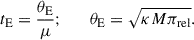
Thus, for events characterized by a short timescale with tE ≲ 6.3 days and a small angular Einstein radius with θE ≲ 0.12 mas, the lens is likely to be a BD with a mass below the hydrogen-burning limit.
In single-lens events, the event timescale is usually the only observable that can be derived from the light curve analysis. In such cases, a short timescale may be attributed to a high relative proper motion between the lens and source, rather than indicating a low-mass lens. Consequently, it is difficult to conclusively infer that the lens mass lies in the substellar regime based solely on tE. Although microlensing is a powerful tool for detecting BDs, it remains challenging to identify reliable BD candidates from single-lens events1.
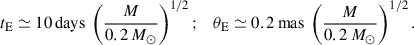
In binary-lens events involving two lens components, the probability of measuring the additional observable θE is high, as a significant fraction these events exhibit caustic-crossing features in their light curves. When both observables, tE and θE, are measured and found to be small, the likelihood that the lens has a low mass increases significantly. The event timescale and angular Einstein radius corresponding to each lens component is related to the mass ratio, q, between the components by the following relations:
 (3)
(3)
for the event timescale and
 (4)
(4)
for the angular Einstein radius. Here tE and θE are the values corresponding to the total mass of the binary lens system. If the binary lens consists of roughly equal-mass components, then events with tE ≲ 9 days and θE ≲ 0.17 mas suggest that each component is likely a BD with substellar mass.
An alternative approach to identifying BD events in binary-lens systems focuses on microlensing events with low-mass ratios between the lens components. This method is motivated by the fact that typical Galactic microlensing events are primarily caused by low-mass stars (Han & Gould 2003), and companions with low-mass ratios are likely to be BDs. By applying a selection criterion of q ≲ 0.1 to binary-lens events identified in microlensing survey data, dozens of BD candidates have been reported in previous studies (Han et al. 2022, 2023a,b, 2024). In these cases, only one component of the binary lens is inferred to be a BD.
Brown dwarfs are often described as “failed stars”, because they are too massive to be considered planets but not massive enough to sustain hydrogen fusion in the same way as ordinary stars. Because their physical properties place them in this in-between regime, their formation pathways remain uncertain.
The identification of binary BDs is valuable because the frequency, separation, and mass ratios of such systems provide important clues regarding whether they form in a stellar-like manner, through cloud fragmentation (Bate et al. 2002), or in a planet-like manner, through disk instability or core accretion (Whitworth & Goodwin 2005).
The microlensing method is particularly powerful in this context because it can reveal systems that are extremely faint, cold, and inaccessible to direct imaging. Moreover, microlensing surveys detect hundreds of lensing events caused by binary systems annually, with a significant fraction arising from binaries composed of BDs. The resulting datasets can provide valuable constraints on how common such binaries are in our galaxy and help in testing competing formation theories.
In this study, we examine microlensing data from the 2023 and 2024 observing seasons to search for events generated by binary systems composed of BDs. Our selection criteria require that both key lensing parameters, tE and θE, are securely measured and lie below defined threshold values. Based on these criteria, we identified six candidate binary-lens events in which both components are likely BDs.
2. Selection of candidate events and data
To identify binary BD candidates, we first examined binary-lens events detected from the Korea Microlensing Telescope Network (KMTNet; Kim et al. 2016) survey during the 2023 and 2024 seasons. The primary selection criterion was that the event exhibits well-resolved caustic features, ensuring that the angular Einstein radius can be securely measured. Additionally, we applied the criteria of tE ≲ 9 days and θE ≲ 0.17 mas. Using these criteria, we identified six candidate events: KMT-2023-BLG-1819, KMT-2023-BLG-2019, KMT-2024-BLG-1005, KMT-2024-BLG-1518, KMT-2024-BLG-2185, and KMT-2024-BLG-2486.
All of these events, with the exception of KMT-2023-BLG-2019, were also observed by other lensing surveys conducted by the Optical Gravitational Lensing Experiment (OGLE; Udalski et al. 2015) and the Microlensing Observations in Astrophysics (MOA; Bond et al. 2001; Sumi et al. 2003) collaborations. In Table 1, we provide a summary of the event correspondences, along with the equatorial and Galactic coordinates for each event, as well as the dates when alerts were issued by the individual survey groups. Among the events, four (KMT-2023-BLG-2019, KMT-2024-BLG-1005, KMT-2024-BLG-1518, and KMT-2024-BLG-2486) were initially identified by the KMTNet group, while two (MOA-2023-BLG-331 and MOA-2024-BLG-181) were first detected by the MOA group. For events observed by multiple surveys, we use the event ID assigned by the first detecting group as the representative designation, following the convention in the microlensing community.
Event correspondence, alert dates, and coordinates.
Photometric data for the events were obtained from observations conducted by the individual surveys. The KMTNet survey employs three identical telescopes, strategically located in the Southern Hemisphere for continuous coverage of lensing events: at Siding Spring Observatory in Australia (KMTA), Cerro Tololo Interamerican Observatory in Chile (KMTC), and South African Astronomical Observatory in South Africa (KMTS). Each KMTNet telescope has a 1.6 meter aperture and is equipped with a camera that provides a four square degree field of view. The MOA survey uses a 1.8 meter telescope situated at Mt. John University Observatory in New Zealand, with a camera that covers a 2.2 square degree field of view. The OGLE survey is conducted using the 1.3 meter Warsaw Telescope, located at Las Campanas Observatory in Chile. The camera mounted on the OGLE telescope has a field of view of 1.4 square degrees. Observations from the KMTNet and OGLE surveys were primarily carried out in the I band, whereas the MOA survey observations were made in a customized MOA-R band, with a wavelength range of 609 to 1109 nm.
The data used in the analyses were obtained by performing photometry with the pipelines developed by the respective survey groups: Albrow et al. (2009) for KMTNet, Bond et al. (2001) for MOA, and Udalski (2003) for OGLE. To correct the photometric uncertainties provided by the automated pipeline, we applied a rescaling procedure. The goal was to bring the reported error bars into agreement with the actual scatter in the measurements, and to adjust them such that the reduced χ2 of the model evaluation approached unity for each individual dataset. This adjustment followed the approach described by Yee et al. (2012).
In the case of KMTNet data, short-duration correlated noise may arise from residual images of previous exposures. Although microlensing light curves may exhibit diverse distortions, they rarely reproduce noise patterns found in observational data. On the rare occasions when a model reproduces very short-duration features, we inspected the images at the corresponding epochs to assess whether the signal is genuine. For the analyzed events, no such cases were identified.
3. Modeling light curves
Given the caustic-crossing features in all the analyzed events, we modeled the light curves using the binary-lens single-source (2L1S) configuration. In this model, the light curve is described by seven parameters. Three of these parameters (t0, u0, tE) represent the lens-source approach, with t0 denoting the time of closest approach, u0 indicating the separation at that time, and tE representing the event timescale. Two additional parameters (s, q) characterize the binary lens, where s is the projected separation between the lens components (M1 and M2) and q is their mass ratio. The parameters u0 and s are scaled to the angular Einstein radius corresponding to the total mass of the binary lens. The parameter α defines the direction of the source’s motion relative to the M1–M2 axis. The final parameter, ρ, represents the ratio of the angular source radius (θ*) to the angular Einstein radius, ρ = θ*/θE. This parameter (normalized source radius) accounts for finite-source effects, particularly in the caustic-crossing regions. Since all the lensing events have short durations, we do not consider long-term higher-order effects, such as the parallax effect from Earth’s orbital motion around the Sun (Gould 1992, 2000a) or the lens-orbital effect from the binary lens (Alcock et al. 2000; Bennett et al. 1999; Albrow et al. 2000).
In the modeling process, we searched for the set of lensing parameters (lensing solution) that best reproduces the observed light curve. In the initial stage, we grouped the parameters into two categories: (s, q) in one group and the remaining parameters in the other. We performed a grid search over the (s, q) parameter space, while the remaining parameters were optimized using a downhill method based on the Markov chain Monte Carlo (MCMC) technique. This first modeling stage yielded a χ2 map across the grid space, from which we identified local solutions. In the second stage, each of these local solutions was refined by allowing all parameters to vary freely. In cases for which multiple solutions provided comparably good fits to the data, we present all degenerate solutions. However, for all events analyzed in this study, a unique solution was found. In the following subsections, we detail the analysis for each individual event.
3.1. MOA-2023-BLG-331
The lensing event MOA-2023-BLG-331 was first detected by the MOA survey on July 24, 2023, corresponding to the abridged Heliocentric Julian date HJD′≡HJD − 2460000 = 150, and was later identified by the KMTNet and OGLE surveys the following day. The source is located in the overlapping region between the KMTNet prime fields BLG03 and BLG43, with observations conducted at a 30 minute cadence for each field, and a 15 minute cadence for combined observations. The baseline I-band magnitude of the source was Ibase = 20.03, and the extinction toward the field was AI = 1.05.
The lensing light curve for MOA-2023-BLG-331 is shown in Figure 1. Although the primary magnification occurred within a span of less than 10 days, the light curve was well-covered by dense data, revealing intricate anomaly features. The two spikes at HJD′∼149.4 and 151.8, along with the U-shaped region between them, indicate that these features are due to caustic crossings of the source. The bumps around HJD′∼148.3 and 153.5 appear to be caused by the source’s approach to the cusps of a binary caustic.
From a 2L1S modeling, we found a unique solution that explains all the anomalous features. The model curve is overlaid on the data points in Figure 1, and the corresponding model parameters are summarized in Table 2. The binary lens parameters, (s, q)∼(1.33, 1.55), suggest that the lens is a binary system with components of similar masses and a projected separation slightly larger than the Einstein radius. We note that a mass ratio greater than unity indicates that the source trajectory lay closer to the lower-mass component of the binary lens system. The estimated event timescale, tE = (6.418 ± 0.050) days, is relatively short. The timescales corresponding to the individual lens components are tE, 1 ∼ 4.0 days and tE, 2 ∼ 5.0 days, suggesting that both components are of low mass. The normalized source radius, ρ = (5.894 ± 0.051)×10−3, is measured with high precision due to the dense coverage of the caustic crossings. As we discuss in Section 4, the source is a main-sequence star. In lensing events involving an M-dwarf lens and a main-sequence source, the normalized source radius is typically ρ ≲ 2 × 10⁻³. Given that the angular Einstein radius is determined by θE = θ*/ρ, where θ* is the angular source radius, a measured ρ value significantly larger than the typical range implies that the angular Einstein radius is likely small.
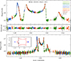 |
Fig. 1. Light curve of the lensing event MOA-2023-BLG-331. The bottom panel displays the full light curve, while the upper panels provide a zoomed-in view around the anomaly features and the residuals from the model. The curve overlaid on the data points represents the best-fit model. The inset in the bottom panel illustrates the lens system configuration, with the red cusped shape representing the caustic, the two blue dots indicating the positions of the lens components (with the larger dot representing the heavier lens component), and the arrowed line depicting the source’s trajectory. |
Lensing solutions of MOA-2023-BLG-331, KMT-2023-BLG-2019, and KMT-2024-BLG-1005.
The inset in the bottom panel of Figure 1 illustrates the configuration of the lens system. The binary lens created a resonant caustic structure featuring six cusps. The source star passed through the left side of the caustic, near the lower component of the lens, at an angle close to perpendicular. It first crossed the tip of the lower-left cusp, producing the initial bump in the light curve. It then entered and exited the left section of the caustic, resulting in a pair of sharp caustic spikes. After exiting, the source approached the upper-left cusp, giving rise to the final bump.
3.2. KMT-2023-BLG-2019
The lensing event KMT-2023-BLG-2019 was observed exclusively by the KMTNet survey. The source star lies in the overlapping region of two KMTNet prime fields, BLG01 and BLG41, both monitored at a high cadence of 30 minutes, providing dense temporal coverage of the light curve. The source had a baseline I-band magnitude of Ibase = 20.4, with an extinction of AI = 2.65 toward the field. The event was first identified on August 17, 2023 (corresponding to HJD′ = 173), after the light curve exhibited clear anomalies caused by caustic crossings.
Figure 2 presents the lensing light curve of KMT-2023-BLG-2019, which is marked by a pair of prominent caustic-crossing spikes occurring at HJD′∼170.4 and ∼172.3. Both caustic features were densely resolved, with each spike covered by the KMTS observations. In addition to these features, the light curve exhibits a weak bump around HJD′∼177. As with the previous event, the overall duration of the event is short, with the primary magnification phase concluding in under 10 days.
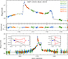 |
Fig. 2. Lensing light curve of KMT-2023-BLG-2019. The notations are the same as those used in Fig. 1. In the bottom panel, the left inset displays the full view of the caustic, while the right inset provides a close-up of the region where the source enters the caustic. |
A 2L1S modeling provides a unique solution that accounts for all the observed anomalous features. In Figure 2, we show the model curve superimposed on the data points. The complete set of lensing parameters is listed in Table 2. The derived binary parameters, (s, q)∼(1.53, 0.33), indicate that the lens is a binary system with components of comparable masses, separated by slightly more than the angular Einstein radius. As expected from the brief lensing magnification episode, the event timescale is relatively short, with tE = (6.328 ± 0.088) days. The individual timescales for the lens components are tE, 1 ∼ 5.4 days and tE, 2 ∼ 3.1 days. The well-resolved caustic features allowed for a precise measurement of the normalized source radius, ρ = (11.6 ± 0.22)×10−3. Given that the source is a main-sequence star, the unusually large value of ρ implies a small angular Einstein radius. Together with the short event timescales, this suggests that the lens has a low mass.
The configuration of the lens system is shown in the insets of the bottom panel, revealing a six-sided resonant caustic elongated along the binary axis. The source trajectory passed near the more massive lens component, first crossing the upper-left fold and then the lower fold of the caustic. These crossings account for the observed caustic-crossing features in the light curve. After exiting the caustic, the source passed near the lower-left cusp, which produced the weak bump observed in the light curve.
3.3. KMT-2024-BLG-1005
The lensing event KMT-2024-BLG-1005 involved a source with a baseline magnitude of Ibase = 19.2. It was first detected by the KMTNet group on May 16, 2024, and later confirmed by the OGLE group. The source is located within the region covered by the KMTNet prime fields BLG03 and BLG43, which were observed with a combined cadence of 15 minutes. The extinction in this field is AI = 1.24.
Figure 3 presents the light curve of the event, which, as with previous cases, is characterized by a short duration, with the main magnification phase lasting less than 10 days. The light curve features two distinct and well-defined caustic spikes occurring at approximately HJD′∼445.3 and HJD′∼448.3. Notably, the region between these two caustic spikes does not follow the typical U-shaped pattern commonly seen in caustic-crossing binary-lens events. Instead, it displays a relatively flat, plateau-like structure, indicating a deviation from the standard morphology. Both caustic features were clearly resolved, owing to the dense and continuous observational coverage provided by the combined data from the KMTA and KMTS observatories.
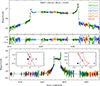 |
Fig. 3. Lensing light curve and lens-system configuration of KMT-2024-BLG-1005. |
We modeled the light curve using a 2L1S configuration and found a unique solution that explains the anomalous features. The binary-lens parameters, (s, q)∼(0.95, 0.36), suggest that the lens consists of two objects with comparable masses and a projected separation near the Einstein radius. The event timescale is tE = (3.593 ± 0.021) days, which is even shorter than those of the previous two events. The timescales corresponding to the individual lens components are tE, 1 ∼ 3.1 days and tE, 2 ∼ 1.8 days. From the analysis of the resolved caustics, we determined the normalized source radius to be ρ = (9.32 ± 0.17)×10−3. Given that the source is a main-sequence star, this relatively large ρ value suggests a small angular Einstein radius. Combined with the short event timescale, this implies that the lens is likely a low-mass object. The complete set of lensing parameters is provided in Table 2, and the corresponding model curve is shown in Figure 3.
The insets in the bottom panel of Figure 3 displays the lens-system configuration. Because of the binary separation being close to unity, the lens forms a resonant caustic with six cusps, elongated in the direction perpendicular to the binary axis. The source traversed the caustic diagonally, entering through the upper fold and exiting through the lower-right fold. These fold crossings generated the observed caustic spikes. The region between the spikes deviates from a typical U-shaped profile because, after entering the caustic, the source asymptotically approached the upper-left fold.
3.4. KMT-2024-BLG-1518
The lensing event KMT-2024-BLG-1518, which occurred on a source with a baseline magnitude of Ibase = 18.0, was observed by both the KMTNet and OGLE surveys. The KMTNet survey initially detected the event on June 25, 2024 (HJD′ = 486), shortly after the light curve exhibited a sharp brightening from the first caustic crossing. The OGLE survey identified the event four days later, on June 29, 2024 (HJD′ = 490), when the source experienced a second sharp rise due to another caustic crossing. The source is located in the KMTNet prime field BLG03, which mostly overlaps with BLG43, though the source lies in a non-overlapping region. As a result, KMTNet observations were conducted with a 30 minute cadence. The I-band extinction in this field is AI = 1.29.
The lensing light curve of KMT-2024-BLG-1518 is shown in Figure 4. It features two prominent caustic spikes at HJD′ = 484.5 and 486.6. The first caustic crossing was captured by the KMTS dataset, while the second was resolved through combined observations from OGLE, KMTC, and KMTS. Outside of these spikes, the source flux shows a smooth rise and fall, with no additional features. However, the region between the caustic spikes deviates from the typical U-shaped pattern, appearing asymmetric with a central portion that exhibits an approximately linear decline. The entire lensing magnification episode was completed within a span of less than 10 days.
Analysis of the light curve reveals that the event is well described by a unique 2L1S model. The best-fit binary-lens parameters are (s, q)∼(0.82, 0.90), indicating a binary lens composed of two nearly equal-mass objects with a projected separation slightly smaller than the Einstein radius. The full set of lensing parameters is provided in Table 3, and the corresponding model curve is shown in Figure 4. The event timescale is measured as tE = 5.118 ± 0.076 days, with individual timescales of tE, 1 ∼ 3.7 days and tE, 2 ∼ 3.5 days for the primary and secondary components, respectively. A detailed examination of the caustic-crossing features yields a normalized source radius of ρ = (8.60 ± 0.11)×10−3. Given that the source is identified as a main-sequence star, this relatively large ρ value is unusual for stellar-lens events with similar sources and suggests a small angular Einstein radius. The combination of the small θE and the short event timescale indicates that the lens is likely composed of low-mass objects.
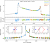 |
Fig. 4. Lensing light curve and lens-system configuration of KMT-2024-BLG-1518. |
Lensing solutions of KMT-2024-BLG-1518, MOA-2024-BLG-181, and KMT-2024-BLG-2486.
The insets in the bottom panel of Figure 4 illustrate the configuration of the lens system. The source traversed the central region of the caustic, entering through the lower-left fold located near the higher-mass lens component and exiting through the upper-right fold. As the source traversed the caustic, its trajectory closely followed the upper-left fold, resulting in an intra-caustic light curve that deviates from the typical U-shaped profile.
3.5. MOA-2024-BLG-181
The lensing magnification of MOA-2024-BLG-181 was first detected by the MOA group on August 9, 2024 (corresponding to HJD′ = 531), during the rising phase of the event. This detection was subsequently confirmed by the OGLE and KMTNet surveys. The source star was very faint, with a baseline magnitude of Ibase = 20.1, and the line of sight toward the field experienced an extinction of AI = 1.26. The event occurred in a region covered by both KMTNet prime fields BLG02 and BLG42, enabling observations at a high cadence of one data point every 15 minutes.
Figure 5 presents the lensing light curve of MOA-2024-BLG-181, which exhibits three notable features: a caustic spike at HJD′ = 532.2, a prominent bump centered around HJD′ = 532.8, and a weaker bump near HJD′ = 520.0. The spike caused by the source exiting the caustic was well resolved in the combined MOA and KMTA datasets, while the caustic entry spike was not observed but is estimated to have occurred around HJD′ = 531.3 based on an extrapolation of the U-shaped intra-caustic feature. The two bumps are likely due to the source passing near caustic cusps. The event was short, with the main magnification episode lasting less than 10 days.
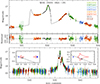 |
Fig. 5. Lensing light curve and lens-system configuration of MOA-2024-BLG-181. |
Modeling of the light curve yields a unique solution with binary-lens parameters of (s, q)∼(2.2, 1.7). The corresponding model curve is shown in Figure 5, and the full set of lensing parameters is listed in Table 3. The event timescale is measured as tE = 6.660 ± 0.049 days, indicating a short-duration event. The estimated Einstein timescales for the two lens components are approximately tE, 1 ∼ 4.0 days for M1 (the component closer to the source trajectory) and tE, 2 ∼ 5.3 days for M2 (the farther component). Analysis of the caustic-crossing features yields a precise measurement of the normalized source radius as ρ = (6.16 ± 0.12)×10−3. As with the previous events, this value is considerably larger than typical for main-sequence sources, suggesting a small angular Einstein radius.
The configuration of the lens system is shown in the insets of the bottom panel of Figure 5. Because the binary separation, s ∼ 2.2, is substantially larger than the Einstein radius, the caustic is divided into two segments (composed of four folds) located near each of the individual lens components. The source crossed the caustic near the lower-mass lens component (M1), producing the observed caustic spikes. After exiting the caustic, the source approached the on-axis cusp on the left side, resulting in the strong bump observed after the caustic spikes. The bump before the spikes was generated as the source passed near the heavier lens component (M2), but this bump is weak because the source approached the caustic at a relatively large distance.
3.6. KMT-2024-BLG-2486
The lensing event KMT-2024-BLG-2486 was observed by both the KMTNet and OGLE groups. The KMTNet group detected the event at a very early stage on September 9, 2024 (HJD′ = 531), and the OGLE group confirmed the event three days later. The source has a baseline magnitude of Ibase = 19.6, and the extinction toward the field is AI = 2.19. The source lay in the KMTNet prime fields BLG02 and BLG42, and the event was monitored with a 15 minute cadence.
The lensing light curve of the event is shown in Figure 6. It exhibits features similar to those of MOA-2024-BLG-181, characterized by a pair of caustic spikes at HJD′ = 561.1 and 561.4, with bumps appearing before and after the spikes. The pre-spike bump is centered around HJD′ = 540.0, while the post-spike bump, although only partially covered, is estimated to be centered around HJD′ = 562.0. In addition to the similarity in their anomaly features, both events also share the common trait of having short timescales.
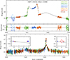 |
Fig. 6. Lensing light curve and lens-system configuration of KMT-2024-BLG-2486. |
Source color, magnitudes, and angular radius.
Motivated by the similarity of the anomaly pattern to that of MOA-2024-BLG-181, we performed a 2L1S modeling analysis, which yielded a unique solution with binary parameters (s, q)∼(3.0, 1.02). This indicates that the lens system comprises two nearly equal-mass components separated by approximately three times the Einstein radius in projection. The event timescale was measured to be tE = 7.395 ± 0.047 days, which is relatively short. The timescales corresponding to the individual lens components are estimated to be tE, 1 ∼ 5.2 days and tE, 2 ∼ 5.3 days, respectively. In addition, the normalized source radius was determined to be ρ = (5.231 ± 0.096)×10−3, a value substantially larger than what is typically found in events involving M-dwarf lenses with main-sequence source stars. This suggests that the Einstein ring of the lens system is relatively small. The model curve corresponding to the solution is superposed on the data points in Figure 6, and the full set of lensing parameters is listed in Table 3.
The configuration of the lens system is depicted in the insets of the bottom panel in Figure 6. Consistent with the similarity in the anomaly pattern, the lens configuration closely resembles that of MOA-2024-BLG-181. The binary lens creates two sets of four-fold caustics near the individual lens components, and the source passes through one of these caustics. The source path through the caustic is also similar: the source approach to M2 at a relatively large distance produced the weak post-spike bump, while the source approach to the on-axis cusp of the caustic near M1 led to the stronger post-spike bump.
4. Source stars and angular Einstein radii
Since the angular Einstein radius is obtained from the normalized source radius using the relation
 (5)
(5)
estimating θE requires knowledge of the angular size of the source star. This angular size was determined from the source’s color and magnitude after correcting for extinction and reddening. The source color and magnitude are also crucial for characterizing the source star itself.
The first step in characterizing a source star involves estimating its instrumental color, (V − I)S, and magnitude, IS. To determine the source magnitudes in the I and V bands, we began by generating light curves from the respective I- and V-band data, which were analyzed using the pyDIA photometry code (Albrow 2017). The source flux was then estimated by fitting each light curve with a model, A(t), according to the relation
 (6)
(6)
where Fobs(t) is the observed flux at time t, and (FS, Fb) represent the fluxes from the source and blended stars, respectively. Figure 7 displays the source positions on the instrumental color-magnitude diagrams (CMDs) of stars located near the event sources. The CMDs were constructed by performing photometry on neighboring stars in a consistent manner using the pyDIA code.
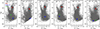 |
Fig. 7. Source positions of events in the instrumental color-magnitude diagrams. In each panel, the blue and red dots represent the positions of the source and the centroid of the red giant clump (RGC), respectively. For events with measured blended flux, the locations of the blends are also indicated by green dots. |
In the second step, the source color and magnitude were calibrated by correcting for extinction and reddening. This calibration was carried out using a reference with well-established de-reddened color and magnitude values. Specifically, we adopted the centroid of the red giant clump (RGC), whose de-reddened color, (V − I)RGC, 0, and magnitude, IRGC, 0, were previously determined by Bensby et al. (2013) and Nataf et al. (2013), respectively. By measuring the offset, Δ(V − I, I), between the source and the RGC centroid in the instrumental CMD, we determined the de-reddened source color and magnitude as
 (7)
(7)
Table 4 presents the instrumental color and magnitude of the source, (V − I, I)s, and those of the RGC centroid, (V − I, I)RGC, along with their corresponding de-reddened values, (V − I, I)s, 0 and (V − I, I)RGC, 0. The resulting source properties indicate that all sources are main-sequence dwarfs: the sources of KMT-2024-BLG-1518 and KMT-2024-BLG-2486 are G-type dwarfs, while the others are K-type dwarfs.
In the third step, we estimated the angular radius of the source star using the de-reddened color and magnitude derived earlier. Specifically, we applied the (V − K, I)–θ* relation from Kervella et al. (2004). To use this relation, the measured V − I color was first converted to V − K using the color–color transformation of Bessell & Brett (1988), and the angular source radius was then inferred from the (V − K, I)–θ* relation. The resulting angular source radii are listed in Table 4.
In the final step, the angular Einstein radius was estimated from the angular source radius using the relation given in Eq. (5). By combining the estimated angular Einstein radius with the event timescale, the relative lens-source proper motion was calculated as μ = θE/tE. The resulting values of θE and μ for the events are presented in Table 5. For all events, the estimated θE values are less than 0.2 mas. These small values, together with the short timescales, suggest that the lens masses are likely to be low.
Angular Einstein radii.
5. Probability of BD pair
We estimated the masses of the lens components to assess the likelihood that the lens is a binary composed of BDs. To accomplish this, we conducted a Bayesian analysis that incorporated constraints from the measured lensing observables, tE and θE, along with priors derived from a Galaxy model and the mass function of lens objects. The mass function characterizes the distribution of lens masses, while the Galaxy model defines the physical and dynamical distributions of the lenses.
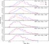 |
Fig. 8. Bayesian posteriors for the lens mass. The blue and red curves represent the posterior distributions of M1 and M2, respectively, where M1 denotes the lens component located closer to the source trajectory. |
In the Bayesian analysis, we began by generating a large number of artificial events using a Monte Carlo simulation. For each simulated lensing event, the physical parameters (M, DL, DS, μ)i were assigned based on a model mass function and Galaxy model. Specifically, we adopted the mass function from Jung et al. (2022) and the Galaxy model from Jung et al. (2021). The mass function was constructed by adopting the initial mass function for the bulge population, and the present-day mass function of Chabrier (2003) for the disk population. We considered remnant lenses, such as white dwarfs, neutron stars, and black holes, by adopting the Gould (2000b) model. In the Galaxy model, the bulge mass distribution is constructed by combining the Han & Gould (2003) model for the bulge, in which the bulge is modeled as a triaxial bar-shaped bulge with parameters derived from infrared star counts, and the modified double-exponential model of Bennett et al. (2014) for the disk. The velocity distribution of for bulge stars is constructed based on stars in the Gaia catalog (Gaia Collaboration 2016, 2018), while the distribution of disk stars follows a Gaussian form of Han & Gould (1995), and modified to adjust the Bennett et al. (2014) disk model.
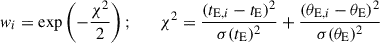
Using these parameters obtained from the Monte Carlo simulation, we calculated the corresponding lensing observables (tE, θE)i using the relations given in Eq. (1). Finally, the posteriors for the lens mass and distance were constructed by assigning a weight to each artificial event of
 (8)
(8)
Here (tE, θE) are the measured values of the lensing observables, and σ(tE) and σ(θE) represent their respective uncertainties.
In lensing analyses, among the two observables, tE is directly determined through light curve modeling, whereas the estimate of θE is independently derived from the source’s physical properties, specifically the angular radius θ* inferred from its color and brightness. Although θE = θ*/ρ, and a correlation between tE and ρ may exist such that tE and θE cannot be regarded as completely uncorrelated, in the present analysis θE is obtained through a separate procedure. Therefore, in practice this correlation is expected to be weak, since θE relies on independent estimates of the source’s angular radius.
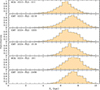 |
Fig. 9. Bayesian posteriors for the distance to the lens. |
Figures 8 and 9 show the posterior distributions for the mass and distance of the lenses for each individual event, obtained from the Bayesian analyses. The mass posterior distributions are presented separately for the binary lens components M1 and M2, with M1 referring to the lens component that is closer to the source trajectory. Table 6 provides the estimated physical parameters of M1, M2, DL, and a⊥, where a⊥ represents the projected physical separation between the lens components. For each lens parameter, the median of the posterior distribution is chosen as the central value, and the 16% and 84% percentiles are used to define the lower and upper bounds, respectively.
Physical lens parameters.
The values of pBD for M1 and M2 listed in Table 7 indicate the probabilities that the lens components lie within the BD mass range of 0.01 ≲ M/M⊙ ≲ 0.08. For the events KMT-2024-BLG-1005, KMT-2024-BLG-1518, MOA-2024-BLG-181, and KMT-2024-BLG-2486, the probabilities that both components of the binary lens fall within the BD mass range are greater than 50%, suggesting that these lenses are very likely binary BDs. In contrast, for MOA-2023-BLG-331L and KMT-2023-BLG-2019L, the probabilities that the lower-mass components of the binary lenses fall within the BD mass range exceed 50%, whereas the probabilities for the heavier components are below 50%. This implies that these systems are more likely to consist of a low-mass M dwarf and a BD.
Probabilities of being in the BD mass range, disk, and bulge.
It has been determined that the lenses for all events are likely located in the Galactic bulge. The values pdisk and pbulge in Table 7 represent the probabilities of the lenses being in the disk and bulge, respectively. For all events, the probability of the lens being in the bulge (pbulge) is significantly higher than that of being in the disk (pdisk). This is also reflected in the posterior distributions of DL.
6. Summary and discussion
With the goal of identifying binary-lens microlensing events in which both lens components have substellar masses, we examined binary-lens events detected in the 2023 and 2024 microlensing survey seasons. To identify potential binary BD candidates, we applied selection criteria that required short event timescales (tE ≲ 9 days) and small angular Einstein radii (θE ≲ 0.17 mas), both of which are indicative of low-mass lenses. An additional requirement was that the event display well-resolved caustic features, which are crucial for accurately measuring the angular Einstein radius. Through this selection process, we identified six candidate events likely to involve binary BD systems: MOA-2023-BLG-331, KMT-2023-BLG-2019, KMT-2024-BLG-1005, KMT-2024-BLG-1518, MOA-2024-BLG-181, and KMT-2024-BLG-2486.
Analysis of these events led to models that provided precise estimates for both lensing observables, tE and θE. Utilizing the constraints provided by these observables, we estimated the masses of the binary components through Bayesian analysis. The analysis indicated that in the cases of KMT-2024-BLG-1005, KMT-2024-BLG-1518, MOA-2024-BLG-181, and KMT-2024-BLG-2486, there is a greater than 50% chance that both components of the lens systems have substellar masses, strongly pointing to their nature as binary BDs. In contrast, MOA-2023-BLG-331L and KMT-2023-BLG-2019L suggest mixed-mass systems, where the secondary components have a high probability of being BDs, but the primary components are more likely low-mass M dwarfs, indicating these lenses are likely composed of an M dwarf–BD pair.
The BD nature of the binary components can be confirmed through future high-resolution imaging with instruments such as the European Extremely Large Telescope. If the more massive component (MA) of a binary lens is a star, it will become detectable once the source and lens are sufficiently separated. Therefore, if we wait until this separation occurs and still do not detect the lens, it would indicate that both components are BDs. Conversely, if the brighter lens component is detected, its mass can be measured, which in turn allows us to determine the mass of the secondary component and assess whether it falls within the BD regime.
To estimate the time required to resolve the lens and source, we first compute the K-band contrast ratio between them as
 (9)
(9)
where ΔAK = AK, S − AK, L is the difference in extinction between the source and lens. For all analyzed events, the lens distances are ≳6 kpc, so we adopt ΔAK ≈ 0. The K-band magnitude of the source, KS, 0, is estimated using the (V − I, I)S, 0 color and magnitude, together with the relation of Bessell & Brett (1988). The K-band magnitude of the lens is estimated as
 (10)
(10)
where the absolute magnitude is set to MK, L = 10, corresponding to a star with the minimum stellar mass M*, min = 0.08 M⊙ (Figure 22 of Benedict et al. 2016) which is the hydrogen-burning limit at the boundary between stars and BDs. The distance to the lens is given by DL = AU/(πrel + πS) kpc, where πrel = θE, A2/(8.14 M*, min) is the lens-source relative parallax (in mas), and πS = AU/(8.5 kpc)≈0.117 mas is the parallax of the source, assuming DS = 8.5 kpc. The angular Einstein radius corresponding to the primary mass MA = M*, min is θE, A = [1/(1 + q)]1/2θE.
Contrast ratio between the lens and source.
Table 8 lists the contrast ratios for the individual events, with ΔK0 values ranging from 6.7 to 8.2, corresponding to flux ratios between 500 and 2000. Due to this high contrast, resolving the lens from the source would require a separation of approximately 8–10 times the FWHM, which translates to about 110–140 mas. Assuming the lower limit of 110 mas, the lens and source could be resolved after a wait time of approximately 8 years (in 2032) for KMT-2024-BLG-1005, which has the highest proper motion of μ ∼ 13.3 mas/yr. For KMT-2024-BLG-2486, which has the lowest proper motion of μ ∼ 5.5 mas/yr, the required separation would be reached in about 20 years (in 2044).
Given that six candidates were identified in just two years of data, it is likely that additional BD binaries can be discovered in the full microlensing survey dataset. Furthermore, more precise mass measurements could, in principle, be obtained by measuring microlens parallax in events observed by future space-based missions such as the Nancy Grace Roman Space Telescope and the Chinese Space Station Telescope.
Under specific observational conditions, when a short timescale, high-magnification event is observed simultaneously from two sites, the lens mass can be uniquely determined by measuring the microlens parallax (πE) (Refsdal 1966; Gould 1994). This method was employed to identify three isolated BDs, OGLE-2007-BLG-224 (Gould et al. 2009), OGLE-2017-BLG-0896L (Shvartzvald et al. 2019), and OGLE-2017-BLG-1186L (Li et al. 2019), through the measurement of πE.
Acknowledgments
This research was supported by the Korea Astronomy and Space Science Institute under the R&D program (Project No. 2025-1-830-05) supervised by the Ministry of Science and ICT. This research has made use of the KMTNet system operated by the Korea Astronomy and Space Science Institute (KASI) at three host sites of CTIO in Chile, SAAO in South Africa, and SSO in Australia. Data transfer from the host site to KASI was supported by the Korea Research Environment Open NETwork (KREONET). C.Han acknowledge the support from the Korea Astronomy and Space Science Institute under the R&D program (Project No. 2025-1-830-05) supervised by the Ministry of Science and ICT. J.C.Y., I.G.S., and S.J.C. acknowledge support from NSF Grant No. AST-2108414. W.Zang acknowledges the support from the Harvard-Smithsonian Center for Astrophysics through the CfA Fellowship. The MOA project is supported by JSPS KAKENHI Grant Number JP16H06287, JP22H00153 and 23KK0060. C.R. was supported by the Research fellowship of the Alexander von Humboldt Foundation.
References
- Albrow, M. 2017, https://doi.org/10.5281/zenodo.268049 [Google Scholar]
- Albrow, M. D., Beaulieu, J.-P., Caldwell, J. A. R., et al. 2000, ApJ, 534, 894 [NASA ADS] [CrossRef] [Google Scholar]
- Albrow, M., Horne, K., Bramich, D. M., et al. 2009, MNRAS, 397, 2099 [Google Scholar]
- Alcock, C., Allsman, R. A., Alves, D., et al. 2000, ApJ, 541, 270 [NASA ADS] [CrossRef] [Google Scholar]
- Bate, M. R., Bonnell, I. A., & Bromm, V. 2002, MNRAS, 332, L65 [NASA ADS] [CrossRef] [Google Scholar]
- Benedict, G. F., Henry, T. J., Franz, O. G., et al. 2016, AJ, 152, 141 [Google Scholar]
- Bennett, D. P., Rhie, S. H., Becker, A. C., et al. 1999, Nature, 402, 57 [NASA ADS] [CrossRef] [Google Scholar]
- Bennett, D. P., Batista, V., Bond, I. A., et al. 2014, ApJ, 785, 155 [Google Scholar]
- Bensby, T., Yee, J. C., Feltzing, S., et al. 2013, A&A, 549, A147 [NASA ADS] [CrossRef] [EDP Sciences] [Google Scholar]
- Bessell, M. S., & Brett, J. M. 1988, PASP, 100, 1134 [Google Scholar]
- Bond, I. A., Abe, F., Dodd, R. J., et al. 2001, MNRAS, 327, 868 [Google Scholar]
- Chabrier, G. 2003, PASP, 115, 763 [Google Scholar]
- Gaia Collaboration (Prusti, T., et al.) 2016, A&A, 595, A1 [NASA ADS] [CrossRef] [EDP Sciences] [Google Scholar]
- Gaia Collaboration (Brown, A. G. A., et al.) 2018, A&A, 616, A1 [NASA ADS] [CrossRef] [EDP Sciences] [Google Scholar]
- Gould, A. 1992, ApJ, 392, 442 [Google Scholar]
- Gould, A. 1994, ApJ, 421, L71 [NASA ADS] [CrossRef] [Google Scholar]
- Gould, A. 2000a, ApJ, 535, 928 [Google Scholar]
- Gould, A. 2000b, ApJ, 542, 785 [NASA ADS] [CrossRef] [Google Scholar]
- Gould, A., Udalski, A., Monard, B., et al. 2009, ApJ, 698, L147 [Google Scholar]
- Han, C., & Gould, A. 1995, ApJ, 447, 53 [Google Scholar]
- Han, C., & Gould, A. 2003, ApJ, 592, 172 [Google Scholar]
- Han, C., Ryu, Y.-H., Shin, I.-G., Jung, Y. K., et al. 2022, A&A, 667, A64 [NASA ADS] [CrossRef] [EDP Sciences] [Google Scholar]
- Han, C., Jung, Y. K., Kim, D., et al. 2023a, A&A, 675, A71 [NASA ADS] [CrossRef] [EDP Sciences] [Google Scholar]
- Han, C., Jung, Y. K., Bond, I. A., et al. 2023b, A&A, 678, A190 [NASA ADS] [CrossRef] [EDP Sciences] [Google Scholar]
- Han, C., Bond, I. A., Udalski, A., et al. 2024, A&A, 691, A237 [NASA ADS] [CrossRef] [EDP Sciences] [Google Scholar]
- Jung, Y. K., Han, C., Udalski, A., et al. 2021, AJ, 161, 293 [NASA ADS] [CrossRef] [Google Scholar]
- Jung, Y. K., Zang, W., Han, C., et al. 2022, AJ, 164, 262 [NASA ADS] [CrossRef] [Google Scholar]
- Kervella, P., Thévenin, F., Di Folco, E., & Ségransan, D. 2004, A&A, 426, 29 [Google Scholar]
- Kim, S.-L., Lee, C.-U., Park, B.-G., et al. 2016, JKAS, 49, 37 [Google Scholar]
- Li, S.-S., Zang, W., Udalski, A., et al. 2019, MNRAS, 488, 3308 [NASA ADS] [CrossRef] [Google Scholar]
- Nataf, D. M., Gould, A., Fouqué, P., et al. 2013, ApJ, 769, 88 [Google Scholar]
- Refsdal, S. 1966, MNRAS, 134, 315 [NASA ADS] [CrossRef] [Google Scholar]
- Shvartzvald, Y., Yee, J. C., Skowron, J., et al. 2019, AJ, 157, 106 [NASA ADS] [CrossRef] [Google Scholar]
- Sumi, T., Abe, F., Bond, I. A., et al. 2003, ApJ, 591, 204 [NASA ADS] [CrossRef] [Google Scholar]
- Udalski, A. 2003, Acta Astron., 53, 291 [NASA ADS] [Google Scholar]
- Udalski, A., Szymański, M. K., & Szymański, G. 2015, Acta Astron., 65, 1 [NASA ADS] [Google Scholar]
- Whitworth, A. P., & Goodwin, S. P. 2005, Astron. Nachr., 326, 899 [Google Scholar]
- Yee, J. C., Shvartzvald, Y., Gal-Yam, A., et al. 2012, ApJ, 755, 102 [Google Scholar]
All Tables
Lensing solutions of MOA-2023-BLG-331, KMT-2023-BLG-2019, and KMT-2024-BLG-1005.
Lensing solutions of KMT-2024-BLG-1518, MOA-2024-BLG-181, and KMT-2024-BLG-2486.
All Figures
|
Fig. 1. Light curve of the lensing event MOA-2023-BLG-331. The bottom panel displays the full light curve, while the upper panels provide a zoomed-in view around the anomaly features and the residuals from the model. The curve overlaid on the data points represents the best-fit model. The inset in the bottom panel illustrates the lens system configuration, with the red cusped shape representing the caustic, the two blue dots indicating the positions of the lens components (with the larger dot representing the heavier lens component), and the arrowed line depicting the source’s trajectory. |
| In the text | |
|
Fig. 2. Lensing light curve of KMT-2023-BLG-2019. The notations are the same as those used in Fig. 1. In the bottom panel, the left inset displays the full view of the caustic, while the right inset provides a close-up of the region where the source enters the caustic. |
| In the text | |
|
Fig. 3. Lensing light curve and lens-system configuration of KMT-2024-BLG-1005. |
| In the text | |
|
Fig. 4. Lensing light curve and lens-system configuration of KMT-2024-BLG-1518. |
| In the text | |
|
Fig. 5. Lensing light curve and lens-system configuration of MOA-2024-BLG-181. |
| In the text | |
|
Fig. 6. Lensing light curve and lens-system configuration of KMT-2024-BLG-2486. |
| In the text | |
|
Fig. 7. Source positions of events in the instrumental color-magnitude diagrams. In each panel, the blue and red dots represent the positions of the source and the centroid of the red giant clump (RGC), respectively. For events with measured blended flux, the locations of the blends are also indicated by green dots. |
| In the text | |
|
Fig. 8. Bayesian posteriors for the lens mass. The blue and red curves represent the posterior distributions of M1 and M2, respectively, where M1 denotes the lens component located closer to the source trajectory. |
| In the text | |
|
Fig. 9. Bayesian posteriors for the distance to the lens. |
| In the text | |
Current usage metrics show cumulative count of Article Views (full-text article views including HTML views, PDF and ePub downloads, according to the available data) and Abstracts Views on Vision4Press platform.
Data correspond to usage on the plateform after 2015. The current usage metrics is available 48-96 hours after online publication and is updated daily on week days.
Initial download of the metrics may take a while.