| Issue |
A&A
Volume 704, December 2025
|
|
|---|---|---|
| Article Number | A43 | |
| Number of page(s) | 9 | |
| Section | Astronomical instrumentation | |
| DOI | https://doi.org/10.1051/0004-6361/202555737 | |
| Published online | 28 November 2025 | |
Non-convex sparse regularisation for radio interferometric imaging via smoothly clipped absolute deviation
1
School of Computer Science and Technology, Zhejiang Sci-Tech University,
Hangzhou
310018,
China
2
State Key Laboratory of Solar Activity and Space Weather, National Space Science Center, Chinese Academy of Sciences,
Beijing
100190,
China
3
Radio Science and Technology Center (π Center),
Chengdu
610041,
China
★ Corresponding author: This email address is being protected from spambots. You need JavaScript enabled to view it.
Received:
30
May
2025
Accepted:
27
October
2025
Abstract
Context. Reconstructing a high-resolution image of observed radio sources from the incomplete visibilities poses a challenging, ill-posed, inverse problem. Although compressive sensing has demonstrated remarkable performance in radio interferometric imaging, traditional compressed sensing methods approximately replace the L0-norm minimisation problem with the L1-norm minimisation problem, which brings about a bias issue.
Aims. To ameliorate the bias problem and efficiently obtain an accurate solution in radio interferometry, we propose a novel, non-convex sparse regularisation method based on smoothly clipped absolute deviation (SCAD) in this paper.
Methods. The proposed method utilises the continuous SCAD penalty function to approximate the L0 norm and efficiently solves the non-convex optimisation problem by using an improved proximal gradient algorithm. The improved proximal gradient algorithm introduces a restart strategy and an adaptive non-monotonic step-size strategy to improve the convergence speed of the algorithm. Moreover, the regularisation parameter was adaptively updated using the prior information of the image.
Results. Numerical simulation experiments are carried out on the Very Large Array (VLA) and Square Kilometre Array (SKA). We compare the proposed method with state-of-the-art imaging methods. The results show thatitperforms better in terms of reconstruction quality and computational efficiency.
Key words: instrumentation: interferometers / methods: numerical / techniques: image processing
© The Authors 2025
 Open Access article, published by EDP Sciences, under the terms of the Creative Commons Attribution License (https://creativecommons.org/licenses/by/4.0), which permits unrestricted use, distribution, and reproduction in any medium, provided the original work is properly cited.
This article is published in open access under the Subscribe to Open model. This email address is being protected from spambots. You need JavaScript enabled to view it. to support open access publication.
1 Introduction
Currently, radio interferometry has become an indispensable tool for astronomical observation, and it plays an important role in many fields of astronomy and astrophysics. It is well known that only part of the complete uv coverage can be measured by the interferometric array. The imaging process is a typical, ill-posed, linear inverse problem. Astronomers routinely employ the Hogbom CLEAN algorithm (Högbom 1974) along with its variants for radio interferometric imaging, such as multi-scale CLEAN (Cornwell 2008, 2009; Rich et al. 2008) and adaptive-scale CLEAN (Bhatnagar & Cornwell 2004; Zhang et al. 2016; Zhang 2018; Zhang et al. 2020). Although the CLEAN family effectively reduces side-lobe interference caused by incomplete uv coverage, the CLEAN family often produces sub-optimal imaging quality.
In recent years, the theory of compressed sensing (CS; Donoho 2006; Li et al. 2020) has provided a new solution for radio interferometric imaging. By utilizing the sparsity of the signal, CS can reconstruct high-quality images at low sampling rates. However, the L0 -norm optimisation problem in CS is non-deterministic polynomial time hard (NP-hard). Aiming to resolve this problem, researchers have proposed a variety of alternative methods to obtain sub-optimal solutions. Among them, the widely used method is convex optimisation for solving the L1-norm minimisation problem or reweighted L1-norm minimisation problem (Condat 2014; Bubeck et al. 2015; Xu & Noo 2022).
Based on convex optimisation techniques, many CS-based approaches have been developed in radio interferometric imaging, such as the isotropic undecimated wavelet transform (IUWT; Li et al. 2011; Garsden et al. 2015) and sparsity-averaging reweighted analysis (SARA; Carrillo et al. 2012, Carrillo et al. 2014; Onose et al. 2016, 2017; Dabbech et al. 2022; Terris et al. 2023; Wilber et al. 2023a). The IUWT algorithm adopts an isotropic undecimated wavelet basis as the sparse basis according to the characteristics of astronomical images and then solves the L1 -norm minimisation problem by the fast iterative shrinkagethresholding algorithm. Experimental results show that its reconstruction quality is superior to the Högbom-CLEAN and multiscale CLEAN algorithms. The SARA algorithm uses a dictionary composed of a Dirac basis and multiple wavelet bases as the sparse basis, and then solves the reweighted L1 -norm minimisation problem by a variety of fast and parallelisable algorithms, such as the primal-dual forward-backward (PDFB) one, the alternating direction method of multipliers (ADMM), and the preconditioned primal-dual (PPD; Onose et al. 2016, 2017) method. The simulation results have shown that the reconstruction quality of the SARA is superior to that of the total variation (TV) and IUWT algorithms (Carrillo et al. 2012). In view of the excellent performance of the SARA algorithm, researchers have extended it to the polarized imaging and wide-band imaging in radio interferometry, namely the Polarized SARA (Birdi et al. 2018, 2020) and HyperSARA algorithms (Abdulaziz et al. 2019; Thouvenin et al. 2023a,b).
In addition, with the rapid development of artificial-intelligence technology, researchers have begun to explore the use of deep neural networks (DNNs) for end-to-end reconstruction in radio interferometry (Gheller & Vazza 2022). Furthermore, an artificial intelligence for regularisation in radio-interferometric Imaging (AIRI) approach is presented (Wilber et al. 2023b; Terris et al. 2023), which simultaneously inherits the advantages of convex optimisation and deep learning. Recently, astronomers have proposed a residual-to-residual DNN series for a high-dynamic-range imaging (R2D2) algorithm (Dabbech et al. 2024; Aghabiglou et al. 2024), which adopts a DNN series architecture based on a residual-to-residual method. It uses a DNN to directly learn to generate updates from the current image estimate and the residual dirty image.
It is worth noting that traditional compressed sensing methods approximately replace the L0 norm by the L1 norm or weighted L1 norm, resulting in a bias problem. Specifically, the L0 norm only cares about whether an element is non-zero rather than its actual magnitude. However, the L1 norm punishes the elements based on their size. During the reconstruction process, small non-zero elements are easily compressed to zero, and the estimated values of large non-zero elements are also smaller than their actual values, resulting in a deviation between the reconstructed signal and the true sparse signal. Essentially, the bias stems from the compromise made in the accuracy of the sparsity measurement in order to achieve the solvability of the optimisation problem owing to the fact that convex optimisation has a global optimal solution (Zou & Hastie 2005; Candes et al. 2008; Jia et al. 2018).
To ameliorate the bias problem, Yang et al. (2025) proposed a Lq proximal gradient (LPG) algorithm with 0 < q < 1. However, the Lq norm (Marjanovic & Solo 2012) is still a biased approximation of the L0 norm, and the derivative of the Lq norm at the zero point does not exist. In contrast, the smoothly clipped absolute deviation (SCAD; Fan & Li 2001; Wen et al. 2018) has asymptotic unbiasedness under certain conditions. Moreover, it is continuously differentiable and can efficiently find the optimal solution in the optimisation process. To efficiently obtain an accurate solution in radio interferometry, we propose a non-convex, sparse regularisation method dubbed improved SCAD (ISCAD) in this paper. Our proposed approach employs the continuous SCAD penalty to approximate the L0 norm and leverages an improved proximal-gradient algorithm to effectively address the non-convex optimisation problem. Compared with the existing proximal gradient algorithms (Wen et al. 2018), the main improvements of the proposed algorithm lie in the following two aspects. On one hand, we adopted an adaptive, non-monotonic step-size (ANMS) strategy (Liu et al. 2022) to enhance the convergence rate of the proximal gradient algorithm for a non-convex optimisation problem. On the other hand, we adaptively updated the regularisation parameter using the prior information of the image.
The paper is structured as follows. Section 2 briefly introduces typical radio interferometric imaging methods based on CS. Section 3 describes a non-convex sparse regularisation method based on SCAD in detail. In Sect. 4, we describe several simulation experiments carried out to assess the performance of the proposed method. Section 5 provides the final conclusion.
2 Radio interferometric imaging methods based on compressed sensing
A radio interferometer generates the visibilities by measuring the correlation between the signals received by a pair of spatially separated antennas. Based on the Van Cittert–Zernike theorem (Thompson et al. 2017), under the simplifying assumptions of a coplanar array the relationship between the signal, x, and the measured visibilities, y, is given by
 (1)
(1)
where u = (u, v) represents the baseline vector normalised by the wavelength, l = (l, m) is the coordinate on the image plane, and A(l) is the primary beam that limits the observed field of view. After the discretisation of Eq. (1), a linear measurement model can be obtained as follows:
 (2)
(2)
where the vectors y ∈ CM and x ∈ RN stand for the visibilities and sampled intensity signal separately, n ∈ CM represents the noise vector, and the matrix Φ = GFZ ∈ CM×N represents the linear mapping from the image domain to the visibility domain. The matrix G ∈ CM×nN includes compact support interpolation kernels and models the direction-dependent effects (DDEs), F ∈ CnN×nN represents an n-oversampled discrete Fourier operator, and Z ∈ RnN×N denotes an oversampling and scaling operator for pre-compensated interpolation. It is unfortunate that Eq. (2) is an ill-posed inverse problem (Rau et al. 2009). At present, the CS technology has been successfully applied to radio interferometric imaging, and the state-of-the-art CS-based methods in radio interferometry are the SARA and AIRI.
According to CS theory, the signal, x, needs to be sparse or compressible on the orthogonal basis, ψ, namely x = ψα, where α denotes the decomposition of the signal on the sparse basis. While the measurement matrix satisfies the restricted isometry property (RIP; Candes et al. 2011; Shen & Hu 2019), the signal can be recovered by solving the following minimisation problem:
 (3)
(3)
where ||·||0 represents the L0 norm of the vector, α, and ε is the upper bound of the L2 norm of the noise vector. It should be noted that Eq. (3) is NP-hard and intractable.
The SARA algorithm proposed by Carrillo et al. (2012) adopts the concatenation of a Dirac basis and eight Daubechies wavelet bases (Db1-Db8) as a sparsity dictionary in radio interferometric imaging. With respect to a single sparse basis, the average of multiple sparse bases can promote the sparsity of the signal. And the SARA algorithm replaced Eq. (3) by the reweighted L1 minimisation problem; this is defined as
 (4)
(4)
where  denotes the reality and positivity prior on x, and W stands for the diagonal matrix with positive weights. In this work, PPD (Onose et al. 2017) was employed to solve Eq. (4).
Based on the unconstrained version of the SARA algorithm, namely uSARA, the AIRI algorithm (Terris et al. 2023) trains a DNN as the denoiser to replace the proximal operator in the regularisation step of the uSARA algorithm:
 (5)
(5)
where D refers to the DNN denoiser, γ is the step size, and ∇f is the gradient of the data-fidelity term  . Experimental results show that the AIRI algorithm outperforms the traditional SARA algorithm in terms of both reconstruction accuracy and speed (Wilber et al. 2023b).
We note that traditional CS algorithms generally approximate the NP-hard L0-norm minimisation problem by the L1-norm or reweighted one, which introduces certain deviations and affects the accuracy of the reconstruction results. In order to remedy the bias issue, Yang et al. (2025) proposed a radio-interferometric-imaging method based on Lq norm. The leastsquares problem with the Lq norm is given by
 (6)
(6)
where λ refers to the regularisation parameter,  stands for Lq norm, and the dictionary used in LPG is the same as that in SARA. Equation (6) is efficiently solved by the proximal gradient algorithm.
3 Non-convex, sparse regularisation based on smoothly clipped absolute deviation
Theleast-squares problem with the SCAD term can be expressed as
 (7)
(7)
where the dictionary ψ used is the same as that in SARA and LPG. Pλ(·) represents the SCAD penalty, which is defined as follows (Fan & Li 2001):
 (8)
(8)
where a > 2 is a constant and usually set to 3.7 (Fan & Li 2001). From Eq. (8), it can be seen that when the coefficient, z, is small, SCAD behaves similarly to the L1 norm, imposing strong penalties on small coefficients to make them zero. As the coefficient increases, SCAD takes on a smooth quadratic function form, avoiding excessive penalties for large coefficients. Figure 1 compares different penalty functions. It should be remarked that the Lq norm bridges the gap between the L0 norm and the L1 norm. Moreover, SCAD exhibits a closer approximation to the L0 norm than the Lq norm.
The proximal operator is of vital significance in developing efficient and scalable algorithms for numerous optimisation problems, especially for non-convex and non-smooth optimisation problems. For a penalty function, Pλ(·), the corresponding proximal mapping operator is given by
 (9)
(9)
For the SCAD penalty, the corresponding proximal operator is given by
 (10)
(10)
where sign(·) represents the sign function. For the sake of facilitating comparison, the penalty functions and the corresponding proximal operators of L0 norm, L1 norm, and Lq norm are listed in Table 1.
Figure 2 shows the outputs of proximal operators corresponding to different penalty functions. One can notice that the proximal operator of L0 norm is discontinuous, and the proximal operator of L1 norm is continuous but has deviations from that of L0 norm. The proximal operator of Lq norm is discontinuous and is less biased than that of the L1 norm. In contrast, the proximal operator of SCAD not only remains continuous, it also results in unbiased estimates of large coefficients.
To effectively address the non-convex optimisation problem, we adopt an improved proximal-gradient algorithm (Wen et al. 2018). The reconstructed image is given by
 (11)
(11)
where proxλ(·) stands for the proximal operator defined in Eq. (10), and the step size ακ+1 ∈ (0, 2/L) is generally a constant, where L is the Lipschitz constant of ∇f. s(k) denotes the temporary vector and is given by
 (12)
(12)
where  denotes the acceleration factor, and its initial value t(0) is usually set to one.
In addition, we adopted two strategies to accelerate the convergence speed of the algorithm. The first strategy is a gradientrestart one. It means that if  , the acceleration factor t(k+1) is reset to one, thereby eliminating oscillations (O’donoghue & Candes 2015).
Another strategy is an ANMS one. Liu et al. (2022) designed an ANMS strategy to increase the convergence rate of fast iterative shrinkage-thresholding algorithm (FISTA) for non-smooth and convex minimisation problems. In this paper, we applied the ANMS strategy to enhance the convergence rate of the proximal gradient algorithm for the non-convex optimisation problem. In the ANMS strategy, the acceleration factor is rewritten as
 (13)
(13)
where θ(k) = α(k)/α(k+1); the step size, α(k+1), is adaptively updated by


else
 (14)
(14)
where 〈·〉 represents the inner product, µ0, µ1 are two constants satisfying 0 <µ1 < µ0 < 1, and  is the control parameter with a constant w, which can be adjusted adaptively to control the growth amplitude of the step size.
The selection of the regularisation parameter, λ, is of vital importance to the performance of the algorithm. Generally, it is set based on experience and keeps constant during the iterative process. However, the empirical selection method poses challenges to achieving an optimal equilibrium between the data fidelity term and the regularisation term. To address this issue, this paper proposes an adaptive selection method, which makes full use of the information of the data fidelity term and the regularisation term to update the regularisation parameter (Yang et al. 2024). The regularisation parameter is updated by
 (15)
(15)
where the factor ζ is a constant.
Finally, the computational complexity of different algorithms was analysed. For the SARA algorithm solved by PPD, the computational complexity is O(nN log nN) + O(dN) + O(MN) per iteration, where n denotes the oversampling factor, and d denotes the number of blocks into which the visibility data is divided (Onose et al. 2017). For the LPG and ISCAD algorithms, the computational complexity is the same and is O(nN log nN) + O(N) per iteration. It can be seen that the computational complexity of the LPG and ISCAD algorithms per iteration is evidently lower than that of the SARA algorithm.
It should be noted that, with respective to convex optimisation, the specificities of the proposed algorithm mainly lie in the differences in the approximation accuracy of sparsity and the optimisation characteristics. Compared with convex optimisation, the proposed method utilises piecewise-designed SCAD penalty to be closer to the L0 norm, thereby reducing the bias problem. However, non-convex optimisation faces challenges such as local optima and low convergence efficiency. Therefore, the proposed method adopts restart and ANMS strategies to address these issues. From the perspective of application scope, the proposed algorithm is more suitable for handling high sparsity or structured sparse signals.
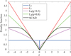 |
Fig. 1 Comparison of different penalty functions. |
Proximal operators for different penalty functions.
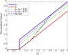 |
Fig. 2 Outputs of proximal operators corresponding to penalty functions. |
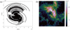 |
Fig. 3 (a) VLA baseline coverage. (b) Test image from 30Dor, presented on a log10 scale. |
4 Simulation results
We conducted numerical simulation experiments based on the Very Large Array (VLA; Perley et al. 2011) and Square Kilometre Array (SKA; Dewdney et al. 2009). We compared the performance of the proposed ISCAD method with respect to classical imaging methods such as the SARA1, AIRI2, and LPG3 methods. All programs were executed in the same hardware and software environment: MATLAB R2022a running on a personal computer equipped with the 2.5GHz Intel i9-12900H processor and 16 GB memory. In addition, we optimised and set the parameters of SARA, AIRI, and LPG according to Onose et al. (2017), Terris et al. (2023), and Yang et al. (2025). The DNN denoiser of AIRI in this article is the same as that trained on optical astronomy images in the Terris et al. (2023). In the LPG method, the value of q in the Lq norm is 0.8 (Yang et al. 2025). The main parameters of ISCAD are set as follows: α = 3.7, µ0 = 0.99, µ1 = 0.95, w = 1, ζ ∈ [10–6,10–3].
The signal-to-noise ratio (S/N) and S/Nlog were used to measure the reconstruction accuracy. They can be expressed as follows:
 (16)
(16)
 (17)
(17)
where x and  denote the original image and the reconstructed image separately, and ε refers to the estimated noise level, and IN is the unit vector with the length N.
In the simulations, we assumed a small field of view and the absence of DDEs such that the measurement operator reduces to a Fourier operator. We employed an oversampled Fourier transform, F, with n = 4 and a matrix, G, that interpolates frequency data to average a nearby uniformly distributed frequency via 8 × 8 Kaiser-Bessel interpolation kernels (Fessler & Sutton 2003).
In the initial experiment, We used the VLA baseline coverage generated by the CASA and CASACORE (Onose et al. 2016, 2017). Figure 3a depicts the VLA baseline coverage containing 894240 uv points. Meanwhile, Fig. 3b illustrates the test image with a pixel size of 256 × 256, presented on a log10 scale. This test image was derived from the 30 Doradus (30Dor)4 in the Large Magellanic Cloud, and has brightness temperature values spanning the interval [0.01, 1].
When the input S/N (iS/N) of the additive Gaussian noise is set at 35dB, Fig. 4 illustrates the reconstruction results obtained by the SARA, AIRI, LPG, and ISCAD algorithms, respectively. In Fig. 4, the left column exhibits the reconstructed images on a log10 scale. the middle column displays the error images  on a linear scale, while the right column represents the real part of the residual images also in a linear scale. An inspection of Fig. 4 reveals that the inversion result of SARA manifests large residual errors and distinct artefacts for both the cobweb-like structure and the background. In comparison to SARA, AIRI, and LPG yield more favourable inversion results, with a notable reduction in both errors and artifacts. Furthermore, ISCAD produces a reconstructed image characterised by scarcely perceptible errors and artefacts in the cobweb-like structure and the background.
In order to quantitatively assess the performance of diverse approaches, we computed the S/N, S/Nlog, and running time. The relevant data are presented in Table 2. The results demonstrate that, with respect to S/N and S/Nlog, ISCAD surpasses the SARA, AIRI, and LPG approaches. Besides this, the running time of ISCAD is shorter compared to that of the other three approaches.
We also quantitatively assessed the influence of noise interference on the reconstruction results. Analogously to Fig. 4, the measured visibilities degraded by Gaussian noise of varying levels were utilised for image reconstruction. Figure 5 shows the S/N and S/Nlog performance of the algorithms under different noise levels. Each value presented in Fig. 5 is derived from averaging 100 simulation results. As can be seen from Fig. 5, even though the noise level changes, ISCAD surpasses the SARA, AIRI, and LPG methods in terms of reconstruction quality. This validates that ISCAD has stronger robustness against noise interference compared to the SARA, AIRI, and LPG methods.
To further verify the performance of the ISCAD approach, two other experiments were carried out using the simulated SKA Array. The SKA baseline coverage generated by CASA and CASACORE is presented in Figs. 6a and 7a; these consist of 1 447 950 and 578 358 points, respectively (Onose et al. 2016, 2017). The test images were sourced from the W28 supernova remnant5 and Messier 106 (Shimwell et al. 2022). The two test images displayed on a log10 scale are shown in Figs. 6b and 7b, respectively.
When the Gaussian noise with iS/N=35dB is added, the reconstruction results for the W28 and Messier 106, obtained through the SARA, AIRI, LPG, and ISCAD algorithms, are presented in Figs. 8 and 9. It can be noted that the image reconstructed by SARA have large residual errors, especially for the bright source region. In contrast, AIRI results in a visually better image with a smaller residual error. Additionally, LPG and ISCAD produce comparable results, which are marginally superior to that of AIRI in the bright source region.
For the reconstruction result in Figs. 8 and 9, the corresponding quantitative indicators such as the S/N, S/Nlog , and computational time are separately presented in Tables 3 and 4. It can be noted that in terms of reconstruction quality, ISCAD performs slightly better than AIRI and LPG, and distinctly better than SARA. Meanwhile, the calculation speed of ISCAD is evidently faster than that of the SARA, AIRI, and LPG algorithms. Furthermore, we conducted a detailed analysis of computation time for LPG and ISCAD. In Table 3, the time of the singlemodel update step for LPG and ISCAD is 3.1863 s and 3.0041 s, respectively, and the number of iterations for LPG and ISCAD is 100 and 80, respectively. In Table 4, the time of the single model update step for LPG and ISCAD is 1.7418 s and 1.6472 s, respectively, and the number of iterations for LPG and ISCAD is 90 and 65, respectively. Therefore, under the same computing resources, since ISCAD converges slightly faster than LPG, the calculation time of ISCAD is slightly shorter than that of LPG.
Furthermore, the convergence performance of ISCAD is analyzed. Given that Eq. (7) is non-convex, it is difficult to offer a theoretical proof of its global convergence. In this context, we present empirical evidence to demonstrate the favourable convergence performance of ISCAD. Figure 10 indicates the convergence performance of ISCAD under different noise levels, where the objective function is  . From Fig. 10, we can see that the objective function of ISCAD can rapidly decrease to a stable value for both W28 and Messier 106, demonstrating the excellent convergence performance of ISCAD.
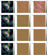 |
Fig. 4 Reconstruction results of 30Dor. (a, d, g, j) Results on a log10 scale reconstructed by SARA, AIRI, LPG, and ISCAD, respectively. (b, e, h, k) Error images on a linear scale for SARA, AIRI, LPG, and ISCAD, respectively. (c, f, i, l) Real part of the residual images on a linear scale for SARA, AIRI, LPG, and ISCAD, respectively. |
Performance of different approaches for 30Dor.
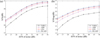 |
Fig. 5 (a) S/N and (b) S/Nlog performance of algorithms under different noise levels. |
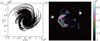 |
Fig. 6 (a) SKA baseline coverage. (b) Test image with a pixel size of 1024 × 1024 from the W28 supernova remnant, shown on a log10 scale. |
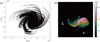 |
Fig. 7 (a) SKA baseline coverage. (b) The test image with a pixel size of 512 × 512 from the Messier 106, shown on a log10 scale. |
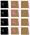 |
Fig. 8 Reconstruction results of W28. (a, d, g, j) Results on a log10 scale reconstructed by SARA, AIRI, LPG, and ISCAD, respectively. (b, e, h, k) Error images on a linear scale for SARA, AIRI, LPG, and ISCAD, respectively. (c, f, i, l) Real part of the residual images on a linear scale for SARA, AIRI, LPG, and ISCAD, respectively. |
Performance of different reconstruction methods for W28.
Performance of different reconstruction methods for Messier 106.
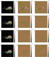 |
Fig. 9 Reconstruction results of Messier 106. (a, d, g, j) Results on a log10 scale reconstructed by SARA, AIRI, LPG, and ISCAD, respectively. (b, e, h, k) Error images on a linear scale for SARA, AIRI, LPG, and ISCAD, respectively. (c, f, i, l) Real part of the residual images in linear scale for SARA, AIRI, LPG, and ISCAD, respectively. |
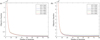 |
Fig. 10 (a, b) Convergence performance of ISCAD algorithm for W28 and Messier 106, respectively. |
5 Conclusions
The CS methods based on convex optimisation techniques such as SARA and AIRI have already demonstrated outstanding performance in radio interferometric imaging. However, convex optimisation approximately replaces the L0 norm by the L1 norm or reweighted L1 norm, which gives rise to the bias problem.
Different from convex optimisation, the proposed method adopts the continuous SCAD penalty function to approximate the L0 norm and efficiently solves the non-convex optimisation problem by using an improved proximal-gradient algorithm. The improved proximal-gradient algorithm introduces a restart strategy and an adaptive non-monotonic step-size strategy, which greatly accelerates the convergence speed of the algorithm. At the same time, the prior information of the image is used to adaptively update the regularisation parameter in the iterative process. Based on the VLA and SKA arrays, we conducted numerical simulation experiments and compared the proposed ISCAD method with state-of-the-art imaging methods such as SARA, AIRI, and LPG. The results show that ISCAD performs better than other methods in terms of reconstruction quality and computational speed.
Data availability
The code underlying this article is publicly available in https://github.com/yangxiaoch209/Radio-interferometric-Imaging.
Acknowledgements
This work is supported by the Specialized Research Fund for State Key Laboratory of Solar Activity and Space Weather. This work has used the data analysis platform of the DAocheng Radio Telescope in Chinese Meridian Project Phase II.
References
- Abdulaziz, A., Dabbech, A., & Wiaux, Y. 2019, MNRAS, 489, 1230 [Google Scholar]
- Aghabiglou, A., San Chu, C., Dabbech, A., & Wiaux, Y. 2024, ApJS, 273, 3 [NASA ADS] [CrossRef] [Google Scholar]
- Bhatnagar, S., & Cornwell, T. 2004, A&A, 426, 747 [NASA ADS] [CrossRef] [EDP Sciences] [Google Scholar]
- Birdi, J., Repetti, A., & Wiaux, Y. 2018, MNRAS, 478, 4442 [CrossRef] [Google Scholar]
- Birdi, J., Repetti, A., & Wiaux, Y. 2020, MNRAS, 492, 3509 [Google Scholar]
- Brogan, C. L., Gelfand, J., Gaensler, B., Kassim, N., & Lazio, T. 2006, ApJ, 639, L25 [Google Scholar]
- Bubeck, S., et al. 2015, Found. Trends® Mach. Learn., 8, 231 [Google Scholar]
- Candes, E. J., Eldar, Y. C., Needell, D., & Randall, P. 2011, Appl. Comput. Harmon. Anal. 31, 59 [Google Scholar]
- Candes, E. J., Wakin, M. B., & Boyd, S. P. 2008, J. Fourier Anal. Appl., 14, 877 [Google Scholar]
- Carrillo, R. E., McEwen, J. D., & Wiaux, Y. 2012, MNRAS, 426, 1223 [Google Scholar]
- Carrillo, R. E., McEwen, J. D., & Wiaux, Y. 2014, MNRAS, 439, 3591 [Google Scholar]
- Condat, L. 2014, IEEE Signal Process. Lett. 21, 985 [Google Scholar]
- Cornwell, T. J. 2008, IEEE J. Sel. Top. Signal Process., 2, 793 [Google Scholar]
- Cornwell, T. 2009, A&A, 500, 65 [NASA ADS] [CrossRef] [EDP Sciences] [Google Scholar]
- Dabbech, A., Terris, M., Jackson, A., et al. 2022, ApJ, 939, L4 [NASA ADS] [CrossRef] [Google Scholar]
- Dabbech, A., Aghabiglou, A., San Chu, C., & Wiaux, Y. 2024, ApJ, 966, L34 [NASA ADS] [CrossRef] [Google Scholar]
- Dewdney, P. E., Hall, P. J., Schilizzi, R. T., & Lazio, T. J. L. 2009, Proc. IEEE, 97, 1482 [NASA ADS] [CrossRef] [Google Scholar]
- Donoho, D. L. 2006, IEEE Trans. Inform. Theory, 52, 1289 [CrossRef] [MathSciNet] [Google Scholar]
- Fan, J., & Li, R. 2001, J. Am. Stat. Assoc., 96, 1348 [Google Scholar]
- Fessler, J., & Sutton, B. 2003, IEEE Trans. Signal Process., 51, 560 [Google Scholar]
- Garsden, H., Girard, J., Starck, J.-L., et al. 2015, A&A, 575, A90 [CrossRef] [EDP Sciences] [Google Scholar]
- Gheller, C., & Vazza, F. 2022, MNRAS, 509, 990 [Google Scholar]
- Högbom, J. 1974, A&A, 15, 417 [Google Scholar]
- Jia, X., Feng, X., Wang, W., Xu, C., & Zhang, L. 2018, Neurocomputing, 291, 71 [Google Scholar]
- Li, F., Cornwell, T. J., & de Hoog, F. 2011, A&A, 528, A31 [CrossRef] [EDP Sciences] [Google Scholar]
- Li, L., Fang, Y., Liu, L., et al. 2020, Appl. Sci., 10, 5909 [Google Scholar]
- Liu, H., Wang, T., & Liu, Z. 2022, Comput. Optim. Appl., 83, 651 [Google Scholar]
- Marjanovic, G., & Solo, V. 2012, IEEE Trans. Signal Process., 60, 5714 [Google Scholar]
- Onose, A., Carrillo, R. E., Repetti, A., et al. 2016, MNRAS, 462, 4314 [NASA ADS] [CrossRef] [Google Scholar]
- Onose, A., Dabbech, A., & Wiaux, Y. 2017, MNRAS, 469, 938 [NASA ADS] [CrossRef] [Google Scholar]
- O’donoghue, B., & Candes, E. 2015, Found. Comput. Math., 15, 715 [Google Scholar]
- Perley, R., Chandler, C., Butler, B., & Wrobel, J. 2011, ApJ, 739, L1 [NASA ADS] [CrossRef] [Google Scholar]
- Rau, U., Bhatnagar, S., Voronkov, M. A., & Cornwell, T. J. 2009, Proc. IEEE, 97, 1472 [NASA ADS] [CrossRef] [Google Scholar]
- Rich, J., De Blok, W., Cornwell, T., et al. 2008, AJ, 136, 2897 [NASA ADS] [CrossRef] [Google Scholar]
- Shen, Y., & Hu, R. 2019, Multidimens. Syst. Signal Process., 30, 257 [Google Scholar]
- Shimwell, T., Hardcastle, M., Tasse, C., et al. 2022, A&A, 659, A1 [NASA ADS] [CrossRef] [EDP Sciences] [Google Scholar]
- Terris, M., Dabbech, A., Tang, C., & Wiaux, Y. 2023, MNRAS, 518, 604 [Google Scholar]
- Thompson, A. R., Moran, J. M., & Swenson, G. W. 2017, Interferometry and Synthesis in Radio Astronomy (Springer Nature) [Google Scholar]
- Thouvenin, P.-A., Abdulaziz, A., Dabbech, A., Repetti, A., & Wiaux, Y. 2023a, MNRAS, 512, 1 [Google Scholar]
- Thouvenin, P.-A., Dabbech, A., Jiang, M., et al. 2023b, MNRAS, 521, 20 [Google Scholar]
- Wen, F., Chu, L., Liu, P., & Qiu, R. C. 2018, IEEE Access, 6, 69883 [Google Scholar]
- Wilber, A. G., Dabbech, A., Jackson, A., & Wiaux, Y. 2023a, MNRAS, 522, 5558 [Google Scholar]
- Wilber, A. G., Dabbech, A., Terris, M., Jackson, A., & Wiaux, Y. 2023b, MNRAS, 522, 5576 [Google Scholar]
- Xu, J., & Noo, F. 2022, Phys. Med. Biol. 67, 07TR07 [Google Scholar]
- Yang, X., You, X., Wu, L., et al. 2024, Sci. Sin. Phys. Mech. Astron., 54, 289514 [Google Scholar]
- Yang, X., Cheng, H., Wu, L., et al. 2025, PASP, 137, 024502 [Google Scholar]
- Zhang, L. 2018, A&A, 618, A117 [NASA ADS] [CrossRef] [EDP Sciences] [Google Scholar]
- Zhang, L., Bhatnagar, S., Rau, U., & Zhang, M. 2016, A&A, 592, A128 [NASA ADS] [CrossRef] [EDP Sciences] [Google Scholar]
- Zhang, L., Xu, L., & Zhang, M. 2020, PASP, 132, 041001 [Google Scholar]
- Zou, H., & Hastie, T. 2005, J. R. Stat. Soc. B, 67, 301 [Google Scholar]
The code can be downloaded from https://basp-group.github.io/Puri-Psi/
The code can be downloaded from https://github.com/basp-group/AIRI
The code is publicly available on the website https://github.com/yang/xiaoch209/Radio-interferometric-Imaging
Available at http://casaguides.nrao.edu/index.php
Image courtesy of NRAO/AUI and Brogan et al. (2006).
All Tables
All Figures
|
Fig. 1 Comparison of different penalty functions. |
| In the text | |
|
Fig. 2 Outputs of proximal operators corresponding to penalty functions. |
| In the text | |
|
Fig. 3 (a) VLA baseline coverage. (b) Test image from 30Dor, presented on a log10 scale. |
| In the text | |
|
Fig. 4 Reconstruction results of 30Dor. (a, d, g, j) Results on a log10 scale reconstructed by SARA, AIRI, LPG, and ISCAD, respectively. (b, e, h, k) Error images on a linear scale for SARA, AIRI, LPG, and ISCAD, respectively. (c, f, i, l) Real part of the residual images on a linear scale for SARA, AIRI, LPG, and ISCAD, respectively. |
| In the text | |
|
Fig. 5 (a) S/N and (b) S/Nlog performance of algorithms under different noise levels. |
| In the text | |
|
Fig. 6 (a) SKA baseline coverage. (b) Test image with a pixel size of 1024 × 1024 from the W28 supernova remnant, shown on a log10 scale. |
| In the text | |
|
Fig. 7 (a) SKA baseline coverage. (b) The test image with a pixel size of 512 × 512 from the Messier 106, shown on a log10 scale. |
| In the text | |
|
Fig. 8 Reconstruction results of W28. (a, d, g, j) Results on a log10 scale reconstructed by SARA, AIRI, LPG, and ISCAD, respectively. (b, e, h, k) Error images on a linear scale for SARA, AIRI, LPG, and ISCAD, respectively. (c, f, i, l) Real part of the residual images on a linear scale for SARA, AIRI, LPG, and ISCAD, respectively. |
| In the text | |
|
Fig. 9 Reconstruction results of Messier 106. (a, d, g, j) Results on a log10 scale reconstructed by SARA, AIRI, LPG, and ISCAD, respectively. (b, e, h, k) Error images on a linear scale for SARA, AIRI, LPG, and ISCAD, respectively. (c, f, i, l) Real part of the residual images in linear scale for SARA, AIRI, LPG, and ISCAD, respectively. |
| In the text | |
|
Fig. 10 (a, b) Convergence performance of ISCAD algorithm for W28 and Messier 106, respectively. |
| In the text | |
Current usage metrics show cumulative count of Article Views (full-text article views including HTML views, PDF and ePub downloads, according to the available data) and Abstracts Views on Vision4Press platform.
Data correspond to usage on the plateform after 2015. The current usage metrics is available 48-96 hours after online publication and is updated daily on week days.
Initial download of the metrics may take a while.