| Issue |
A&A
Volume 704, December 2025
|
|
|---|---|---|
| Article Number | A123 | |
| Number of page(s) | 6 | |
| Section | Astrophysical processes | |
| DOI | https://doi.org/10.1051/0004-6361/202555993 | |
| Published online | 05 December 2025 | |
Identifying long radio transients with accompanying X-Ray emission as disk-jet precessing black holes: The case of ASKAP J1832-0911
Research Center for Astronomy and Applied Mathematics, Academy of Athens, Athens 11527, Greece
⋆ Corresponding author: This email address is being protected from spambots. You need JavaScript enabled to view it.
Received:
17
June
2025
Accepted:
23
September
2025
Abstract
Aims. In this work we investigate whether the 2-min bursts every 44 min from ASKAP J1832-0911 can be explained by Lense-Thirring precession of an intermediate-mass black hole (IMBH) accretion disk launching a jet as an alternative to magnetar or white dwarf models.
Methods. We derived the Lense-Thirring period PLT = πGM/ac3r3 and solved PLT = 44 min to obtain the black hole mass, M, and dimensionless radius, r = R/Rg. We estimated the equipartition field, B, at r while assuming an advection dominated accretion flow or a magnetically arrested disk accretion model; we computed the Blandford-Znajek power, PBZ,; and we compared the resulting jet luminosity to the observed radio and X-ray fluxes at D ≈ 4.5 kpc. We also describe a coherent emission model based on a merging plasmoid close to the black hole.
Results. For a ∼ 0.3 − 0.9, an IMBH with M ∼ 103 − 105 M⊙ yields r ∼ 10 − 40 Rg and PLT = 44 min. Equipartition gives B ∼ 105 G at r, leading to PBZ ∼ 1035 − 39 erg s−1. With a radiative efficiency of ϵj ∼ 10−2 − 10−1, the predicted Ljet ∼ 1034 − 36 erg s−1 matches the observed FX ∼ 10−12 erg cm−2 s−1 and radio flux. The variability at ≲100 s could be clear evidence supporting this model.
Conclusions. The IMBH precessing-jet model simultaneously explains the periodicity, energetics, and duty cycle of ASKAP J1832-0911. Only high time resolution X-ray timing (in order to exclude ∼s pulsations) and multi-frequency radio polarimetry (to confirm a flat, low-polarization spectrum) can definitively distinguish the IMBH model from magnetar or white dwarf scenarios.
Key words: accretion / accretion disks / black hole physics / relativistic processes / stars: flare / X-rays: bursts
© The Authors 2025
 Open Access article, published by EDP Sciences, under the terms of the Creative Commons Attribution License (https://creativecommons.org/licenses/by/4.0), which permits unrestricted use, distribution, and reproduction in any medium, provided the original work is properly cited.
This article is published in open access under the Subscribe to Open model. This email address is being protected from spambots. You need JavaScript enabled to view it. to support open access publication.
1. Introduction
Long radio transients – sources whose emission appears abruptly and fades over time scales ranging from minutes to days – have long challenged our understanding of compact-object astrophysics (Hurley-Walker et al. 2022, 2023). A handful of galactic center radio transients (GCRTs), such as GCRT J1745-3009 with its 10-min bursts every 77 min, exemplify the periodic behavior on time scales of tens of minutes (Hyman et al. 2005). More recently, ASKAP J1832-0911 was discovered as a bright radio and X-ray transient located in the Scutum spiral arm at an estimated distance of 4.5 kpc. ASKAP observations have revealed 2-min long radio flares (at GHz frequencies, with peak flux densities on the order of 10 Jy) recurring every 44 min, and simultaneous X-ray observations have detected 2-min X-ray pulses (with fluxes 10−12 erg cm−2 s−1 in 0.5–10 keV) at the same 44-min cadence (Wang et al. 2025). Such a precise multiwavelength periodicity over tens of minutes is exceedingly rare among known transients.
There are two leading compact-object interpretations: a highly magnetized neutron star (magnetar) whose beamed emission sweeps past Earth for 2 min each 44-min rotation (Cooper & Wadiasingh 2024), and an ultracompact white dwarf binary in which magnetic gating produces synchronized radio and X-ray bursts every orbital period. A slowly rotating magnetar with occasional “heartbeat” flares can reproduce the observed X-ray energetics Pons & Viganò (2019), while analogous hour-period white dwarf-white dwarf binaries appear as possible progenitors of long radio flares (Qu & Zhang 2025) with X-rays (Schwope et al. 2023) or a white dwarf with a pulsar (Katz 2022). Although these models capture some aspects of the 44-min duty cycle, each faces challenges, such as maintaining a 44-min spin despite rapid magnetar spin-down or explaining coherent X-ray emission from a white dwarf shock engine over minute-long intervals.
Here, we instead propose that ASKAP J1832-0911 is powered by an intermediate-mass black hole (IMBH; M 103 − 105 M⊙) with a tilted accretion disk whose inner regions rigidly precess via the Lense-Thirring (LT) effect. In this picture, a relativistic jet sweeps across our line of sight for 2 min every 44 min, producing the observed radio and X-ray flares. IMBHs have been invoked to explain ultraluminous X-ray sources (e.g., Farrell et al. 2009), dynamical signatures in globular clusters (e.g., Gebhardt et al. 2005), and low-luminosity active galactic nuclei (AGNs) in dwarf galaxies (Mezcua 2017). Formation channels include direct collapse of Population III stars, runaway mergers in dense star clusters (Portegies Zwart & McMillan 2002), and the cores of dwarf galaxies (Reines & Volonteri 2015). If an IMBH of M 105 M⊙ resides in a Galactic plane cluster or an unrecognized dwarf satellite, its inner disk could naturally precess on a 44-min time scale at radii r 5 − 30 Rg while accumulating sufficient magnetic flux to power the observed jet luminosity. The field shows no cluster, dwarf-galaxy nucleus, or a persistent X-ray or IR source. An IMBH could instead inhabit a tidally disrupted or dissolved cluster remnant (Oh et al. 1995) or lie in a faint dwarf satellite below current detection limits.
This paper is organized as follows. In Section 2, we outline a simple geometric model for LT precession of a tilted ring or disk. We then derive the relationship between black hole mass, M; disk radius, r(=R/Rg); and precession period. Finally, we show how the 44-min cycle constrains M and r. In Section 3, we apply the model to derive viable IMBH mass ranges and disk radii, estimate the equipartition magnetic field at r and the corresponding Blandford-Znajek jet power, and compare these predictions to the observed radio and X-ray luminosities. We also discuss known AGN jet precession as a sanity check on our IMBH scaling (e.g., M87’s 11 yr cycle). In Section 4, we contrast the IMBH scenario with magnetar and white dwarf alternatives by summarizing key observational discriminants (e.g., X-ray spectral components, spin pulsations). We conclude with suggestions for targeted follow-up observations to definitively distinguish among these models.
2. Lense-Thirring precession and visibility geometry
To assess whether a tilted, rigidly precessing disk (and its jet) can naturally produce 2-min long flares every 44 min, we first derived the LT precession period for a test ring at radius R around a spinning black hole. We then constructed a simple geometric model (Maccarone 2002; Liska et al. 2018, 2019b) and related the jet’s half-opening angle and disk tilt to the observed duty cycle.
2.1. Lense-Thirring precession period
A Kerr black hole of mass M and dimensionless spin a has an angular momentum of  . A test particle (or narrow ring) at Boyer-Lindquist radius R experiences a nodal precession frequency ΩLT(R) given by (Wilkins 1972; Stella & Vietri 1998; Fragile et al. 2007)
 (1)
(1)
Hence, the LT precession period is
 (2)
(2)
Measuring distance in gravitational-radius units,  , and substituting R = r Rg into Eq. (2) gives
![Mathematical equation: $$ \begin{aligned} P_{\rm {LT}}(r) = \frac{\pi \,G\,M}{a\,c^3}\;r^3 = \bigl (1.55\times 10^{-5}\bigr )\,\frac{m}{a}\;r^3\quad [\mathrm{s} ], \end{aligned} $$](/articles/aa/full_html/2025/12/aa55993-25/aa55993-25-eq6.gif) (3)
(3)
where M = m M⊙ and G M⊙/c3 ≈ 4.9 × 10⁻⁶ s. Requiring PLT = 44 min = 2640 s yields the constraint
 (4)
(4)
2.2. Visibility geometry and duty cycle
If the inner disk at radius r is tilted by angle ψ relative to the black hole spin axis, it precesses at ΩLT. Assuming the jet is launched along the disk normal (Maccarone 2002; Fragile et al. 2007; Liska et al. 2018) and that our line of sight is inclined by i to the spin axis, the instantaneous angle, θ(t)1, between the jet axis and observer satisfies (Caproni et al. 2006; Maccarone 2002) cos θ(t) = cos ψ cos i + sin ψ sin i cos(ΩLT t). For a jet with half-opening angle α, it is visible whenever θ(t)≤α. Defining Δt as the total “on” time per cycle, PLT, one finds the following at the entry-exit points (θ = α):
 (5)
(5)
Setting Δt = 2 min and PLT = 44 min (so πΔt/PLT = π/22) shows that even modest tilts, ψ ∼ 10° −30°, and inclinations, i ∼ 30° −70°, yield small opening angle α ∼ 5° −15°, reproducing the 2 min per 44-min duty cycle (cf. Maccarone 2002; Liska et al. 2019b).
In Fig. 1 we present a schematic of the tilted accretion disk, its precessing jet cone, and the viewing geometry. An animation illustrating a disk tilt of ψ = 20.6°, a jet half-opening angle of α = 10°, and an observer inclination i = 30°, showing how the cone sweeps across our line of sight every 44 min, is available here.
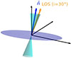 |
Fig. 1. Geometry of the precessing disk-jet system. The blue disk is tilted by ψ relative to the black hole spin axis (vertical), and the cyan cones show the jet with half-opening angle α. As the system precesses, the disk normal (blue arrow) periodically aligns with the observer’s line of sight (orange arrow), and the jet beam crosses the LOS, producing the observed 2-min flares every 44 min. An accompanying animation is available here. |
3. IMBH mass constraints, jet power, and variability
Using the LT precession relation (Eq. 4), we show that an IMBH (M ∼ 103 − 105 M⊙) naturally reproduces PLT = 44 min at radii r ∼ 5 − 30. In Appendix A we estimate the probability of these parameters being fine-tuned. We then estimate the magnetic field strength at r, compute the Blandford-Znajek jet power, compare it to the observed radio and X-ray luminosities (for D ≃ 4.5 kpc), and discuss small-scale variability and very long baseline interferometry (VLBI)-scale imaging.
3.1. Mass-radius solutions for PLT = 44 min
We needed a precession with a period of 44 min, so we plugged PLT = 2640 s into Eq. (3) and assumed a ∼ 0.3 − 0.9, which yielded  To check where the rigid precession ring is, we found
-
m = 103, a = 0.5: r = (8.53 × 10⁴)1/3 ≈ 44,
-
m = 104, a = 0.5: r = (8.53 × 10³)1/3 ≈ 20.4,
-
m = 105, a = 0.5: r = (8.53 × 10²)1/3 ≈ 9.5, and
-
m = 106, a = 0.5: r = (8.53 × 101)1/3 ≈ 4.4.
Thus, M = 103 − 105 M⊙ corresponds to r ≈ 9 − 44 Rg, which is consistent with inner-disk extents. In contrast, m ∼ 10 yields r ≈ 204. Therefore it is far outside typical XRB disks (Fragile et al. 2007; Liska et al. 2018) and cannot precess rigidly on 44-min time scales. Therefore, the IMBH regime is the only one that locates a rigidly precessing ring at r 4 − 40 Rg. However, at the small-radius end (r ≤ 4 Rg Liska et al. (2018)), frame dragging is so strong that the Bardeen-Petterson effect forces the innermost flow to realign with the black hole’s spin at the equatorial plane, potentially breaking the assumption of a perfectly rigid precession (Bardeen & Petterson 1975).
3.2. Magnetic field, power, and emission
We assumed an IMBH with M = 104 M⊙ that is in a ADAF or MAD state2 (Narayan & Yi 1994; Nemmen et al. 2007; Tchekhovskoy et al. 2011), where nearly all of the gravitational energy of the inflow is advected into the hole or carried off by magnetic stresses, rather than radiated, similar to M87, which has LM87/LEdd ≈ 10−6. The mass supply could come from Roche-lobe overflow of a donor star, which would potentially imprint on orbital modulations, or from interstellar medium capture or fallback of gas from a disrupted dense cloud.
We estimated the magnetic field of such a black hole to be around 104 G; we provide details of the estimation in Appendix F. Note that even if the accretion of an ADAF flow has a very small radiative efficiency, the respective MAD jet can have a large jet efficinecy close to 0.001–0.1, similar to M87 (Event Horizon Telescope Collaboration 2019a).
We adopted B ∼ 103 − 105 G at r ∼ 10 − 40 Rg. The Blandford-Znajek power is  (Blandford & Znajek 1977; Tchekhovskoy et al. 2010). For a = 0.5, B = 2 × 10⁴ G, and Rg = 1.5 × 109 cm, PBZ ≈ 2.1 × 1035 erg/s gives PBZ ∼ 1033 − 37 erg/s. In the Appendix D we discuss the possibility of observing the jet through VLBI. The combination of a compact emission zone (either at the jet base or within a narrow magnetospheric gap) and a low-density plasma environment minimizes Faraday rotation and depolarization, allowing intrinsically coherent radiation to retain a high degree of linear polarization3.
We describe a plausible model for coherent radio emission from IMBHs based on results of particle-in-cell (PIC) simulations from (Philippov et al. 2019). In an IMBH magnetosphere, rapid magnetic reconnection can drive coherent radio emission through plasmoid dynamics. Tearing-mode instabilities fragment a current sheet from the event horizon to the light-cylinder radius ( ) – which in a black hole magnetosphere are rather close to each other (Nathanail & Contopoulos 2014) – into a chain of magnetic islands, while strong electric fields at X-points accelerate electrons into a relativistic beam. Recent high–resolution 2D simulations have revealed tearing-mode instabilities and plasmoid formation in current sheets near the black hole horizon (Nathanail et al. 2020; Ripperda et al. 2020), while full 3D general relativistic magnetohydrodynamic studies confirm that these reconnection-driven eruptions persist in realistic accretion flows (Ripperda et al. 2022). Such rapid, localized energy releases likely seed the intermittent jet eruptions and coherent radio bursts that are observed.
When adjacent plasmoids merge, they launch fast-magnetosonic waves that act as a “wiggler” and cause the beam to bunch on wave crests and emit coherently at  where γ is the beam’s Lorentz factor. For an IMBH with M ∼ 103 − 105 M⊙, RLC/c is on scales of sub-seconds to a few seconds, so νcoh naturally falls in the 0.1–10 GHz band for a modest γ ∼ 10 − 1000 and ensures that individual burst durations remain in the millisecond to second range (see Appendix B for a note on this).
As these coherent waves escape along the low-density polar funnel, they would exhibit the narrowband spectral stripes, high polarization, and sub-structure “nanoshots” seen in pulsars and Fast radio bursts. In contrast to supermassive black holes such as M87*, whose multi-hour dynamical time scales and large RLC smear out phase coherence and push maser frequencies far below the GHz window, IMBHs hit a “sweet spot”: fast reconnection dynamics paired with emission frequencies squarely in observable radio bands. This suggests that targeted searches for fast, bright radio transients around IMBH candidates could uncover a new class of coherent maser-like signals from black hole magnetospheres.
3.3. Observed fluxes and efficiency constraints
In an MAD or ADAF state, nearly all of the gravitational energy of a near-Eddington mass supply is advected into the black hole or carried off by magnetic stresses, instead of being radiated locally. For Ṁ ≃ ṀEdd, models show radiative efficiencies as low as η ∼ 10−6 − 10−4, so the quiescent disk luminosity is  and it is undetectable at d ≃ 4.5 kpc. Meanwhile, MAD simulations have demonstrated that intermittent flux eruption events launch Poynting-flux-dominated jets with instantaneous efficiency regarding the mass accretion rate ϵj ∼ 0.01 − 1 (McKinney et al. 2012; Liska et al. 2019a). Relativistic beaming (Γ2 ∼ 4 − 25) further amplifies the apparent luminosity during each 2-min window.
In ASKAP observations, peak radio flux densities of Sν ∼ 10 Jy at ν ∼ 1.3 GHz (Wang et al. 2025) have been found. Taking a flat spectrum (α ≈ 0), the radio luminosity4 at ν = 1.3 GHz is
or νLν ∼ 3 × 1032 erg/s when integrated over a broad radio band (Δν ∼ 109 Hz). X-ray follow-ups have found FX ∼ 10−12 erg cm−2 s−1 (0.5 − 10 keV), so

Thus the combined radio and X-ray luminosity during each 2-min “on” pulse is ∼1034 − 38 erg/s. When comparing to PBZ ∼ 1035 − 39 erg/s, we observed that a modest radiative efficiency ϵj ∼ 10−2 − 10−1 suffices to power the observed fluxes.
Inside the precessing region, the jet-disk system may exhibit additional rapid variability on the local dynamical or accretion time scale. In geometric units, the light-crossing time of 1 Rg is  For M = 104 M⊙, tg ≃ 4.9 × 10⁻² s, which is very small compared with the 44-min precession. Also, short-wavelength fluctuations at the inner jet footpoint would occur on time scales of ∼10 tg (∼0.5 s) due to rapid accretion in tilted disks (Dexter & Fragile 2013). This is likely well below any detectable variability. However, flux eruption events, which are a prominent feature of strongly magnetized accretion onto a black hole, occur every 100 − 1000 tg ≈ 5 − 50 s (Liska et al. 2019b; Ripperda et al. 2022; Nathanail et al. 2025) and could be responsible for the high variability seen in the X-rays.
4. Discussion
In this work, we have invsetigated the possibility that the 2-min bursts every 44 min from ASKAP J1832-0911 can be explained by an IMBH and a precessing accretion disk launching a Blandford-Znajek jet as an alternative to magnetar or white dwarf models. The LT precession constraint,  , for a ∼ 0.3 − 0.9 yields r ∼ 10 − 40 Rg when M ∼ 103 − 105 M⊙.
The IMBH mass-radius solutions of M ∼ 103 − 105 M⊙ correspond to r ≈ 9 − 44 Rg, placing the precessing ring well within a plausible inner-disk extent. By contrast, a ∼10 − 30 M⊙ black hole would require r ∼ 443 Rg, which cannot rigidly precess on a 44 min time scale. An estimated Blandford-Znajek jet, Ljet ∼ 1033 − 38 erg/s, easily reproduces the observed ∼1034 − 36 erg/s in radio plus X-rays at D ≃ 4.5 kpc. Characteristic inner-disk time scales (tg ∼ 0.5 s, MAD flux eruptions ∼50 s) can be responsible for the rapid variability in the X-rays in the 2-min integration, and the 44-min precession remains the only coherent clock.
The main observational tests that uniquely identify a precessing-disk IMBH as the engine behind ASKAP J1832-0911 are the following (an extended discussion on this on Appendix E). All known magnetars spin in the 2–12 s range and exhibit a large-fraction soft X-ray pulsations, whereas the IMBH jet easily predicts a 2-min observed on a 44-min duty cycle. Similarly, intermediate-polar white dwarfs display spin and orbital periods of 102 − 105 s and characteristic hard bremsstrahlung spectra, neither of which are seen in this source.
Finally, the IMBH scenario naturally accommodates the finite 6-month activity seen in ASKAP J1832–0911. A sudden influx of material via a disk instability, tidal capture, or dense-cloud fallback could trigger a months-long jet-powered outburst, after which the disk drains or realigns and the flaring subsides.
Using the relation of this angle from the dot product of the line of sight and the disk normal unit vectors and allowing the disk normal to precess by an azimuthal angle ϕ = ΩLT t, we arrive at this equation.
ADAF: Advection dominated accretion flow. MAD: Magnetically arrested disk.
See Appendix C for an extra emission component coming from magnetospheric gaps from the IMBH.
A luminosity Lobs corresponds to flux 
Acknowledgments
The author was supported by the Hellenic Foundation for Research and Innovation (ELIDEK) under Grant No 23698, and by computational time granted from the National Infrastructures for Research and Technology S.A. (GRNET S.A.) in the National HPC facility – ARIS – under project ID 16033.
References
- Bardeen, J. M., & Petterson, J. A. 1975, ApJ, 195, L65 [Google Scholar]
- Belloni, T. E. 2010, Lecture Notes in Physics (Berlin Springer Verlag), 794, The Jet Paradigm [Google Scholar]
- Belloni, T. M., Klein-Wolt, M., Méndez, M., van der Klis, M., & van Paradijs, J. 2000, A&A, 355, 271 [Google Scholar]
- Blandford, R. D., & Znajek, R. L. 1977, MNRAS, 179, 433 [NASA ADS] [CrossRef] [Google Scholar]
- Caproni, A., Livio, M., Abraham, Z., & Mosquera Cuesta, H. 2006, ApJ, 653, 112 [Google Scholar]
- Clarkson, W. I., Charles, P. A., Coe, M. J., et al. 2003, MNRAS, 339, 447 [NASA ADS] [CrossRef] [Google Scholar]
- Cooper, A. J., & Wadiasingh, Z. 2024, MNRAS, 533, 2133 [Google Scholar]
- Corbel, S., Nowak, M. A., Fender, R. P., Tzioumis, A. K., & Markoff, S. 2003, A&A, 400, 1007 [NASA ADS] [CrossRef] [EDP Sciences] [Google Scholar]
- Dexter, J., & Fragile, P. C. 2013, MNRAS, 432, 2252 [NASA ADS] [CrossRef] [Google Scholar]
- Duncan, R. C., & Thompson, C. 1992, ApJ, 392, L9 [Google Scholar]
- Enoto, T., Shibata, S., Kitaguchi, T., et al. 2017, ApJS, 231, 8 [Google Scholar]
- Event Horizon Telescope Collaboration (Akiyama, K., et al.) 2019a, ApJ, 875, L4 [Google Scholar]
- Event Horizon Telescope Collaboration (Porth, O., et al.) 2019b, ApJS, 243, 26 [NASA ADS] [CrossRef] [Google Scholar]
- Farrell, S. A., Webb, N. A., Barret, D., Godet, O., & Rodrigues, J. M. 2009, Nature, 460, 73 [Google Scholar]
- Fender, R. P., Belloni, T. M., & Gallo, E. 2004, MNRAS, 355, 1105 [NASA ADS] [CrossRef] [Google Scholar]
- Fragile, P. C., & Anninos, P. 2007, ApJ, 665, 1507 [Google Scholar]
- Fragile, P. C., Blaes, O. M., Anninos, P., & Salmonson, J. D. 2007, ApJ, 668, 417 [NASA ADS] [CrossRef] [Google Scholar]
- Gebhardt, K., Rich, R. M., & Ho, L. C. 2005, ApJ, 634, 1093 [NASA ADS] [CrossRef] [Google Scholar]
- Harding, A. K., & Lai, D. 2006, Rep. Prog. Phys., 69, 2631 [NASA ADS] [CrossRef] [Google Scholar]
- Heemskerk, M. H. M., & van Paradijs, J. 1989, A&A, 223, 154 [Google Scholar]
- Hurley-Walker, N., Zhang, X., Bahramian, A., et al. 2022, Nature, 601, 526 [NASA ADS] [CrossRef] [Google Scholar]
- Hurley-Walker, N., Rea, N., McSweeney, S. J., et al. 2023, Nature, 619, 487 [NASA ADS] [CrossRef] [Google Scholar]
- Hyman, S. D., Lazio, T. J. W., Kassim, N. E., et al. 2005, Nature, 434, 50 [NASA ADS] [CrossRef] [Google Scholar]
- Kaspi, V. M. 2010, Proc. Nat. Acad. Sci., 107, 7147 [NASA ADS] [CrossRef] [Google Scholar]
- Kaspi, V. M., & Beloborodov, A. M. 2017, ARA&A, 55, 261 [Google Scholar]
- Katz, J. I. 2022, Ap&SS, 367 [Google Scholar]
- Levinson, A., & Cerutti, B. 2018, A&A, 616, A184 [NASA ADS] [CrossRef] [EDP Sciences] [Google Scholar]
- Liska, M., Hesp, C., Tchekhovskoy, A., et al. 2018, MNRAS, 474, L81 [Google Scholar]
- Liska, M. T. P., Tchekhovskoy, A., & Quataert, E. 2018, arXiv e-prints [arXiv:1809.04608] [Google Scholar]
- Liska, M., Chatterjee, K., Tchekhovskoy, A., et al. 2019a, arXiv e-prints [arXiv:1912.10192] [Google Scholar]
- Liska, M., Tchekhovskoy, A., Ingram, A., & van der Klis, M. 2019b, MNRAS, 487, 550 [CrossRef] [Google Scholar]
- Maccarone, T. 2002, MNRAS, 336, 1371 [Google Scholar]
- Makishima, K., Kubota, A., Mizuno, T., et al. 2000, ApJ, 535, 632 [NASA ADS] [CrossRef] [Google Scholar]
- Margon, B. 1984, ARA&A, 22, 507 [NASA ADS] [CrossRef] [Google Scholar]
- McKinney, J. C., Tchekhovskoy, A., & Blandford, R. D. 2012, MNRAS, 423, 3083 [Google Scholar]
- Merloni, A., Heinz, S., & di Matteo, T. 2003, MNRAS, 345, 1057 [Google Scholar]
- Mezcua, M. 2017, Int. J. Mod. Phys. D, 26, 1730021 [Google Scholar]
- Narayan, R., & Yi, I. 1994, ApJ, 428, L13 [Google Scholar]
- Nathanail, A., & Contopoulos, I. 2014, Astrophys. J., 788, 186 [Google Scholar]
- Nathanail, A., Fromm, C. M., Porth, O., et al. 2020, MNRAS, 495, 1549 [Google Scholar]
- Nathanail, A., Mizuno, Y., Contopoulos, I., et al. 2025, A&A, 693, A56 [NASA ADS] [CrossRef] [EDP Sciences] [Google Scholar]
- Nemmen, R. S., Storchi-Bergmann, T., & Eracleous, M. 2007, MNRAS, 377, 1652 [Google Scholar]
- Nixon, C., & King, A. 2016, in Lecture Notes in Physics, eds. F. Haardt, V. Gorini, U. Moschella, A. Treves, & M. Colpi (Berlin Springer Verlag), 905, 45 [Google Scholar]
- Oh, K. S., Lin, D. N. C., & Aarseth, S. J. 1995, ApJ, 442, 142 [Google Scholar]
- Patterson, J. 1994, Pub. Astron. Soc. Pac., 106, 209 [Google Scholar]
- Petterson, J. A. 1975, ApJ, 201, L61 [CrossRef] [Google Scholar]
- Philippov, A., Uzdensky, D. A., Spitkovsky, A., & Cerutti, B. 2019, ApJ, 876, L6 [NASA ADS] [CrossRef] [Google Scholar]
- Pons, J. A., & Viganò, D. 2019, Liv. Rev. Comput. Astrophys., 5, 3 [Google Scholar]
- Portegies Zwart, S. F., & McMillan, S. L. W. 2002, ApJ, 576, 899 [Google Scholar]
- Qu, Y., & Zhang, B. 2025, ApJ, 981, 34 [Google Scholar]
- Reines, A. E., & Volonteri, M. 2015, ApJ, 813, 82 [NASA ADS] [CrossRef] [Google Scholar]
- Ripperda, B., Bacchini, F., & Philippov, A. A. 2020, ApJ, 900, 100 [NASA ADS] [CrossRef] [Google Scholar]
- Ripperda, B., Liska, M., Chatterjee, K., et al. 2022, ApJ, 924, L32 [NASA ADS] [CrossRef] [Google Scholar]
- Schwope, A., Marsh, T. R., Standke, A., et al. 2023, A&A, 674, L9 [NASA ADS] [CrossRef] [EDP Sciences] [Google Scholar]
- Stella, L., & Vietri, M. 1998, ApJ, 492, L59 [NASA ADS] [CrossRef] [Google Scholar]
- Tauris, T. M., & Manchester, R. N. 1998, MNRAS, 298, 625 [NASA ADS] [CrossRef] [Google Scholar]
- Tchekhovskoy, A., Narayan, R., & McKinney, J. C. 2010, ApJ, 711, 50 [NASA ADS] [CrossRef] [Google Scholar]
- Tchekhovskoy, A., Narayan, R., & McKinney, J. C. 2011, MNRAS, 418, L79 [NASA ADS] [CrossRef] [Google Scholar]
- Turolla, R., Zane, S., & Watts, A. L. 2015, Rep. Prog. Phys., 78, 116901 [Google Scholar]
- Vos, J., Cerutti, B., Mościbrodzka, M., & Parfrey, K. 2025, Phys. Rev. Lett., 135, 015201 [Google Scholar]
- Wang, Z., Rea, N., Bao, T., et al. 2025, Nature, 619, 487 [Google Scholar]
- Warner, B. 1995, Cataclysmic Variable Stars (Cambridge University Press) [Google Scholar]
- Wilkins, D. C. 1972, Phys. Rev. D, 5, 814 [CrossRef] [Google Scholar]
- Yuan, Y., Chen, A. Y., & Luepker, M. 2025, ApJ, 985, 159 [Google Scholar]
Appendix A: Probability of observing a precessing-jet IMBH
The geometry alone makes a precessing-jet IMBH significantly rarer to detect than a typical radio pulsar. For half–opening angles of α = 10° −15°, the two antipodal jets sweep only 1.5%−3.4% of the full sky, and when coupled with the requirement that the system orientation yield the narrow 2/44 duty cycle, the overall detection probability falls to ≲1%. By contrast, normal radio pulsars typically beam into ∼10%− − 30% of the sky (e.g., Tauris & Manchester 1998), making them an order of magnitude more likely to be seen from Earth. This disparity helps explain why precessing-jet IMBHs would be intrinsically rare in radio transient surveys, even if they exist in comparable numbers to neutron-star systems.
Appendix B: More on coherent emission
We note that placing the coherent curvature peak in the GHz band requires very high Lorentz factors. Setting

with RLC ≃ 5rg/a ≈ 15 × 109 cm (for M = 104 M⊙, a = 0.5) gives
While this is an extreme Lorentz factor, PIC simulations of magnetospheric reconnection do produce plasmoids with γmax ≳ 103 − 104 in localized regions (Vos et al. 2025).
We further assume that the polar funnel is sufficiently underdense (electron densities ne ≲ 108 cm−3) and hot (Te ≳ 109 K) that both free–free and synchrotron self-absorption are negligible at 1–10 GHz. This remains our most speculative assumption, but it is consistent with numerical simulations of MAD funnel properties (Event Horizon Telescope Collaboration 2019b) in both IMBH and low luminosity AGN simulations.
Appendix C: Possibility of gap emission
In addition to the Blandford-Znajek jet, a narrow vacuum gap in the black hole magnetosphere could also provide a compact, highly ordered emission region capable of producing coherent, highly polarized bursts. In such a gap the available potential drop is  , where ΩBH = a c/2Rg is the angular frequency of the event horizon. The produced electric current through the Goldreich-Julian characteristic charge density nGJ = ΩBH B/2π e c, is IGJ ≈ nGJ e c π rg2 ∼ ΩBH B rg2/2c. So that the gap power Lgap ∼ ΔgapIGJ ∼ 1037 − 38erg/s for M ∼ 104 M⊙, B ∼ 2 × 10⁵ G, and a = 0.5. Particle-in-cell simulations of black hole gap discharges show that rapid plasma oscillations can lead to charge bunching and pair cascades (Levinson & Cerutti 2018; Yuan et al. 2025). Thus, whether emerging from the jet-launching region or from a magnetospheric gap, a compact, ordered field geometry can explain the observed coherent, highly polarized radio pulses.
Appendix D: VLBI-scale jet size and resolvability
A final test is whether the precessing jet can be spatially resolved with VLBI. If the jet originates near r ≈ 20 Rg, then its transverse radius at launch is of order

where α is the jet’s half-opening angle, say α ≃ 10° ≈0.1745 rad. Thus

Assuming the jet remains collimated on larger scales but starts with a cylindrical cross-section of radius 5 × 109 cm, its angular size at D = 4.5 kpc is

Even if the jet expands conically by a factor of 100 before becoming optically thin (i.e. radius ∼2.6 × 1011 cm), θ ∼ 7.4 μas, still below typical VLBI resolution at 1.3 GHz (∼200 μas). Only future space-VLBI at higher frequencies could hope to resolve any structure. Therefore, direct imaging of the precessing jet is effectively impossible with current VLBI; the only observable is time-dependent brightness modulation ("hot spot" lighting up as the beam swings by).
Appendix E: Discriminating between IMBH, magnetar, and white dwarf scenarios
In this section, we summarize the "smoking-gun" tests that distinguish a precessing-disk IMBH from alternative magnetar or white dwarf models, and explain why a stellar-mass (∼10 − 30 M⊙) black hole X-ray binary (XRB) is effectively ruled out-short of observing a state transition lasting months-years that temporarily erases and then restores the 2 min / 44 min pattern.
E.1. Magnetar model versus IMBH jet
All known magnetars spin with Pspin ∼ 2 − 12 s and exhibit coherent pulsations in soft X-rays (0.5-10 keV) with large pulsed fractions (∼10 − 50%) (e.g., Pons & Viganò 2019; Kaspi & Beloborodov 2017). A slowly rotating (∼44 min) magnetar would spin down catastrophically fast (Ṗ ∼ 10−9 − 10−8 s/s for B ∼ 1014 − 1015 G), making long-term stability impossible (Duncan & Thompson 1992; Harding & Lai 2006). If ASKAP J1832–0911 were a magnetar spinning at P = 2640 s, it could in principle maintain that period with only minimal spin-down over months. However, a standard dipolar field of 1014 − 1015 G would force much faster braking, so one must invoke a predominantly multipolar surface field to suppress spin-down. Even then, the key questions become how the star reached such an ultra-long period in the first place and what mechanism sustains its ongoing activity.
By contrast, an IMBH jet model predicts ∼s-scale variability; in the 2 min precession on window and, at most, high-frequency flickering on ≲102 s time scales (Liska et al. 2018). Deep, high-time-resolution X-ray timing can rule out any Pspin < 12 s.
Persistent magnetar spectra are well modeled by one or two blackbodies (kT ∼ 0.3 − 0.6 keV) plus a hard power-law tail (Γ ∼ 2 − 4) (Enoto et al. 2017; Turolla et al. 2015), with no cool (< 0.1 keV) disk component. An IMBH, however, should show a multicolor disk blackbody peaking at kTin ∼ 0.05 − 0.1 keV (for M ∼ 104 M⊙) plus a nonthermal tail from jet-disk coupling (Makishima et al. 2000; Farrell et al. 2009).
Magnetars are typically isolated or in young supernova remnants/OB associations (Kaspi 2010). A bright optical/IR counterpart showing magnetospheric pulsations (∼s) would favor a magnetar. In contrast, an IMBH in a dwarf galaxy or globular cluster may be optically faint (MV > −2) or undetected at 4.5 kpc (Mezcua 2017). Deep HST or 8 m-class imaging: detection of an OB companion or supernova remnant shell implies a magnetar; absence of a stellar counterpart, possibly a faint extended cluster, favors the IMBH.
E.2. White dwarf model versus IMBH jet
Intermediate polar white dwarfs have Pspin ∼ 102 − 103 s and orbital periods Porb ∼ 104 − 105 s. A beat between spin and orbital cannot naturally produce a strict 44 min (∼2640 s) period without fine tuning (Patterson 1994; Qu & Zhang 2025). Such systems would also exhibit coherent pulsations at the white dwarf spin (∼500 s) or orbital (∼104 s) periods in X-ray/optical light curves (Warner 1995). An IMBH jet model predicts none of these intermediate periods-only the 44 min precession and high-frequency flicker (< 102 s). Searching for 102 − 104 s pulsations can thus discriminate a white dwarf origin.
Achieving a stable Δt/P = 2/44 min duty cycle over months would require an implausible long-term phase lock between spin and orbit in a white dwarf system (Warner 1995), as tiny changes in Ṗ or mass-transfer rate would break the 44 min clock. An LT-precessing IMBH disk is expected to maintain PLT stably for 104 − 106 tg (Fragile et al. 2007; Liska et al. 2018). Monitoring the period over ≳6 months: any ΔP/P ≳ 1% drift is inconsistent with LT precession but expected for white dwarf spin evolution (Ṗ ∼ 10−11 s/s).
E.3. Low-mass XRB versus IMBH
For a stellar-mass black hole (m ∼ 10), Eq. (4) demands r ∼ 443 Rg (R ∼ 6.6 × 10³ km) to satisfy PLT = 44 min. At such radii, the viscous time scale tacc is ∼11 days (Fragile et al. 2007; Liska et al. 2019b), preventing rigid precession. Assuming a small, geometrically thick or warped mini-disks, warp communication is mediated by bending waves rather than viscous diffusion, allowing the inner annuli to precess more rapidly than a rigid-body model would predict (Fragile & Anninos 2007; Nixon & King 2016). However, even with such differential precession, maintaining a stable 2 min / 44 min duty cycle at radii of r ∼ 440 Rg poses severe coherence and damping challenges. Known XRBs precess on much longer superorbital time scales (SS 433: 162 d; Her X-1: 35 d; LMC X-4: 30 d; SMC X-1: 60 d) (Margon 1984; Petterson 1975; Heemskerk & van Paradijs 1989; Clarkson et al. 2003), which, however, are superorbital precession due to binary torques and not Lense–Thirring precession.
Moreover, a ten-solar-mass XRB jet at r ∼ 443 Rg would have too low PBZ (∼1031 − 33 erg/s) to power the observed LX ∼ 1034 − 36 erg/s (Merloni et al. 2003). In canonical XRB behavior, a transition from the hard state (jet "on") to soft state (jet quenched) occurs over hours-days (Fender et al. 2004; Corbel et al. 2003), during which the radio flares vanish and the X-ray spectrum softens. Only if ASKAP J1832-0911 were to undergo such a state transition-suppressing the 2/44 pattern for days-weeks and later restoring it-could a low-mass XRB remain viable, a behavior not yet observed in this source.
In canonical XRB behavior, a transition from the low/hard state (jet active, hard X-ray power law) to the high/soft state (jet quenched, disk-dominated spectrum) occurs over hours-days (Fender et al. 2004; Corbel et al. 2003). During this transition, the flat-spectrum radio core disappears and the nonthermal X-ray tail softens (Belloni 2010). If ASKAP J1832-0911 were a ten-solar-mass XRB, the 2 min/44 min flares would persist until such a state transition, vanish for days-weeks, and only reappear after returning to the hard state over months-years (as seen in GRS 1915+105; Belloni et al. (2000)). No prolonged "off-period" has been observed to date. In the absence of any detected state transition, a 10 − 30 M⊙ XRB interpretation is strongly disfavored. Only a future detection of jet quenching and spectral softening lasting days, followed by a re-establishment of the 2/44 pattern after years, could salvage the low-mass XRB scenario.
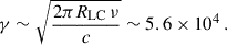
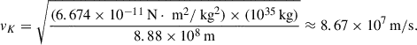
Appendix F: Estimating the magentic field of a 104 M⊙ black hole
Assuming a radiatively inefficient accretion flow (ADAF) like M87, one would expect that the black hole accretes at a very small fraction of its Eddington limit (typically ∼10−4 − 10−6 of ṀEdd). The dominant velocity of the orbiting plasma at a radius of ∼6Rg is the Keplerian velocity  ,
,
At this point, if we equate the magnetic pressure  , where
  is the permeability of free space, with the ram pressure of the disk Pram = ρvK2 we get, PB = Pram,

Solving for B, we get 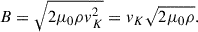
Thus,  ,
,

To arrive to the this density ρ ≈ 10−10 kg/m3), we can use the continuity equation

assuming Ṁ ≈ ∼ 10−4 − 10−6 ṀEdd at 6 Rg of a 104 M⊙, where  and ur ≈ 0.05c.
In systems like M87*, the accretion disk’s low radiative efficiency is due to energy being advected into the black hole. However, the jet’s higher efficiency comes from tapping into a separate energy reservoir: the black hole’s spin (via the Blandford-Znajek process). This means the disk and the jet can have vastly different energy conversion efficiencies.
All Figures
|
Fig. 1. Geometry of the precessing disk-jet system. The blue disk is tilted by ψ relative to the black hole spin axis (vertical), and the cyan cones show the jet with half-opening angle α. As the system precesses, the disk normal (blue arrow) periodically aligns with the observer’s line of sight (orange arrow), and the jet beam crosses the LOS, producing the observed 2-min flares every 44 min. An accompanying animation is available here. |
| In the text | |
Current usage metrics show cumulative count of Article Views (full-text article views including HTML views, PDF and ePub downloads, according to the available data) and Abstracts Views on Vision4Press platform.
Data correspond to usage on the plateform after 2015. The current usage metrics is available 48-96 hours after online publication and is updated daily on week days.
Initial download of the metrics may take a while.