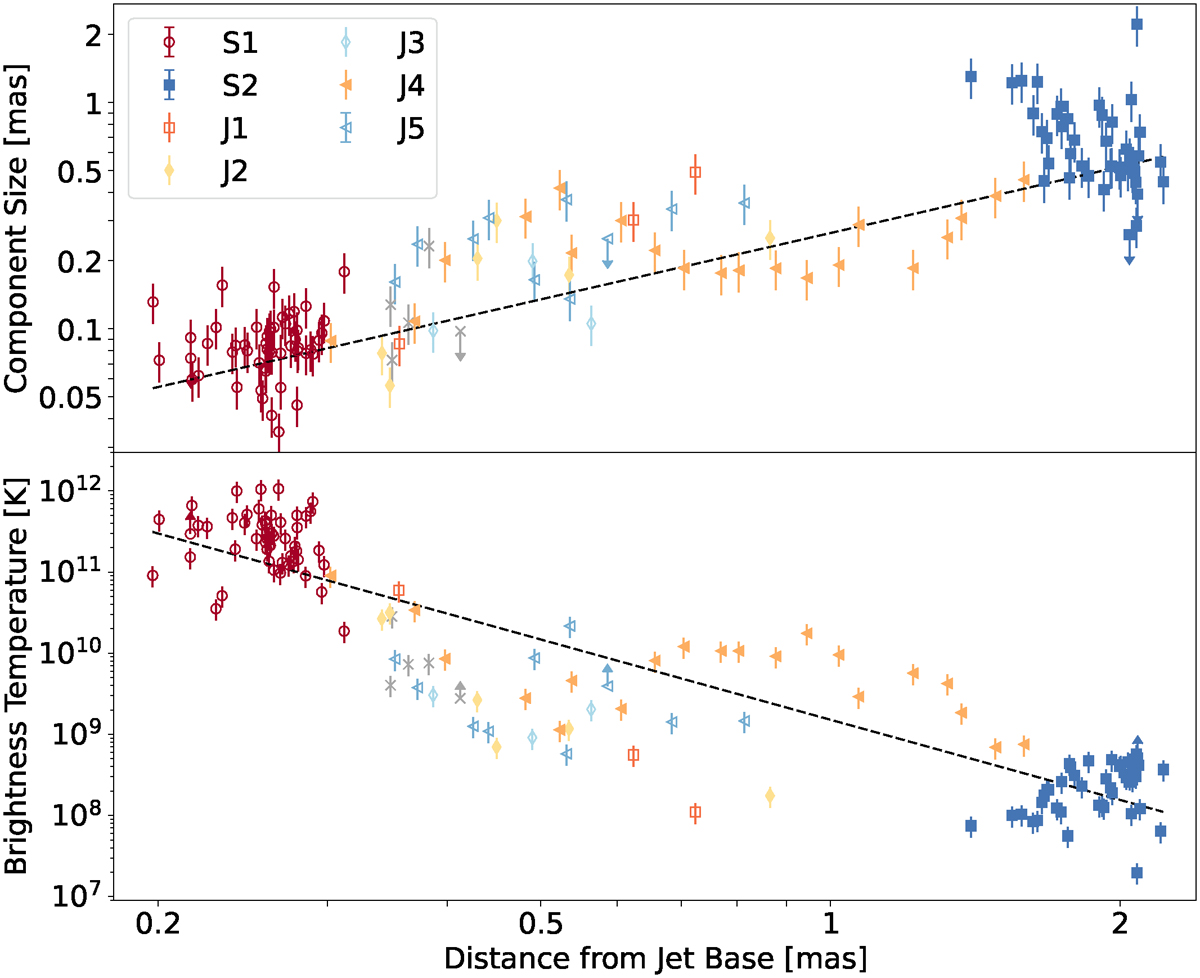
Fig. 4.
Download original image
Upper panel: jet width D, given by the FWHM size of the jet components, plotted as a function of their distance from the jet base. The dashed line is fitted via D = C(d + dc, 43, app)l, where dc, 43, app is the apparent distance of the 43 GHz core to the jet base, d is the distance from the core to the jet component, C is a constant, and l is the power law index representing the jet geometry. The best fit results in l = 0.974 ± 0.098 which is consistent with a conical jet. Lower panel: observed brightness temperature TB of the jet components plotted as a function of the components’ distances to the jet base. The dashed line is fitted via log(TB) = s ⋅ log(d + dc, 43, app)+log(C), in which dc, 43, app is the apparent distance of the 43 GHz core to the jet base and s is the brightness-temperature gradient. For dc, 43, app we used the value derived in Sect. 3.1.3. The best fit results in s = −3.31 ± 0.31 which corresponds to a conical jet in equilibrium between magnetic field strength density and electron energy density (Burd et al. 2022).
Current usage metrics show cumulative count of Article Views (full-text article views including HTML views, PDF and ePub downloads, according to the available data) and Abstracts Views on Vision4Press platform.
Data correspond to usage on the plateform after 2015. The current usage metrics is available 48-96 hours after online publication and is updated daily on week days.
Initial download of the metrics may take a while.