| Issue |
A&A
Volume 704, December 2025
|
|
|---|---|---|
| Article Number | A143 | |
| Number of page(s) | 17 | |
| Section | Extragalactic astronomy | |
| DOI | https://doi.org/10.1051/0004-6361/202556231 | |
| Published online | 05 December 2025 | |
Pinpointing the location of the γ-ray emitting region in the FSRQ 4C +01.28
1
Julius-Maximilians-Universität Würzburg, Fakultät für Physik und Astronomie, Institut für Theoretische Physik und Astrophysik, Lehrstuhl für Astronomie, Emil-Fischer-Str. 31, D-97074 Würzburg, Germany
2
Max-Planck-Institut für Radioastronomie, Auf dem Hügel 69, 53121 Bonn, Germany
3
Center for Astrophysics | Harvard & Smithsonian, Cambridge, MA 02138, USA
4
Finnish Centre for Astronomy with ESO (FINCA), University of Turku, FI-20014 Turku, Finland
5
Aalto University Metsähovi Radio Observatory, Metsähovintie 114, FI-02540 Kylmälä, Finland
6
Aalto University Department of Electronics and Nanoengineering, PL 15500, FI-00076 Aalto, Finland
7
The University of Mississippi, Department of Physics and Astronomy, Oxford, MS 38677, USA
8
Owens Valley Radio Observatory, California Institute of Technology, Pasadena, CA 91125, USA
⋆ Corresponding author: This email address is being protected from spambots. You need JavaScript enabled to view it.
Received:
3
July
2025
Accepted:
25
September
2025
Abstract
Aims. The flat-spectrum radio quasar (FSRQ) 4C +01.28 is a bright and highly variable radio and γ-ray emitter. We aim to pinpoint the location of the γ-ray emitting region within its jet in order to derive strong constraints on γ-ray emission models for blazar jets.
Methods. We use radio and γ-ray monitoring data obtained with the Atacama Large Millimeter/submillimeter Array (ALMA), the Owens Valley Radio Observatory (OVRO), the Submillimeter Array (SMA), and the Large Area Telescope on board the Fermi Gamma-ray Space Telescope (Fermi/LAT) to study the cross-correlation between γ-ray and multifrequency radio light curves. Moreover, we employ Very Long Baseline Array (VLBA) observations at 43 GHz over a period of around nine years to study the parsec-scale jet kinematics of 4C +01.28. To pinpoint the location of the γ-ray emitting region, we use a model in which outbursts shown in the γ-ray and radio light curves are produced when moving jet components pass through the γ-ray emitting and the radio core regions.
Results. We find two bright and compact newly ejected jet components that are likely associated with a high activity period visible in the Fermi/LAT γ-ray and different radio light curves. The kinematic analysis of the VLBA observations leads to a maximum apparent jet speed of βapp = 19 ± 10 and an upper limit on the viewing angle of ϕ ≲ 4°. Furthermore, we determine the power law indices that are characterizing the jet geometry, brightness temperature distribution, and core shift to be l = 0.974 ± 0.098, s = −3.31 ± 0.31, and kr = 1.09 ± 0.17, respectively, which are all in agreement with a conical jet in equipartition. A cross-correlation analysis shows that the radio light curves follow the γ-ray light curve. We pinpoint the location of the γ-ray emitting region with respect to the jet base to the range of 2.6 pc ≤ dγ ≤ 20 pc.
Conclusions. Our observational limits places the location of γ-ray production in 4C +01.28 beyond the expected extent of the broad-line region (BLR) and therefore challenges blazar-emission models that rely on inverse Compton up-scattering of BLR seed photons.
Key words: galaxies: active / galaxies: jets / gamma rays: galaxies / quasars: individual: 4C +01.28
© The Authors 2025
 Open Access article, published by EDP Sciences, under the terms of the Creative Commons Attribution License (https://creativecommons.org/licenses/by/4.0), which permits unrestricted use, distribution, and reproduction in any medium, provided the original work is properly cited.
This article is published in open access under the Subscribe to Open model. This email address is being protected from spambots. You need JavaScript enabled to view it. to support open access publication.
1. Introduction
Blazars, radio-loud active galactic nuclei (AGNs) with jets pointing towards earth, represent the largest population of extra-galactic objects in the γ-ray band (Abdo et al. 2009). They emit radiation throughout the entire electromagnetic spectrum from radio frequencies up to high γ-ray energies. However, the exact location where the γ-rays are produced within the blazar jets is still under active discussion. While the radio emission is thought to be produced by synchrotron radiation from relativistic electrons, different leptonic (e.g., Maraschi et al. 1992; Sikora et al. 1994, 2009; Ghisellini & Tavecchio 2009) and hadronic (e.g., Mannheim 1993) processes are discussed to explain the γ-ray emission. All these γ-ray emission models require seed photon fields to produce high-energy photons via inverse Compton (IC) scattering in the case of leptonic models or by photon-proton interactions in hadronic models. For IC models these seed photons can be provided by the jet’s synchrotron photons that can be up-scattered to γ-ray energies by the same electron population that is responsible for the synchrotron radiation, which is called synchrotron self-Compton (SSC) emission (e.g., Maraschi et al. 1992). Alternatively, in external Compton (EC) and hadronic emission models, external photon fields are considered. These external photon fields can be provided by UV photons from the broad-line region (BLR; e.g., Sikora et al. 1994), which is typically located ≲1 pc away from the central super massive black hole (SMBH; e.g., Zhang et al. 2007), by IR photons between the BLR and the dust torus (e.g., Sikora et al. 2009), or by photons from the cosmic microwave background (CMB; e.g., Ghisellini & Tavecchio 2009).
Due to the ubiquitous intraday variability of the γ-ray emission of blazars which indicates a compact emission region, EC scattering of BLR photons is generally favored in the class of broad-line blazars. However, the same BLR photons used for EC scattering should become targets for the γ − γ → e± process, leading to a strong cut-off in the γ-ray spectrum above ∼20 GeV, so that no emission at very high energies (VHE) ≥100 GeV should be detectable (Costamante et al. 2018). Nevertheless, such VHE emission is observed in individual quasars (e.g., Aleksić et al. 2011). Moreover, Costamante et al. (2018) find no evidence for the expected spectral curvature due to BLR absorption in a sample of broad-line blazars suggesting that the γ-ray emitting region is located outside the BLR.
Studies of statistical samples with multiwavelength and very long baseline interferometry (VLBI) information, support the idea of a γ-ray emitting region located well beyond the BLR. Jorstad et al. (2001) found a connection between γ-ray outbursts and ejections of superluminal jet components from the radio core that places the γ-ray emitting region several parsecs downstream of the central engine. This scenario is supported by several cross-correlation studies between γ-ray and radio light curves (e.g., Fuhrmann et al. 2014; Max-Moerbeck et al. 2014; Kramarenko et al. 2022) which find that the γ-ray light curves lead the radio light curves for many blazars, suggesting the γ-ray emitting region to be located upstream of the radio cores, and, in some cases, outside of the BLR’s outer edges.
In this paper, we perform a detailed individual-source study to explore the described scenario using the blazar 4C +01.28 as a laboratory. 4C +01.28 (also known as TXS 1055+018, RGB J1058+015, and 4FGL J1058.4+0133) has a redshift of z = 0.89 (Jorstad et al. 2017) and is optically classified as a FSRQ (e.g., Lister & Homan 2005; Véron-Cetty & Véron 2010). In the case of 4C +01.28, rich multifrequency radio observational data are available with the light curves showing high variability alongside outbursts occurring every 1 − 2 years (Lister et al. 1998). Interestingly, Very Long Baseline Array (VLBA) observations at 43 GHz of 4C +01.28 show the ejection of a superluminal jet component that seems to be associated with a bright γ-ray outburst (MacDonald et al. 2017). Overall, 4C +01.28 represents a perfect target to pinpoint the location of the γ-ray emitting region.
The paper is structured as follows. In Sect. 2 we present the data and the data-analysis methods. In Sect. 3 we show the results of the analysis of the 43 GHz VLBA observations (Sect. 3.1) and of the cross-correlation of multifrequency light curve data (Sect. 3.2). In Sect. 4 we discuss how the combination of the results found by the analysis of the VLBA and the multifrequency data can be used to pinpoint the location of the γ-ray emitting region in the jet of 4C +01.28. Finally, we summarize the results and draw our conclusions in Sect. 5. Throughout the paper, we use a ΛCDM cosmological model with H0 = 70 km s−1 Mpc−1, Ωm = 0.30, and ΩΛ = 0.70.
2. Observations and data analysis
2.1. VLBA data
To study the parsec-scale jet structure of 4C +01.28, we employed radio data from the Boston University (BU) Blazar Monitoring Program BEAM-ME1. This data, observed with the VLBA at 43 GHz since April 2009, has been calibrated and imaged by the BU-group using the Astronomical Image Processing System (AIPS; Greisen 1998) provided by the National Radio Astronomy Observatory (NRAO) and the CLEAN algorithm implemented in the program DIFMAP (Shepherd et al. 1997). More detailed information on the calibration and imaging process can be found in Jorstad et al. (2005), Jorstad et al. (2017), and Weaver et al. (2022).
Since in this work we focus on two newly ejected jet features that appeared in August 2015 and June 2018, and seem to be associated with a period of high γ-ray activity, we concentrate on 20 epochs observed on a similar time range, specifically between April 2015 and December 2018 (see Fig. 1). However, since Weaver et al. (2022) present an independent analysis of the 43 GHz BU data from April 2009 until December 2018 (consisting of 51 epochs), to guarantee comparability with their study, we consider the epochs starting from April 2009 as well. These additional epochs are shown in Figs. B.1–B.2.
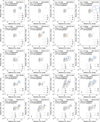 |
Fig. 1. Selected uniformly weighted 43 GHz VLBA total intensity images of the FSRQ 4C +01.28 with the fitted Gaussian components overlaid. Stot is the total integrated flux density, Speak is the highest flux density per beam, and σ is the noise level. The gray ellipse in the bottom left corner corresponds to the beam. The contours begin at 3σ and increase logarithmically by a factor of 2. The image parameters are listed in Table C.1. The images show two newly ejected jet components appearing in August 2015 (J4) and June 2018 (J5) that can be tracked back until April 2015 and February 2017, respectively. In this work we focus on these two newly ejected components. Additional plots of the epochs observed before April 2015 are shown in Appendix B in Figs. B.1–B.2. |
Although most of the images show one bright feature at the center and a jet in the northwest direction (see Fig. 1 and Figs. B.1–B.2), six epochs show unique and relatively bright features in the northern direction. Since such a structure is expected to be an artifact, in an attempt to improve them, we re-imaged them, obtaining images more in agreement with the structure seen at other epochs.
The parameters of all the analyzed epochs are reported in Table C.1. In Fig. 2, we show the resultant light curve of the total flux density, focusing on the time range October 2012 – December 2018. We assume an uncertainty of 5% of the measured flux which corresponds to the typical amplitude calibration error (Jorstad et al. 2017).
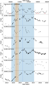 |
Fig. 2. Monthly binned γ-ray and radio light curves observed by Fermi/LAT, ALMA, SMA, and OVRO and the VLBA total flux density light curve, showing similar variability behavior. In the upper panel red arrows indicate upper limits. The vertical dashed lines represent the ejection epochs of the jet components J4 (orange) and J5 (blue) with their 1σ uncertainties shown as the orange (J4) and blue (J5) bands. The ejection of the components J4 and J5 falls into the period of high activity starting in late 2013. |
2.1.1. Image modeling
To study the time evolution of the parsec-scale jet structure of 4C +01.28, we fitted the fully calibrated visibility data of all 51 epochs with 2D Gaussian components using the MODELFIT task within DIFMAP. While the core components were fitted with elliptical Gaussians, for the jet components we used circular Gaussians. The components, overlaid on the uniformly weighted images of 4C +01.28, are plotted in Figs. B.1–B.2 as well as Fig. 1 and their parameters are listed in Table C.2. We filtered out the unresolved components, with the resolution limit calculated according to Lobanov (2005)
 (1)
(1)
where bψ is the Full Width at Half Maximum (FWHM) of the beam size along an arbitrary position angle ψ, S/N is the signal-to-noise ratio, and β = 0 for uniform weighting (for natural weighting β = 2). The S/N was calculated as Scomp/σcomp, where Scomp is the flux density of the fitted Gaussian component and σcomp is the noise level of the area that is occupied by this component. In the case of circular Gaussian jet components, bψ represents the major axes of the corresponding beams. In contrast, for the elliptical Gaussian core components, bψ was determined by measuring the FWHM along the position angle of the major and minor axes of the fitted core component. This approach establishes resolution limits for both axes individually. Whenever an axis is smaller than the corresponding resolution limit, the component is considered unresolved. By following this procedure, we find five unresolved circular jet components and two unresolved minor axes of elliptical core components.
2.1.2. Kinematic analysis
To analyze the motion of the jet components, we cross-identified the components of the different epochs and fitted their distance to the core d using the following equations:
 (2)
(2)
 (3)
(3)
in which tmid = (tmax + tmin)/2 is the midpoint of observation, dmid is the distance of the jet component to the core at tmid, μ is the angular speed, βapp is the apparent speed in units of speed of light c, and DL is the luminosity distance. For the uncertainties of the distances, we used the semi-major axes of the corresponding components, or their resolution limit for unresolved ones.
Using the same classification scheme implemented in Jorstad et al. (2017) and Weaver et al. (2022), we classified jet components with detections at ≥10 epochs and angular speed μ < 2σ as stationary features, while all other jet components were classified as moving jet features. Stationary jet components were labeled with S, moving jet components were labeled with J, and the core components were labeled with C. For moving jet components, we computed the ejection epoch t0 as the point in which the separation of the jet component to the core equals zero, namely
 (4)
(4)
2.1.3. Brightness temperature
Using the parameters of the Gaussian components given in Table C.2, we calculated the brightness temperatures TB of all components by
 (5)
(5)
in which amaj and amin are the FWHM of the major and minor axes of the Gaussian component, λ is the wavelength of observation, z is the redshift, and kB is the Boltzmann constant (Kovalev et al. 2005). Assuming relative uncertainties of 20 % for the major and minor axes and 5 % for the flux density, we calculated relative uncertainties of 29 % for the brightness temperatures. For unresolved components, the resolution limits were used, which led to a lower limit on the brightness temperatures. The brightness temperatures obtained are also listed in Table C.2 and are plotted in the upper panel of Fig. 3.
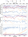 |
Fig. 3. Upper panel: observed brightness temperatures of the jet components with relative uncertainties of 29% plotted over time. The arrows denote lower limits for unresolved components. The horizontal dashed-dotted line represents the inverse Compton limit of 1012 K. The gray-shaded area denotes the range of brightness-temperature values for a jet in equipartition. The intrinsic brightness temperature of the core (blue bars) is mostly consistent with equipartition and lies only above equipartition close to the ejection epochs of moving jet components. Middle panel: flux densities of the jet components with relative uncertainties of 5% plotted over time. Lower panel: distance of the jet components relative to the core component plotted over time. The solid lines are fitted via linear regression and their gradients represent the angular speed of the corresponding component. The dashed fitted line represents an alternative kinematics model for the components J1, J2, and J3 (see Sect. 3.1.1). Components J4 and J5 seem to accelerate and are therefore fitted by two separated linear regressions each with their transition points indicated by the two vertical dotted lines. At these transition points their brightness temperatures and flux densities show a steep increase. |
2.2. Other radio data
4C +01.28 was also observed at various other radio wavelengths. Data measured by the Atacama Large Millimeter/submilimeter Array (ALMA) at band 3 (ALMA 3: 84 − 116 GHz), band 6 (ALMA 6: 211 − 275 GHz), and band 7 (ALMA 7: 275 − 373 GHz) are available at the ALMA Calibrator Source Catalogue2. Furthermore, we used data observed by the Submillimeter Array (SMA) at a wavelength of 1.3 mm that are available at the Submillimeter Calibrator List3 (Gurwell et al. 2007). Because the flux densities of the individual ALMA and SMA light curves were not measured at the same frequencies, we calculated the mean frequencies ν, with uncertainties given by the standard deviation, for all four light curves respectively. We obtain ν = (97.0 ± 6.2) GHz (ALMA 3), ν = (225.6 ± 4.8) GHz (SMA), ν = (232.5 ± 2.4) GHz (ALMA 6), and ν = (341.9 ± 8.5) GHz (ALMA 7). These mean frequencies were used for further calculations. In addition, we employed the 15 GHz light curve from the Owens Valley Radio Observatory (OVRO) blazar monitoring program (Richards et al. 2011). Note that we only used data observed from October 2012 to December 2018 in this study (see also Sect. 2.4 for more details). All these light curves are plotted in Fig. 2 and show similar structures with flux density peaks in 2014, 2015, and 2017 and a prominent flux density minimum in 2013, in agreement with the VLBA light curve.
2.3. Fermi/LAT data
In addition to radio light curves, we also used information from other wavelengths for our analysis. Specifically, 4C +01.28 was also observed by Fermi/LAT (Atwood et al. 2009) at γ-ray energies between 0.1 GeV and 100 GeV. Weekly and monthly binned γ-ray light curves are available at the Fermi/LAT Light Curve Repository4 (LCR; Abdollahi et al. 2023). We used the monthly binned light curve of 4C +01.28, which has only ∼4% of upper-limit data points (defined by test statistic (TS) values < 4; for comparison, the weekly binned light curve contains ∼26% of upper limits), which is ideal for the further analysis. Moreover, several radio light curves have relatively large gaps leading to mean sampling times more comparable to monthly binning. The γ-ray light curve measured from October 2012 to December 2018 is shown in Fig. 2. It shows high variability with prominent bright outbursts in 2014 and 2015 and a prominent flux minimum in 2013, as can also be seen in the radio light curves.
2.4. Cross-correlation analysis
Because of their similar behavior, we assume that the light curves measured by ALMA, OVRO, SMA, VLBA, and Fermi/LAT are correlated (see Fig. 2). To test this assumption, we performed a cross-correlation analysis between the Fermi/LAT γ-ray light curve and the radio ones. We neglected the ALMA 6 and VLBA light curves in this study because of their poor sampling rate compared to the other radio observations. To ensure comparability of the cross-correlation results obtained using the different radio light curves, we only used flux densities measured during the time range form October 2012 to December 2018, during which every involved light curve has measurements (Fig. 2).
Several γ-ray data points are only upper limits (indicated as red arrows in the upper panel of Fig. 2) and were neglected for the analysis (similar to the approach shown in Max-Moerbeck et al. 2014). Nonetheless, to assess the impact of their exclusion, we performed the analysis treating them as actual data points finding no significant discrepancies.
2.4.1. Cross-correlation functions
The cross-correlation function (CCF) of two evenly sampled light curves x(ti) and y(ti) as function of the time lag τ is given by
 (6)
(6)
in which  ,
,  and σx, σy are the mean values and standard deviations of x(ti) and y(ti), respectively (e.g., Fuhrmann et al. 2014).
Due to the unevenly sampled radio light curves, we used two different methods for the cross-correlation analysis, namely the Discrete Cross-Correlation Function (DCF) according to Edelson & Krolik (1988) as well as the Interpolated Cross-Correlation Function (ICF; White & Peterson 1994).
According to Edelson & Krolik (1988), at first, the set of unbinned discrete correlations (UCCFij) of all measured pairs of data points from the two investigated light curves (x(ti),y(tj)), associated with the pairwise lag Δtij = tj − ti, was computed as
 (7)
(7)
Binning these unbinned correlations in time and averaging over the pairs for which  then led to the DCF correlation coefficients at time lag τ. For this we used the average sampling time of both investigated light curves as the bin size Δτ (see, e.g., Markowitz et al. 2003). We first calculated the median sampling times of the two individual light curves separately and then used the mean value of those as Δτ.
For the ICF method introduced by White & Peterson (1994), each measured data point x(ti) was paired with the interpolated values y(ti + τ). In a second pass, the measured data points y(tj) were paired with the interpolated values x(tj − τ). For this purpose, we used a piece-wise linear interpolation with an interpolation unit of 0.5 times the average sampling time of the two light curves used to compute the ICF (e.g., Markowitz et al. 2003). Finally, averaging over both results led to the ICF correlation coefficients at time lag τ.
In order to obtain correlation coefficients that are identical to the standard linear correlation coefficient known as Pearson’s r, we calculated the DCF and ICF with local normalization. For this, we only used data points that contribute to the DCF or ICF at any particular time lag to calculate the means and standard deviations used in Eqs. (6) and (7) (see, e.g., White & Peterson 1994; Welsh 1999; Fuhrmann et al. 2014; Max-Moerbeck et al. 2014). Note that the CCF of two unrelated red-noise light curves can result in spurious correlation coefficients higher than expected (Welsh 1999; Markowitz et al. 2003), especially for time lags greater than 1/3 of the duration of the investigated light curves (Press 1978). Because of the red-noise nature of our light curves, we only calculated correlation coefficients for time lags between ±1/3 of the duration where both light curves overlap in sampling to avoid such spurious correlation coefficients.
2.4.2. Correlation significance
To determine the significance of the cross-correlation between the Fermi/LAT γ-ray and the different radio light curves, we utilized the method of mixed source correlations (e.g., Fuhrmann et al. 2014). For this purpose, we calculated the DCF and ICF between each radio light curve of 4C +01.28 and 226 unrelated γ-ray light curves of other blazars available at the Fermi/LAT LCR in the same way as described in Sect. 2.4.1. Comparing these mixed correlation coefficients with those derived using only the light curves of 4C +01.28 for each time lag, we were able to estimate the probability that the latter were produced by chance correlations.
According to Abdollahi et al. (2023), the Fermi/LAT LCR provides light curves of 1525 variable 4FGL-DR2 catalog sources with variability indices > 21.67, which corresponds to the chance of < 1% of being steady. Most of the sources are of the blazar type. However, there are also a few light curves of other source classes available at the LCR. To guarantee comparability, we only selected blazar light curves for the significance analysis. Furthermore, since we neglected upper limits in the correlation analysis (see Sect. 2.4), we set a selection cut on the average significance given by the average TS values of the γ-ray detections of the LCR blazars to ensure a high enough sampling of the γ-ray light curves. Therefore, we only chose light curves with an average significance > 47.4, which corresponds to 1/2 of the average significance of 4C +01.28 of 94.8. With these selection criteria, we find a sample of 226 blazars (without 4C +01.28) consisting of 108 FSRQs, 110 BL Lac objects, and 8 blazar candidates of uncertain type.
For all these γ-ray light curves we calculated the mixed cross-correlations neglecting upper limits. Here, we used the same bin size and interpolation unit as used for calculating the DCF and ICF using the 4C +01.28 γ-ray light curve. We then calculated the probability density function (PDF) of the distribution of the derived 226 different mixed correlation coefficients for every time lag. From these PDFs we then estimated the two sided 68.27%, 95.45%, and 99.73% confidence intervals which we refer to in the following as Gaussian equivalent 1σ, 2σ, and 3σ confidence levels, respectively.
2.4.3. Time lag uncertainties
To estimate the uncertainties of the time lags of the DCF and ICF peak coefficients, we used the Monte Carlo simulation method introduced by Peterson et al. (1998) for both methods. According to these authors, the uncertainties of the time lags depend mainly on the measurement uncertainties of the flux densities and the sampling rate of the light curves. To take the uncertainties in flux density into account, we modified each flux density measurement by random Gaussian deviates based on its individual uncertainty, which is referred to as flux randomization (FR). Moreover, to account for the sampling rate of the light curves, we used the method of random subset selection (RSS), in which we randomly discarded up to 37% of the data points of the light curve. Combining both methods, FR and RSS, into one Monte Carlo run, we simulated 1000 randomly modified pairs of light curves and calculated the DCF and ICF as explained in Sect. 2.4.1. For this purpose, we used the same bin size and interpolation unit as for the cross-correlation analysis between the original light curves. From these 1000 correlation functions we calculated the distribution of the time lags of the corresponding peak coefficients using only peak coefficients that are higher than the corresponding 1σ, 2σ, or 3σ confidence level above which the peak coefficient derived from the original light curves lay. For example, if the peak coefficient from the original light curves lay between the corresponding 2σ and 3σ confidence levels, we only used time lags at peak coefficients higher than the 2σ confidence level to calculate the distribution. We then estimated the uncertainty of the time lag at the peak coefficient from the original light curves to be the standard deviation of the derived time lag distribution.
3. Results
3.1. 43 GHz VLBA data
To analyze the motion of the jet components, we studied their position relative to the core component. Their time evolution between April 2015 and December 2018 is shown in Fig. 1, in which the fitted Gaussian components are plotted overlaid on the uniformly weighted images of 4C +01.28. We highlight how in August 2015, a new bright and compact jet feature appeared moving outwards in the jet that is identified as component J4 and can be tracked back until April 2015. In June 2018, a second moving jet component emerged. We are able to track it down to February 2017 and we identify it as component J5. In this work, we focus on these two newly ejected jet components. However, (see Sect. 3.1.1), we also study the kinematics of the epochs observed before April 2015 to ensure the comparability with an independent model-fit analysis of all 51 epochs spanning around 9 years of observations, from April 2009 until December 2018 (Weaver et al. 2022). The time evolution of the jet components of these additional epochs is shown in Figs. B.1–B.2. With the results of the kinematic analysis, we are able to calculate an upper limit for the viewing angle for 4C +01.28 (see Sect. 3.1.2). Furthermore, we also used the size and brightness temperatures of the jet components to study the jet geometry (see Sect. 3.1.3) and brightness-temperature gradient (see Sect. 3.1.4), respectively.
3.1.1. Kinematic analysis
To calculate the apparent speeds and ejection epochs of the jet components, we fitted their distances from the core with respect to the observation time as described in Sect. 2.1.2 (also see Rösch et al. 2022, for a brief discussion of this kinematics analysis). In the bottom panel of Fig. 3 the distance of the jet components to the core is plotted using the fitted Gaussians’ semi-major axes or the resolution limits for unresolved components as uncertainties. In all 51 epochs, we find a stationary component (S1) close to the core alongside a second stationary one in almost all epochs at distances of around 1.5 mas to 2 mas from the core. The position of these two components is consistent to 15 GHz MOJAVE observations (Lister et al. 2019, 2021) which also show two stationary features at similar distances.
In the epochs observed before April 2015, we also detect some additional components within the bright feature at the core region or at distances out to about 0.6 mas from the core. Because it is difficult to identify these jet components unambiguously, we consider two different models to describe their kinematics. On the one hand, we consider them as one single component moving with an apparent speed of βapp = 2.00 ± 0.61, represented by the dashed line in Fig. 3. This speed would be much lower then the speeds derived for J4 and J5 (see Table 1 and the discussion below). On the other hand, we identify them with three different jet components J1, J2, and J3 moving at apparent speeds comparable to those of J4 and J5. This second model is represented by the solid lines in Fig. 3. However, J1 and J2 can only be tracked across three epochs. Therefore, adopting the convention of Lister et al. (2009), in which at least five epochs are required to build a robust kinematics model, and considering the uncertain identification of these three components, we do not use their speeds for further analysis. Previous independent kinematic analyses (Jorstad et al. 2017; Weaver et al. 2022) identify these components as one moving jet component and a trailing feature that was formed behind it. While the speed of the moving component is comparable to the speeds of J1, J2, and J3 of our second kinematics model, the speed of the trailing feature is similar to that of the component from our first kinematics model. Therefore, this identification seems to be a combination of both models presented in this work.
Apparent speeds and ejection epochs of the jet components.
The two newly ejected jet features J4 and J5, whose kinematics are used for further analysis, seem to accelerate to higher speeds at distances downstream of ∼0.53 mas and ∼0.37 mas from the core, respectively. At smaller distances upstream of these transition points, both components seem to travel at lower constant speeds5 (see lower panel of Fig. 3). Therefore, we fitted both components with two separate linear regressions each using Eq. (2). Their transition points are indicated by the two vertical dotted lines in Fig. 3. The choice of the transition point is based on the fact that when crossing this region, the brightness temperature and flux density of J4 and J5, shown in Fig. 3, underwent a steep increase. Weaver et al. (2022) find similar results for J4 leading to comparable angular speeds, also using a broken linear fit with two transition points, located at distances consistent with our findings. Weaver et al. (2022) only identify Gaussian components with J5 at epochs between June 2018 and December 2018. In contrast to that, we also identify Gaussian components fitted to the remaining flux density shown in epochs between February 2017 and February 2018 with this component. However, the angular speeds of J5 between June 2018 and December 2018 are similar in both studies. Finally, we calculated the ejection epochs of these two components as described in Sect. 2.1.2 and for J4 we find similar results to Weaver et al. (2022).
The speeds and ejection epochs derived for robust components are listed in Table 1. Due to the large 1σ uncertainty of the ejection epoch of J5, this component could be ejected before J4, although J5 appears clearly after J4 (see Fig. 1). However, because J5 travels at a lower speed through the inner part of the jet, this scenario would be plausible. In that case, J4 would cross J5 upstream of S1. Since both components are only detected downstream of S1, this would lead to similar images.
3.1.2. Viewing angle
The apparent speed in units of speed of light βapp depends on the intrinsic jet speed in units of speed of light β and the viewing angle ϕ and is given by
 (8)
(8)
Therefore, an upper limit on ϕ can be estimated by setting β = 1 and solving Eq. (8) for ϕ, which leads to
 (9)
(9)
in which βapp, max is the largest possible apparent jet speed.
To calculate this upper limit on the viewing angle, we neglected J1, J2, and J3 because of their unclear identification and kinematic analysis. Therefore, the largest possible apparent speed within the 1σ uncertainties is βapp, max = 29 derived for J5. Using this value for βapp, max together with Eq. (9), we obtain the upper limit on the viewing angle to be ϕ ≲ 4°. This upper limit on the viewing angle is consistent to the typical viewing angle for blazar jets of ϕ < 5° derived by Jorstad et al. (2017). Furthermore, it is comparable to other estimates of the viewing angle of 4C +01.28. While Weaver et al. (2022) determine the viewing angle to be ϕ = (3.2 ± 1.0)°, using 43 GHz VLBA observations and taking the variability Doppler factor into account, Pushkarev et al. (2009) used 15 GHz VLBA observations to determine the viewing angle to be ϕ = 4.4°.
3.1.3. Jet geometry
Following the jet model introduced by Blandford & Königl (1979) and Königl (1981), we assume that the jet diameter D along the jet axis d can be described by a power law: D ∝ dl. To investigate the jet width profile, we used the FWHM of the aforementioned circular Gaussian components (see, e.g., Burd et al. 2022), with the uncertainties defined as 20% of the major axis of the respective component. The results of these measurements are presented in Fig. 4.
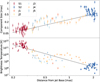 |
Fig. 4. Upper panel: jet width D, given by the FWHM size of the jet components, plotted as a function of their distance from the jet base. The dashed line is fitted via D = C(d + dc, 43, app)l, where dc, 43, app is the apparent distance of the 43 GHz core to the jet base, d is the distance from the core to the jet component, C is a constant, and l is the power law index representing the jet geometry. The best fit results in l = 0.974 ± 0.098 which is consistent with a conical jet. Lower panel: observed brightness temperature TB of the jet components plotted as a function of the components’ distances to the jet base. The dashed line is fitted via log(TB) = s ⋅ log(d + dc, 43, app)+log(C), in which dc, 43, app is the apparent distance of the 43 GHz core to the jet base and s is the brightness-temperature gradient. For dc, 43, app we used the value derived in Sect. 3.1.3. The best fit results in s = −3.31 ± 0.31 which corresponds to a conical jet in equilibrium between magnetic field strength density and electron energy density (Burd et al. 2022). |
Subsequently, we employed a single power law fit expressed as D = C(d + dc, 43, app)l, to model the data (see also Kravchenko et al. 2025; Kovalev et al. 2020). Here, d is the distance between the 43 GHz core and the jet components and dc, 43, app denotes the apparent position of the 43 GHz core from the jet base. The radio core is the most compact part of a jet and should be located at the transition region between optically thick and thin emission, where the optical depth is ≈1 (Blandford & Königl 1979; Königl 1981; Marscher et al. 2010). Note that we only used resolved components for the fit. The corresponding best-fit parameters are as follows: C = (0.265 ± 0.022) mas1 − l, dc, 43, app = (0.124 ± 0.059) mas, and l = 0.974 ± 0.098. The derived power law index l is consistent with l = 1 within its 1σ uncertainty, indicating a conical jet geometry (e.g., Kadler et al. 2004). However, it differs from l = 1.55 ± 0.07 found by Kravchenko et al. (2025) using 15 GHz MOJAVE data. They probably find a steeper gradient because they are putting more weight on larger jet scales rather than the scales probed by the 43 GHz BU data.
3.1.4. Brightness temperature
The brightness temperatures of the core and jet components are plotted in the upper panel of Fig. 3. All jet components have brightness temperatures below the inverse Compton limit of 1012 K (Kellermann & Pauliny-Toth 1969) within their uncertainties while the brightness temperatures of the core are sometimes significantly above this limit for short time intervals. Brightness temperatures above the inverse Compton limit can probably be explained by Doppler boosting. The observed brightness temperatures, TB, obs, are Doppler boosted with TB, obs = δTB, int, where TB, int is the intrinsic brightness temperature and  is the Doppler factor (e.g., Kovalev et al. 2005). Using Eq. (8) the Doppler factor can be written as
  . With this formula, we calculated the range of possible Doppler factors. We used the derived upper limit for the viewing angle of ϕ ≲ 4 and the lowest possible speed at which components travel through the core region of βapp = 1.4 measured for J5 within its 1σ uncertainty to estimate the lower limit. For the upper limit, we used βapp = 15.2 derived for J4 within its 1σ uncertainty and the lower limit of the viewing angle of ϕ = 2.2 (ϕ = 3.2 ± 1.0) presented by Weaver et al. (2022). We used the obtained range of 3.6 ≤ δ ≤ 24 to calculate the possible range of the intrinsic brightness temperatures of the core which are plotted in the upper panel of Fig. 3 (blue bars). They are clearly below the inverse Compton limit and mostly lie at values that are expected for a jet in equipartion (indicated in gray). This equipartition brightness temperature lies around 5 ⋅ 1010 K (Readhead 1994) with an upper limit of 1011 K (Singal 2009). Note that the intrinsic core brightness temperatures show values that are significantly above equipartition only at four epochs that can be associated with the ejection of J2, J3, J4, and J5, respectively.
Following the jet model introduced by Blandford & Königl (1979) and Königl (1981) and assuming that the magnetic field B, the electron density N, and the jet diameter D are given by power laws (B ∝ db, N ∝ dn, and D ∝ dl), it can be shown that the brightness temperature can also be described by a power law: TB ∝ ds. The brightness-temperature gradient s is given by (e.g., Kravchenko et al. 2025; Burd et al. 2022; Kadler et al. 2004)
 (10)
(10)
where α is the spectral index (S ∝ να) of the optically thin jet emission. To investigate this gradient for 4C +01.28, we fitted the brightness temperatures of all resolved jet components by log(TB) = s ⋅ log(d + dc, 43, app)+log(C)6 using dc, 43, app = (0.124 ± 0.059) mas derived in Sect. 3.1.3 as illustrated in the lower panel of Fig. 4. To take the uncertainty of dc, 43, app into account, we used a Monte Carlo simulation method in which we altered the value of dc, 43, app randomly within its uncertainty. With this method, we calculated 1000 different dc, 43, app values and performed 1000 different fits. We then calculated the best-fit parameters and their uncertainties to be the mean and standard deviation of the parameters derived from the different fits, which results in C = (15.4 ± 4.4)⋅108 K mas−s and s = −3.31 ± 0.31. The derived brightness-temperature gradient s is not consistent with s = −3.75 ± 0.11 found by Kravchenko et al. (2025) using 15 GHz MOJAVE data. Similar to l (see Sect. 3.1.3), this steeper gradient is likely due to the fact that Kravchenko et al. (2025) are putting more weight to larger jet scales that are not probed by the 43 GHz BU data. Assuming equipartition between the magnetic field strength density and the electron energy density, the derived brightness-temperature gradient corresponds to a conical jet (−6 ≤ s ≤ −2.5; Burd et al. 2022) and differs from a parabolic jet (−3 ≤ s ≤ −1.25; Burd et al. 2022), confirming the results presented in Sec. 3.1.3.
3.2. Cross-correlation analysis
Because of the similar behavior of the different light curves shown in Fig. 2, we computed DCF and ICF cross-correlation coefficients between the Fermi/LAT γ-ray and the ALMA, SMA, and OVRO radio light curves as described in Sect. 2.4. The results of the DCF and ICF between the Fermi/LAT and the ALMA 3 light curves are plotted in Fig. 5. Additional plots of the cross-correlation between the Fermi/LAT and the ALMA 7, SMA, and OVRO light curves are presented in Figs. A.1–A.3. One can see that the cross-correlation functions between all four pairs of light curves have their peak cross-correlation coefficients at positive time lags indicated by the solid blue lines with their uncertainties, calculated as discussed in Sect. 2.4.3, shown by the blue shaded areas. These positive time lags indicate that the radio light curves follow the γ-ray light curve. Furthermore, the DCF and ICF between each individual pair of light curves peaks at comparable time lags that are consistent with each other within their 1σ uncertainties. Note that the global peak coefficient of the DCF between the Fermi/LAT and OVRO light curves of 0.54 ± 0.14 is located at a larger time lag of (630 ± 219) days that is not consistent with the corresponding ICF time lag and with those found for the other three radio light curve. However, there is another clear peak at a time lag of (252 ± 219) days that is comparable with the other ones (see Fig. A.3). While the global peak time lag corresponds to the correlation of the radio flares in 2015 and 2017 with the γ-ray flares in 2014 and 2015, the second peak time lag corresponds to the correlation of these two radio flares to the γ-ray flares in 2015 and 2016 (see Fig. 2). Therefore, we used the second time lag for further calculations.
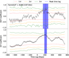 |
Fig. 5. DCF (upper panel) and ICF (lower panel) cross-correlation coefficients between the Fermi/LAT γ-ray and ALMA 3 light curves plotted over time lag. For the DCF the bin size is chosen to be 20 days, while the interpolation unit for the ICF is chosen to be 10 days (both calculated as explained in Sect. 2.4.1). Positive time lags mean that the radio light curve follows the Fermi/LAT γ-ray light curve. The time lags for the peak cross-correlation coefficients are marked by solid blue lines, with their 1σ uncertainties given by the shaded blue area. The dotted red, dashed-dotted orange, and dashed green lines correspond to the two sided Gaussian equivalent 1σ, 2σ, and 3σ confidence intervals. The DCF and ICF cross-correlation coefficients between the Fermi/LAT and ALMA 7, SMA, and OVRO light curves are plotted in Figs. A.1, A.2, and A.3, respectively. |
The peak cross-correlation coefficients derived for both methods are listed in Table 2, together with their corresponding time lags and significances. Here, one can see that the peak coefficients show a slight shift towards longer time lags with decreasing frequency of the radio light curves which could probably be explained by opacity effects (see discussion in Sect. 4.1).
Cross-correlation results derived by the DCF (top) and ICF (bottom) between the Fermi/LAT γ-ray and different radio light curves.
4. Discussion
From our study of 51-epochs of VLBA observations of 4C +01.28 at 43 GHz, we find two newly ejected jet features likely associated with the high activity period starting in late 2013 shown in the Fermi/LAT γ-ray and in several radio light curves observed at different frequencies by ALMA, OVRO, and SMA. To illustrate that, the ejection epochs derived in Sect. 3.1.1 are plotted as vertical dashed lines in Fig. 2, together with the different γ-ray and radio light curves. The orange and blue bands represent the 1σ uncertainties of the ejection epochs of J4 (orange) and J5 (blue).
In the following, we use a model in which the flares shown by the γ-ray and radio light curves occur due to opacity effects when a moving jet component passes through the γ-ray emitting region and the regions where the radio cores are located (also see Fuhrmann et al. 2014; Max-Moerbeck et al. 2014). With this model, we analyze the core shift (see Sect. 4.1) and determine the location of the γ-ray emitting region (see Sect. 4.2) in the jet of 4C +01.28.
4.1. Core shift
The absolute position of the radio core dc, ν depends on the frequency ν and is given by
 (11)
(11)
in which the power law index kr depends on the spectral index as well as on the magnetic field and particle density distributions (Königl 1981). Hence, the location of the radio core shifts upstream towards the central engine with increasing frequency (Marscher et al. 2010).
Assuming a jet in which the electron energy density N, the magnetic field strength density B, the jet diameter D, and the brightness temperature TB are given by power laws (N ∝ dn, B ∝ db, D ∝ dl, TB ∝ ds), the power law index representing the core shift is given by
 (12)
(12)
where α is the optically thin spectral index (Lobanov 1998). Further assuming a jet in equipartition between electron energy density and magnetic field strength density, which is consistent to our findings on the jet geometry (Sect. 3.1.3) and brightness temperature gradient (Sect. 3.1.4), N ∝ B2 ∝ d2b leading to n = 2b (e.g. Burd et al. 2022). Inserting n = 2b into Eqs. (10) and (12) and solving these equations for b and kr results in
 (13)
(13)
 (14)
(14)
To calculate these two power law indices, the optically thin spectral index α of the jet emission is needed. Since this α can not be determined from the data we used in this work, we used the jet spectral index presented by Hovatta et al. (2014). They calculated the spectral index at parsec scales between 8 GHz and 15 GHz VLBA observations along the ridge line of the jet of a sample of AGNs. For 4C +01.28, they found a jet spectral index that varies around −1 with its maximum and minimum at around −0.3 and −1.6 within 1σ uncertainties. Therefore, to be conservative, we used α = −1.00 ± 0.70 to calculate kr and b. Note that this α is also consistent with the jet spectral index of 4C +01.28 at smaller scales derived between quasi-simultaneous VLBI observations at 43 GHz and 86 GHz (Ricci et al., in prep.). Together with our results on the power law indices of the jet geometry, l = 0.974 ± 0.098 (see Sect. 3.1.3), and the brightness temperature gradient, s = −3.31 ± 0.31 (see Sect. 3.1.4), we obtain b = −1.07 ± 0.20 and kr = 1.09 ± 0.17. These values are both comparable with a conical jet in equipartition having a toroidal magnetic field. For such a jet b = −1, since a toroidal field scales with the jet diameter via B ∝ D−1 ∝ d−l (l = 1 for a conical jet). Note that a poloidal magnetic field scales as B ∝ D−2 ∝ d−2l, leading to b = −2 (Burd et al. 2022). Furthermore, for a freely expanding jet in equipartition between magnetic-field energy and jet particle density kr = 1 (Blandford & Königl 1979).
Using the aforementioned model, we are able to explain the behavior of the time lags derived by the cross-correlation analysis between γ-ray and radio light curves measured at different frequencies presented in Sect. 3.2 using the core shift.
The location of the radio core at frequency ν with respect to the jet base can be calculated by
 (15)
(15)
where dγ is the location of the γ-ray emitting region with respect to the jet base and dγ, ν is the distance between dγ and dc, ν. Inserting Eq. (15) into Eq. (11), we obtain  . Using dγ as reference position and using a model in which the jet component producing the γ-ray and radio outbursts travels at a constant speed through the region of the jet where the radio cores and the γ-ray emitting region are located7, we obtain
 (16)
(16)
which explains the fact that the time lags derived with the cross-correlation analysis presented in Sect. 3.2 increase with decreasing frequency across the observed radio light curves.
4.2. Location of the γ-ray emitting region
To investigate the core shift in more detail we plot the time lags listed in Table 2 as a function of the frequency in Fig. 6. Using dγ as reference position, we fitted the time lags derived by the DCF (upper panel of Fig. 6) as well as the time lags obtained by the ICF (bottom panel of Fig. 6) by
 (17)
(17)
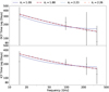 |
Fig. 6. Time lags τγ, ν derived from the DCF (upper panel) and the ICF (lower panel) plotted as a function of frequency ν. Positive time lags mean that the radio light curve follows the Fermi/LAT γ-ray light curve. To investigate the core shift, the time lags are fitted by |
where τγ is the time a newly ejected jet component needs to travel from the jet base to the γ-ray emitting region and kr = 1.09 derived from Eq. (14). The best fits of the DCF and ICF time lags are both plotted as solid dark blue lines in Fig. 6 and the parameters of both fits are listed in Table 3.
Best fit parameter and apparent locations of the γ-ray emitting region.
Assuming that a newly ejected jet component travels with constant speed from the jet base to the γ-ray emitting region and produces a γ-ray flare when crossing this region, we calculated the apparent location of the γ-ray emitting region dγ, app with respect to the jet base by
 (18)
(18)
using the results from the fits on the DCF and ICF time lags, respectively, and the speed derived by the kinematic analysis of the 43 GHz VLBA data presented in Sect. 3.1.1 and listed in Table 1.
Since the cross-correlation is driven by the flare in 2015, which can most likely be associated with the ejection of J5 (see Fig. 2), we used the angular speed of μ = (0.14 ± 0.11) mas yr−1 of J5 to calculate the apparent location of the γ-ray emitting region. Furthermore, this angular speed also corresponds to the maximum angular speed of 4C +01.28 of μ = (0.150 ± 0.014) mas yr−1 derived by using MOJAVE data observed with the VLBA at 15 GHz (Lister et al. 2019). The determined values of dγ, app are listed in Table 3 for both methods, respectively. Both values are consistent with each other within their uncertainties. Therefore, we calculated the weighted mean of the apparent location of the γ-ray emitting region to be dγ, app = 0.061 ± 0.037 mas. At a redshift of z = 0.89 (Jorstad et al. 2017), this equals to dγ, app = 0.47 ± 0.29 pc.
To determine the de-projected location of the γ-ray emitting region dγ, the viewing angle ϕ of the jet can be used, as in
 (19)
(19)
Using a similar method as for the Doppler factor (see Sect. 3.1.4), we calculated the range of dγ. For this, we used the upper limit of the viewing angle of ϕ ≲ 4° derived in Sect. 3.1.2 and the smallest possible location of the γ-ray emitting region of dγ, app, min = 0.18 pc within its 1σ uncertainty to calculate the lower limit. Furthermore, using the largest possible value for dγ, app within its 1σ uncertainty of dγ, app, max = 0.76 pc and the smallest possible viewing angle of ϕ = 2.2 (ϕ = 3.2 ± 1.0) derived by Weaver et al. (2022), we calculated the upper limit of dγ. With this method we can pinpoint the location of the γ-ray emitting region in the jet of 4C +01.28 to the range of

We highlight how such a distance is far beyond the BLR, that typically extends up to ≲1 pc (see, e.g., Zhang et al. 2007).
This result is consistent with the findings from previous studies on several other blazars by, for example, Fuhrmann et al. (2014), Max-Moerbeck et al. (2014), Kramarenko et al. (2022) using similar methods. Moreover, recent studies on different other blazars also find γ-ray emitting regions beyond the BLR using the γ-ray / optical ratio of flare energy dissipated (Kundu et al. 2025) and via modeling the spectral energy distribution (Naseef Mohammed et al. 2025; Thekkoth et al. 2024). However, there are also studies that find γ-ray absorption signatures in the light curves of several other FSRQs indicating γ-ray emitting regions inside the BLR (Agarwal et al. 2024; Das et al. 2023; Dmytriiev et al. 2025), supported also by the variability time scales observed (Das et al. 2023).
4.3. Implications for γ-ray emission models
The γ-ray emission in FSRQs is generally explained by EC scattering of seed photons originated from the BLR (Costamante et al. 2018). However, given the derived range of the de-projected location of the γ-ray emitting region of 2.6 pc ≤ dγ ≤ 20 pc and assuming a typical extend of the BLR of ≲1 pc (e.g., Zhang et al. 2007), we can rule out this emission model for the case of 4C +01.28.
This result is also supported by the derived value of the power law index representing the core shift of kr = 1.09 ± 0.17 (see Sect. 4.1). For a freely expanding jet in equipartition between magnetic-field energy and jet particle density kr = 1 (Blandford & Königl 1979). However, kr can reach 2.5 in regions with steep pressure gradients and can become even larger in the presence of external density gradients which are present in the BLR (Lobanov 1998). Therefore, we investigated how kr would change if the γ-ray emitting region was located closer to the jet base inside the BLR. The BLR typically extends from a few to a few tens of light-days, translating into 0.01 pc to 0.1 pc, for low-luminosity AGNs and from several tens to hundreds of light-days (0.1 pc to 1 pc) for high-luminosity quasars (e.g., Raimundo et al. 2020; Kaspi et al. 2000; Zhang et al. 2007). Hence, we calculated the hypothetical values that kr would have if the γ-ray emitting region was located at distances of 1 pc, 0.1 pc, and 0.01 pc from the jet base, respectively. For this purpose, we increased kr = 1.09 incrementally by steps of 0.001, fitted the DCF and ICF time lags, respectively, by Eq. (17) using the increased kr-values, and calculated the lower limit of the de-projected location of the γ-ray emitting region dγ as explained in Sect. 4.2 until dγ, min reached the above mentioned distances. With this method we find that the γ-ray emitting region would shift upstream in the jet to dγ, min ≤ 1 pc for kr ≥ 1.88 (dashed-dotted red lines in Fig. 6), dγ, min ≤ 0.1 pc for kr ≥ 2.23 (dotted light blue lines in Fig. 6), and dγ, min ≤ 0.01 pc for kr ≥ 2.26 (dashed orange lines in Fig. 6), meaning that kr would have been greater than the derived value of kr = 1.09 ± 0.17, if the γ-ray emitting region was located inside the BLR, reaching values of kr ≳ 2, in accordance with Lobanov (1998).
However, alternatively to EC scattering on BLR photons, the γ-ray emission could be produced via SSC scattering (e.g., Maraschi et al. 1992), EC scattering on IR photons originated between the BLR and the dusty torus (e.g., Sikora et al. 2009), EC scattering on CMB photons (e.g., Ghisellini & Tavecchio 2009), or via hadronic emission models (e.g., Mannheim 1993). Furthermore, given the spine-sheath structure of the jet of 4C +01.28 detected by Attridge et al. (1999) and Pushkarev et al. (2005), the seed photon field could also be provided by the jet sheath. MacDonald et al. (2015) develop a model in which synchrotron electrons from an emitting region in the jet sheath are inverse-Compton scattered by electrons of a jet component that propagates relativistically along the jet spine. Within the scope of this model, MacDonald et al. (2017) are able to explain an orphan γ-ray flare by 4C +01.28 in February 2014, as well as different other orphan γ-ray flares by several other luminous blazars.
5. Summary
In this study, we combined a kinematic analysis of 43 GHz VLBA observations of 4C +01.28 with a cross-correlation analysis between the Fermi/LAT γ-ray and several radio light curves observed with ALMA, SMA, and OVRO at different frequencies, to calculate the location of the γ-ray emitting region in the jet of 4C +01.28. Our findings are as follows:
-
Investigating 51 epochs of 4C +01.28 observed with the VLBA at 43 GHz over a period of around nine years from April 2009 until December 2018, we find two new prominent jet features, J4 and J5, that were ejected in 2014.51 ± 0.30 and 2015.4 ± 1.7, respectively. These newly ejected components can be associated with two bright flares shown in the Fermi/LAT γ-ray and several radio light curves observed by ALMA, SMA, and OVRO at different frequencies.
-
Using the maximum speed of βapp = 19 ± 10 derived for J5, we calculated the upper limit of the viewing angle of the jet of 4C +01.28 to be ϕ ≲ 4°, in agreement with findings from Pushkarev et al. (2005), Jorstad et al. (2017), and Weaver et al. (2022).
-
To analyze the jet geometry and brightness-temperature gradient, we fitted the FWHM of the Gaussian components, parameterizing the jet width, and the brightness temperatures with respect to their distance to the jet base in terms of power laws, leading to power law indices of l = 0.974 ± 0.098 and s = −3.31 ± 0.31, respectively. Both values are consistent with a conical jet (l = 1) in equipartition between the magnetic field strength density and the electron energy density (−6 ≤ s ≤ −2.5; Burd et al. 2022).
-
The cross-correlation analysis between the Fermi/LAT γ-ray light curve and several radio light curves observed at different frequencies, results in positive time lags, which means that the γ-ray light curve leads the radio light curves.
-
Using the derived power law indices representing the jet geometry and the brightness-temperature gradient, we calculated the power law index for the core shift as kr = 1.09 ± 0.17. This power law index is also consistent with a conical jet in equipartition (kr = 1; Lobanov 1998).
-
Combining the results of the kinematic analysis of the 43 GHz VLBA observations with those of the cross-correlation analysis we are able to pinpoint the location of the γ-ray emitting region within the jet of 4C +01.28. For this, we used a model similar to Fuhrmann et al. (2014) and Max-Moerbeck et al. (2014) in which the outbursts shown by the different light curves were produced when J4 and J5 passed through the γ-ray emitting region and the frequency-dependent radio cores. We obtain the possible range of de-projected locations of the γ-ray emitting region with respect to the jet base of 2.6 pc ≤ dγ ≤ 20 pc, which is far beyond the BLR which typically extends up to ≲1 pc (see, e.g., Zhang et al. 2007). This result is in contradiction with blazar-emission models that rely on inverse Compton up-scattering of seed photons from the BLR.
Data availability
Table C.2 and the FITS files of the images shown in Figs. 1, B.1, and B.2 are available at https://cdsarc.cds.unistra.fr/viz-bin/cat/J/A+A/704/A143
For the discussion (Sect. 4), we assume that these constant speeds even persisted further upstream.
Since the brightness temperatures of the jet components range over ∼7 orders of magnitude and we assume relative uncertainties of 29%, higher brightness temperatures have larger uncertainties. A simple weighted ( ) power-law fit of the form TB = C(d + dc, 43, app)s would therefore provide an s-value that is too small, because smaller brightness temperatures would have larger weights which would pull the fit towards smaller brightness temperatures.
In Sect. 3.1.1 we find that the two newly ejected components J4 and J5 moved at constant speeds in the inner jet and accelerated to higher speeds downstream at distances ≳0.37 mas from the 43 GHz core. Here, we assume that these constant speeds even persisted further upstream, from the jet base up to the 43 GHz core.
Acknowledgments
We thank the anonymous referee for their helpful comments and suggestions which improved the manuscript. We thank S. G. Jorstad, A. P. Marscher and Z. R. Weaver for helpful discussions and comments on the kinematic analysis. F. R., M. K. and L. R. acknowledge support from the Deutsche Forschungsgemeinschaft (DFG, grants 434448349 and 443220636 [FOR5195: Relativistic Jets in Active Galaxies]). T. H. was supported by Academy of Finland projects 317383, 320085, 345899, and 362571. This study makes use of the following ALMA data: ADS/JAO.ALMA#2011.0.00001.CAL. ALMA is a partnership of ESO (representing its member states), NSF (USA) and NINS (Japan), together with NRC (Canada), MOST and ASIAA (Taiwan), and KASI (Republic of Korea), in cooperation with the Republic of Chile. The Joint ALMA Observatory is operated by ESO, AUI/NRAO and NAOJ. This study makes use of VLBA data from the VLBA-BU Blazar Monitoring Program (BEAM-ME and VLBA-BU-BLAZAR; http://www.bu.edu/blazars/BEAM-ME.html), funded by NASA through the Fermi Guest Investigator Program. The VLBA is an instrument of the National Radio Astronomy Observatory, which is a facility of the National Science Foundation operated by Associated Universities, Inc. The Submillimeter Array is a joint project between the Smithsonian Astrophysical Observatory and the Academia Sinica Institute of Astronomy and Astrophysics and is funded by the Smithsonian Institution and the Academia Sinica. We recognize that Maunakea is a culturally important site for the indigenous Hawaiian people; we are privileged to study the cosmos from its summit.
References
- Abdo, A. A., Ackermann, M., Ajello, M., et al. 2009, ApJ, 700, 597 [CrossRef] [Google Scholar]
- Abdollahi, S., Ajello, M., Baldini, L., et al. 2023, ApJS, 265, 31 [NASA ADS] [CrossRef] [Google Scholar]
- Agarwal, S., Shukla, A., Mannheim, K., Vaidya, B., & Banerjee, B. 2024, ApJ, 968, L1 [NASA ADS] [CrossRef] [Google Scholar]
- Aleksić, J., Antonelli, L. A., Antoranz, P., et al. 2011, ApJ, 730, L8 [Google Scholar]
- Attridge, J. M., Roberts, D. H., & Wardle, J. F. C. 1999, ApJ, 518, L87 [NASA ADS] [CrossRef] [Google Scholar]
- Atwood, W. B., Abdo, A. A., Ackermann, M., et al. 2009, ApJ, 697, 1071 [CrossRef] [Google Scholar]
- Blandford, R. D., & Königl, A. 1979, ApJ, 232, 34 [Google Scholar]
- Burd, P. R., Kadler, M., Mannheim, K., et al. 2022, A&A, 660, A1 [NASA ADS] [CrossRef] [EDP Sciences] [Google Scholar]
- Costamante, L., Cutini, S., Tosti, G., Antolini, E., & Tramacere, A. 2018, MNRAS, 477, 4749 [Google Scholar]
- Das, A. K., Mondal, S. K., & Prince, R. 2023, MNRAS, 521, 3451 [Google Scholar]
- Dmytriiev, A., Acharyya, A., & Böttcher, M. 2025, ApJ, 983, 175 [Google Scholar]
- Edelson, R. A., & Krolik, J. H. 1988, ApJ, 333, 646 [Google Scholar]
- Fuhrmann, L., Larsson, S., Chiang, J., et al. 2014, MNRAS, 441, 1899 [NASA ADS] [CrossRef] [Google Scholar]
- Ghisellini, G., & Tavecchio, F. 2009, MNRAS, 397, 985 [Google Scholar]
- Greisen, E. W. 1998, in Astronomical Data Analysis Software and Systems VII, eds. R. Albrecht, R. N. Hook, & H. A. Bushouse, ASP Conf. Ser., 145, 204 [NASA ADS] [Google Scholar]
- Gurwell, M. A., Peck, A. B., Hostler, S. R., Darrah, M. R., & Katz, C. A. 2007, in From Z-Machines to ALMA: (Sub)Millimeter Spectroscopy of Galaxies, eds. A. J. Baker, J. Glenn, A. I. Harris, J. G. Mangum, & M. S. Yun, ASP Conf. Ser., 375, 234 [NASA ADS] [Google Scholar]
- Hovatta, T., Aller, M. F., Aller, H. D., et al. 2014, AJ, 147, 143 [Google Scholar]
- Jorstad, S. G., Marscher, A. P., Mattox, J. R., et al. 2001, ApJ, 556, 738 [NASA ADS] [CrossRef] [Google Scholar]
- Jorstad, S. G., Marscher, A. P., Lister, M. L., et al. 2005, AJ, 130, 1418 [Google Scholar]
- Jorstad, S. G., Marscher, A. P., Morozova, D. A., et al. 2017, ApJ, 846, 98 [Google Scholar]
- Kadler, M., Ros, E., Lobanov, A. P., Falcke, H., & Zensus, J. A. 2004, A&A, 426, 481 [NASA ADS] [CrossRef] [EDP Sciences] [Google Scholar]
- Kaspi, S., Smith, P. S., Netzer, H., et al. 2000, ApJ, 533, 631 [Google Scholar]
- Kellermann, K. I., & Pauliny-Toth, I. I. K. 1969, ApJ, 155, L71 [NASA ADS] [CrossRef] [Google Scholar]
- Königl, A. 1981, ApJ, 243, 700 [Google Scholar]
- Kovalev, Y. Y., Kellermann, K. I., Lister, M. L., et al. 2005, AJ, 130, 2473 [Google Scholar]
- Kovalev, Y. Y., Pushkarev, A. B., Nokhrina, E. E., et al. 2020, MNRAS, 495, 3576 [NASA ADS] [CrossRef] [Google Scholar]
- Kramarenko, I. G., Pushkarev, A. B., Kovalev, Y. Y., et al. 2022, MNRAS, 510, 469 [Google Scholar]
- Kravchenko, E. V., Pashchenko, I. N., Homan, D. C., et al. 2025, MNRAS, 538, 2008 [Google Scholar]
- Kundu, M., Bala, A., Barat, S., & Chatterjee, R. 2025, MNRAS [Google Scholar]
- Lister, M. L., & Homan, D. C. 2005, AJ, 130, 1389 [NASA ADS] [CrossRef] [Google Scholar]
- Lister, M. L., Marscher, A. P., & Gear, W. K. 1998, ApJ, 504, 702 [Google Scholar]
- Lister, M. L., Cohen, M. H., Homan, D. C., et al. 2009, AJ, 138, 1874 [NASA ADS] [CrossRef] [Google Scholar]
- Lister, M. L., Homan, D. C., Hovatta, T., et al. 2019, ApJ, 874, 43 [NASA ADS] [CrossRef] [Google Scholar]
- Lister, M. L., Homan, D. C., Kellermann, K. I., et al. 2021, ApJ, 923, 30 [NASA ADS] [CrossRef] [Google Scholar]
- Lobanov, A. P. 1998, A&A, 330, 79 [NASA ADS] [Google Scholar]
- Lobanov, A. P. 2005, A&A, submitted [arXiv:astro-ph/0503225] [Google Scholar]
- MacDonald, N. R., Marscher, A. P., Jorstad, S. G., & Joshi, M. 2015, ApJ, 804, 111 [Google Scholar]
- MacDonald, N. R., Jorstad, S. G., & Marscher, A. P. 2017, ApJ, 850, 87 [Google Scholar]
- Mannheim, K. 1993, A&A, 269, 67 [NASA ADS] [Google Scholar]
- Maraschi, L., Ghisellini, G., & Celotti, A. 1992, ApJ, 397, L5 [CrossRef] [Google Scholar]
- Markowitz, A., Edelson, R., & Vaughan, S. 2003, ApJ, 598, 935 [NASA ADS] [CrossRef] [Google Scholar]
- Marscher, A. P. 2010, in Jets in Active Galactic Nuclei, in The Jet Paradigm - From Microquasars to Quasars, T. Belloni, Lecture Notes in Physics, 794, 173 [Google Scholar]
- Max-Moerbeck, W., Hovatta, T., Richards, J. L., et al. 2014, MNRAS, 445, 428 [Google Scholar]
- Naseef Mohammed, P. N., Aminabi, T., Baheeja, C., et al. 2025, J. High Energy Astrophys., 47, 100365 [Google Scholar]
- Peterson, B. M., Wanders, I., Horne, K., et al. 1998, PASP, 110, 660 [Google Scholar]
- Press, W. H. 1978, Comments Astrophys., 7, 103 [NASA ADS] [Google Scholar]
- Pushkarev, A. B., Gabuzda, D. C., Vetukhnovskaya, Y. N., & Yakimov, V. E. 2005, MNRAS, 356, 859 [Google Scholar]
- Pushkarev, A. B., Kovalev, Y. Y., Lister, M. L., & Savolainen, T. 2009, A&A, 507, L33 [NASA ADS] [CrossRef] [EDP Sciences] [Google Scholar]
- Raimundo, S. I., Vestergaard, M., Goad, M. R., et al. 2020, MNRAS, 493, 1227 [Google Scholar]
- Readhead, A. C. S. 1994, ApJ, 426, 51 [Google Scholar]
- Richards, J. L., Max-Moerbeck, W., Pavlidou, V., et al. 2011, ApJS, 194, 29 [Google Scholar]
- Rösch, F., Kadler, M., Ros, E., et al. 2022, European VLBI Network Mini-Symposium and Users’ Meeting 2021, 1 [Google Scholar]
- Shepherd, M. C. 1997, in Astronomical Data Analysis Software and Systems VI, eds. G. Hunt, & H. Payne, ASP Conf. Ser., 125, 77. [Google Scholar]
- Sikora, M., Begelman, M. C., & Rees, M. J. 1994, ApJ, 421, 153 [Google Scholar]
- Sikora, M., Stawarz, Ł., Moderski, R., Nalewajko, K., & Madejski, G. M. 2009, ApJ, 704, 38 [CrossRef] [Google Scholar]
- Singal, A. K. 2009, ApJ, 703, L109 [NASA ADS] [CrossRef] [Google Scholar]
- Thekkoth, A., Baheeja, C., Sahayanathan, S. C. D. R., 2024, J. High Energy Astrophys., 42, 115 [Google Scholar]
- Véron-Cetty, M. P., & Véron, P. 2010, A&A, 518, A10 [Google Scholar]
- Weaver, Z. R., Jorstad, S. G., Marscher, A. P., et al. 2022, ApJS, 260, 12 [NASA ADS] [CrossRef] [Google Scholar]
- Welsh, W. F. 1999, PASP, 111, 1347 [Google Scholar]
- White, R. J., & Peterson, B. M. 1994, PASP, 106, 879 [NASA ADS] [CrossRef] [Google Scholar]
- Zhang, X.-G., Dultzin-Hacyan, D., & Wang, T.-G. 2007, MNRAS, 374, 691 [Google Scholar]
Appendix A: Additional plots of the cross-correlation analysis
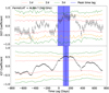 |
Fig. A.1. DCF (upper panel) and ICF (lower panel) cross-correlation coefficients between the Fermi/LAT γ-ray and ALMA 7 light curves plotted over time lag. For the DCF the bin size is chosen to be 21 days, while the interpolation unit for the ICF is chosen to be 10 days (both calculated as explained in Sect. 2.4.1). Positive time lags mean that the radio light curve follows the Fermi/LAT γ-ray light curve. The time lags for the peak cross-correlation coefficients are marked by solid blue lines, with their 1σ uncertainties given by the shaded blue area. The dotted red, dashed-dotted orange, and dashed green lines correspond to the two sided Gaussian equivalent 1σ, 2σ, and 3σ confidence intervals. |
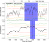 |
Fig. A.2. DCF (upper panel) and ICF (lower panel) cross-correlation coefficients between the Fermi/LAT γ-ray and SMA light curves plotted over time lag. For the DCF the bin size is chosen to be 18 days, while the interpolation unit for the ICF is chosen to be 9 days (both calculated as explained in Sect. 2.4.1). Positive time lags mean that the radio light curve follows the Fermi/LAT γ-ray light curve. The time lags for the peak cross-correlation coefficients are marked by solid blue lines, with their 1σ uncertainties given by the shaded blue area. The dotted red, dashed-dotted orange, and dashed green lines correspond to the two sided Gaussian equivalent 1σ, 2σ, and 3σ confidence intervals. |
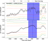 |
Fig. A.3. DCF (upper panel) and ICF (lower panel) cross-correlation coefficients between the Fermi/LAT γ-ray and OVRO light curves plotted over time lag. For the DCF the bin size is chosen to be 18 days, while the interpolation unit for the ICF is chosen to be 9 days (both calculated as explained in Sect. 2.4.1). Positive time lags mean that the radio light curve follows the Fermi/LAT γ-ray light curve. The time lags for the peak cross-correlation coefficients are marked by solid blue lines, with their 1σ uncertainties given by the shaded blue area. The dotted red, dashed-dotted orange, and dashed green lines correspond to the two sided Gaussian equivalent 1σ, 2σ, and 3σ confidence intervals. Note that we did not choose the DCF time lag of the global peak, since this time lag would not be consistent with the one of the ICF as well as those derived for the other light curves (see Sect. 3.2 for details). |
Appendix B: Additional 43 GHz VLBA images
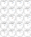 |
Fig. B.1. Uniformly weighted 43 GHz VLBA total intensity images of the FSRQ 4C +01.28 with the fitted Gaussian components overlaid. Stot is the total integrated flux density, Speak is the highest flux density per beam, and σ is the noise level. The gray ellipse in the bottom left corner corresponds to the beam. The contours begin at 3σ and increase logarithmically by a factor of 2. The image parameters are listed in Table C.1. |
Appendix C: Additional tables
Image parameters of the uniformly weighted 43 GHz VLBA observations.
All Tables
Cross-correlation results derived by the DCF (top) and ICF (bottom) between the Fermi/LAT γ-ray and different radio light curves.
All Figures
|
Fig. 1. Selected uniformly weighted 43 GHz VLBA total intensity images of the FSRQ 4C +01.28 with the fitted Gaussian components overlaid. Stot is the total integrated flux density, Speak is the highest flux density per beam, and σ is the noise level. The gray ellipse in the bottom left corner corresponds to the beam. The contours begin at 3σ and increase logarithmically by a factor of 2. The image parameters are listed in Table C.1. The images show two newly ejected jet components appearing in August 2015 (J4) and June 2018 (J5) that can be tracked back until April 2015 and February 2017, respectively. In this work we focus on these two newly ejected components. Additional plots of the epochs observed before April 2015 are shown in Appendix B in Figs. B.1–B.2. |
| In the text | |
|
Fig. 2. Monthly binned γ-ray and radio light curves observed by Fermi/LAT, ALMA, SMA, and OVRO and the VLBA total flux density light curve, showing similar variability behavior. In the upper panel red arrows indicate upper limits. The vertical dashed lines represent the ejection epochs of the jet components J4 (orange) and J5 (blue) with their 1σ uncertainties shown as the orange (J4) and blue (J5) bands. The ejection of the components J4 and J5 falls into the period of high activity starting in late 2013. |
| In the text | |
|
Fig. 3. Upper panel: observed brightness temperatures of the jet components with relative uncertainties of 29% plotted over time. The arrows denote lower limits for unresolved components. The horizontal dashed-dotted line represents the inverse Compton limit of 1012 K. The gray-shaded area denotes the range of brightness-temperature values for a jet in equipartition. The intrinsic brightness temperature of the core (blue bars) is mostly consistent with equipartition and lies only above equipartition close to the ejection epochs of moving jet components. Middle panel: flux densities of the jet components with relative uncertainties of 5% plotted over time. Lower panel: distance of the jet components relative to the core component plotted over time. The solid lines are fitted via linear regression and their gradients represent the angular speed of the corresponding component. The dashed fitted line represents an alternative kinematics model for the components J1, J2, and J3 (see Sect. 3.1.1). Components J4 and J5 seem to accelerate and are therefore fitted by two separated linear regressions each with their transition points indicated by the two vertical dotted lines. At these transition points their brightness temperatures and flux densities show a steep increase. |
| In the text | |
|
Fig. 4. Upper panel: jet width D, given by the FWHM size of the jet components, plotted as a function of their distance from the jet base. The dashed line is fitted via D = C(d + dc, 43, app)l, where dc, 43, app is the apparent distance of the 43 GHz core to the jet base, d is the distance from the core to the jet component, C is a constant, and l is the power law index representing the jet geometry. The best fit results in l = 0.974 ± 0.098 which is consistent with a conical jet. Lower panel: observed brightness temperature TB of the jet components plotted as a function of the components’ distances to the jet base. The dashed line is fitted via log(TB) = s ⋅ log(d + dc, 43, app)+log(C), in which dc, 43, app is the apparent distance of the 43 GHz core to the jet base and s is the brightness-temperature gradient. For dc, 43, app we used the value derived in Sect. 3.1.3. The best fit results in s = −3.31 ± 0.31 which corresponds to a conical jet in equilibrium between magnetic field strength density and electron energy density (Burd et al. 2022). |
| In the text | |
|
Fig. 5. DCF (upper panel) and ICF (lower panel) cross-correlation coefficients between the Fermi/LAT γ-ray and ALMA 3 light curves plotted over time lag. For the DCF the bin size is chosen to be 20 days, while the interpolation unit for the ICF is chosen to be 10 days (both calculated as explained in Sect. 2.4.1). Positive time lags mean that the radio light curve follows the Fermi/LAT γ-ray light curve. The time lags for the peak cross-correlation coefficients are marked by solid blue lines, with their 1σ uncertainties given by the shaded blue area. The dotted red, dashed-dotted orange, and dashed green lines correspond to the two sided Gaussian equivalent 1σ, 2σ, and 3σ confidence intervals. The DCF and ICF cross-correlation coefficients between the Fermi/LAT and ALMA 7, SMA, and OVRO light curves are plotted in Figs. A.1, A.2, and A.3, respectively. |
| In the text | |
|
Fig. 6. Time lags τγ, ν derived from the DCF (upper panel) and the ICF (lower panel) plotted as a function of frequency ν. Positive time lags mean that the radio light curve follows the Fermi/LAT γ-ray light curve. To investigate the core shift, the time lags are fitted by |
| In the text | |
|
Fig. A.1. DCF (upper panel) and ICF (lower panel) cross-correlation coefficients between the Fermi/LAT γ-ray and ALMA 7 light curves plotted over time lag. For the DCF the bin size is chosen to be 21 days, while the interpolation unit for the ICF is chosen to be 10 days (both calculated as explained in Sect. 2.4.1). Positive time lags mean that the radio light curve follows the Fermi/LAT γ-ray light curve. The time lags for the peak cross-correlation coefficients are marked by solid blue lines, with their 1σ uncertainties given by the shaded blue area. The dotted red, dashed-dotted orange, and dashed green lines correspond to the two sided Gaussian equivalent 1σ, 2σ, and 3σ confidence intervals. |
| In the text | |
|
Fig. A.2. DCF (upper panel) and ICF (lower panel) cross-correlation coefficients between the Fermi/LAT γ-ray and SMA light curves plotted over time lag. For the DCF the bin size is chosen to be 18 days, while the interpolation unit for the ICF is chosen to be 9 days (both calculated as explained in Sect. 2.4.1). Positive time lags mean that the radio light curve follows the Fermi/LAT γ-ray light curve. The time lags for the peak cross-correlation coefficients are marked by solid blue lines, with their 1σ uncertainties given by the shaded blue area. The dotted red, dashed-dotted orange, and dashed green lines correspond to the two sided Gaussian equivalent 1σ, 2σ, and 3σ confidence intervals. |
| In the text | |
|
Fig. A.3. DCF (upper panel) and ICF (lower panel) cross-correlation coefficients between the Fermi/LAT γ-ray and OVRO light curves plotted over time lag. For the DCF the bin size is chosen to be 18 days, while the interpolation unit for the ICF is chosen to be 9 days (both calculated as explained in Sect. 2.4.1). Positive time lags mean that the radio light curve follows the Fermi/LAT γ-ray light curve. The time lags for the peak cross-correlation coefficients are marked by solid blue lines, with their 1σ uncertainties given by the shaded blue area. The dotted red, dashed-dotted orange, and dashed green lines correspond to the two sided Gaussian equivalent 1σ, 2σ, and 3σ confidence intervals. Note that we did not choose the DCF time lag of the global peak, since this time lag would not be consistent with the one of the ICF as well as those derived for the other light curves (see Sect. 3.2 for details). |
| In the text | |
|
Fig. B.1. Uniformly weighted 43 GHz VLBA total intensity images of the FSRQ 4C +01.28 with the fitted Gaussian components overlaid. Stot is the total integrated flux density, Speak is the highest flux density per beam, and σ is the noise level. The gray ellipse in the bottom left corner corresponds to the beam. The contours begin at 3σ and increase logarithmically by a factor of 2. The image parameters are listed in Table C.1. |
| In the text | |
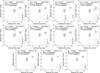 |
Fig. B.2. Fig. B.1 continued. |
| In the text | |
Current usage metrics show cumulative count of Article Views (full-text article views including HTML views, PDF and ePub downloads, according to the available data) and Abstracts Views on Vision4Press platform.
Data correspond to usage on the plateform after 2015. The current usage metrics is available 48-96 hours after online publication and is updated daily on week days.
Initial download of the metrics may take a while.