| Issue |
A&A
Volume 704, December 2025
|
|
|---|---|---|
| Article Number | A127 | |
| Number of page(s) | 10 | |
| Section | Astrophysical processes | |
| DOI | https://doi.org/10.1051/0004-6361/202556644 | |
| Published online | 03 December 2025 | |
The constraining power of X-ray polarimetry: Detailed structure of the intrabinary bow shock in Cygnus X-3
1
Department of Physics and Astronomy, FI-20014 University of Turku, Finland
2
Nordita, KTH Royal Institute of Technology and Stockholm University, Hannes Alfvéns väg 12, SE-10691 Stockholm, Sweden
⋆ Corresponding author: This email address is being protected from spambots. You need JavaScript enabled to view it.
Received:
29
July
2025
Accepted:
9
October
2025
Abstract
Context. Cygnus X-3 is the only known Galactic high-mass X-ray binary with a Wolf-Rayet companion. Recent X-ray polarimetry results with the Imaging X-ray Polarimetry Explorer have revealed it is a concealed ultraluminous X-ray source. It is also the first source for which pronounced orbital variability of X-ray polarization has been detected, notably with only one polarization maximum per orbit.
Aims. Polarization caused by scattering of the source X-rays can only be orbitally variable if the scattering angles change throughout the orbit. Since this requires an asymmetrically distributed medium around the compact object, the observed variability traces the intrabinary structures. The single-peaked profile further imposes constraints on the possible geometry of the surrounding medium. Therefore, the X-ray polarization of Cygnus X-3 offers an opportunity to study the wind structures of high-mass X-ray binaries in detail. We aim to uncover the underlying geometry through analytical modeling of the variable polarization. Knowledge of these structures could be extended to other sources with similar wind-binary interactions.
Methods. We studied the variability caused by single scattering in the intrabinary bow shock, exploring both the optically thin and optically thick limits. We considered two geometries for the reflecting medium: the axisymmetric parabolic bow shock and the parabolic cylinder shock. Finally, we determined which geometry offers the best match to the X-ray polarimetric data.
Results. Qualitatively, we find that the peculiar properties of the data can only be replicated with a cylindrical bow shock with asymmetry across the shock centerline and significant optical depth. This geometry is comparable to shocks formed by the jet-wind or outflow-wind interactions. In addition, the orbital axis is slightly misaligned from the observed orientation of the radio jet in all our model fits.
Key words: accretion / accretion disks / polarization / methods: analytical / X-rays: binaries
© The Authors 2025
 Open Access article, published by EDP Sciences, under the terms of the Creative Commons Attribution License (https://creativecommons.org/licenses/by/4.0), which permits unrestricted use, distribution, and reproduction in any medium, provided the original work is properly cited.
This article is published in open access under the Subscribe to Open model. This email address is being protected from spambots. You need JavaScript enabled to view it. to support open access publication.
1. Introduction
Cygnus X-3 (Cyg X-3) is a peculiar high mass X-ray binary (HMXB) with a Wolf-Rayet (WR) companion (van Kerkwijk et al. 1992). The compact object orbits through the dense WR wind, displaying infrared (IR) and X-ray orbital variability with a period of 4.8 hours (Becklin et al. 1973; Fender et al. 1999; Bonnet-Bidaud & van der Klis 1981). The system has a low inclination of about 30°, as measured through its orbital light curve (Antokhin et al. 2022) and spectrum (Vilhu et al. 2009) as well as its X-ray polarization (Veledina et al. 2024a,b). The inclination of its radio outflow was measured in Miller-Jones et al. (2004) at a lower value of ∼10°. The source features distinct X-ray spectral states that are correlated with its radio flux (Szostek et al. 2008). It is most frequently found in a hard X-ray, quiescent radio spectral state. It often transitions to an intermediate X-ray state, sometimes followed by an ultrasoft state and a soft nonthermal state, during which major radio ejections are observed. Although the spectrum of Cyg X-3 is close to typical hard and soft states in black hole X-ray binaries, it has strong Compton reflection-like features (Hjalmarsdotter et al. 2008, 2009; Koljonen et al. 2018). X-ray polarimetric observations with the Imaging X-ray Polarimetry Explorer (IXPE) (Weisskopf et al. 2022) found evidence of obscuring material close to the compact object (Veledina et al. 2024a). The average polarization degree (PD) of about 20% in the hard state and 10% in the intermediate and ultrasoft states (Veledina et al. 2024a,b) indicate the central source is concealed from view. This suggests that the compact object is surrounded by an optically thick toroidal outflow with a funnel-like cavity, which would be expected to form an ultraluminous X-ray source (King et al. 2001; Poutanen et al. 2007).
One unusual aspect of the X-ray polarization of Cyg X-3 is its significant orbital variability that remains consistent across spectral states. The PD varies by about 5% in all states, while the polarization angle (PA) varies by about 10° in the hard and intermediate states (Veledina et al. 2024a) and by 20° in the ultrasoft state (Veledina et al. 2024b). An orbital variability of the X-ray polarization has only been detected in two other sources: low-mass X-ray binary GS 1826−238 (Rankin et al. 2024) and the widely studied HMXB Cygnus X-1 (Cyg X-1, Kravtsov et al. 2025), both of which feature a much smaller amplitude compared to Cyg X-3. Interestingly, the PD and PA variations of both Cyg X-1 and Cyg X-3 exhibit only one peak per orbit. In Cyg X-3 in particular, the PD and PA peak at roughly the same orbital phase. Polarization caused by optically thin electron scattering from a corotating medium typically produces two peaks per orbit, unless significant asymmetry is present (Brown et al. 1978).
The orbital light curve of Cyg X-3 has one pronounced minimum, attributed to wind absorption at the superior conjunction (van der Klis & Bonnet-Bidaud 1981; van Kerkwijk 1993), along with smaller minima indicating the presence of one or more substructures in the WR wind (Vilhu et al. 2009; Antokhin et al. 2022). A secondary flux minimum preceding the inferior conjunction was explained by the presence of a “clumpy trail”, namely, a region of clumped gas caused by a jet bow shock colliding with the wind (Vilhu & Hannikainen 2013). The X-ray and infrared light curves were successfully modeled with three absorbing components: the wind, the clumpy trail, and the bow shock (Antokhin et al. 2022). All three components might potentially contribute to the polarization light curve as well. Scattering in the stellar wind will only have a minor effect on the polarization since it features an underlying spherical symmetry and multiple scatterings. The clumpy trail receives less flux than the bow shock and probably lacks the asymmetry required for producing single-peaked variability. This leaves the bow shock as the most likely primary cause of the orbital variability. An optically thick cylindrical bow shock was shown to be capable of producing the single-peaked variability at a qualitative level, although a quantitative fit was not found (Veledina et al. 2024a).
In this paper, we describe our development of the first model that is able to fit the orbital variability of X-ray polarization in Cyg X-3. We also discuss how we extracted useful parameters from the fit, including the shape of the bow shock. In Sect. 2, we introduce the equations for polarized single scattering and our model geometries. In Sect. 3, we present the model fits we carried out to compare the different geometries. In Sect. 4, we discuss the implications of our results and in Sect. 5, we provide a brief summary.
2. Model setup and data
2.1. Geometry
We represent linear polarization with the Stokes flux parameters FI, FQ, and FU. Using these parameters, the PD and PA can be obtained by  and tan2χ = FU/FQ, respectively. Stokes FQ and FU can also be expressed in their normalized form: q = FQ/FI and u = FU/FI. We assume that the compact object is in a counterclockwise circular orbit characterized by the orbital phase angle, φ, with φ = 0 corresponding to the superior conjunction. We used a corotating coordinate system fixed on the compact object, with the orbital axis,
  , aligned with the z-axis and the direction to the companion star aligned with the y-axis (see Fig. 1). In these coordinates, the direction toward the observer is
 (1)
(1)
where i is the observer inclination. The radial vector of a scattering point is
 (2)
(2)
where θ is the angle from the z-axis and ϕ is the azimuth measured from the x-axis. The cosine scattering angle is
 (3)
(3)
The normal of the scattering plane is the polarization pseudo-vector,
 (4)
(4)
The polarization angle depends on the choice of polarization basis; for this, we selected the projection of the orbital axis on the plane of the sky,
 (5)
(5)
 (6)
(6)
The PA of light scattered from point  (assuming the incident light is unpolarized) is
 (7)
(7)
 (8)
(8)
In reality, the projection of the orbital axis is misaligned from the north-south direction by its position angle, Ω (measured counterclockwise from the north). The observed q and u are related to the model via the rotation,
 (9)
(9)
 (10)
(10)
2.2. Polarized scattering
We define FI, 0(r, θ, ϕ),FQ, 0(r, θ, ϕ), and FU, 0(r, θ, ϕ) as the Stokes fluxes of radiation incident to an electron scattering envelope as a function of radial distance from the source, r, and the angles, θ and ϕ. Then, the Stokes vector of light scattered once by an optically thin envelope (Brown et al. 1978; Fox 1993) is
 (11)
(11)
where P(θ1, ϕ1, θ2, ϕ2) is the scattering matrix (Chandrasekhar 1960, pp. 40–42), σT is the Thomson cross-section, D is the distance to the observer, and n(r) is the electron number density of the envelope as a function of the radius vector, r. The first azimuthal angle of the scattering matrix is set to π/2 − φ so that its definition matches that of Chandrasekhar (1960). If the incident emission from the source is unpolarized and isotropic, the integral can be simplified to
 (12)
(12)
where L is the source luminosity. The integrand of Eq. (12) can be separated into components varying at the orbital frequency and its second harmonic,
 (13)
(13)
The orbital frequency components of two scattering points located at θ and π − θ have the same amplitude with opposite signs. Thus, scattering from any optically thin envelope that is symmetric relative to the x − y plane will only produce the second harmonic of the orbital frequency. This behavior is present even if the incident radiation is polarized or anisotropic as long as its angular distribution shares this symmetry.
For an optically thick surface with uniform scattering albedo λ, the single-scattered flux is
 (14)
(14)
where  is the cosine of the angle between the observer and the surface normal and
  is the cosine of the angle between the normal and the radial vector of the reflecting point. We treated the optically thick surface as fully opaque; the surface is only visible when η > 0 and η0 > 0. We note that we did not consider any self-obscuration of the shock.
The total flux is a combination of the shock scattering and direct radiation. This can be expressed in units of direct flux as
 (15)
(15)
where F0 and q0 represent a constant component. We only considered zero u0, which is expected from the constant component that is symmetric relative to the orbital plane.
2.3. Model for the incident light
We considered the case of incident flux from the reflecting funnel model described in Veledina et al. (2024a). In the model, unpolarized and isotropic incident radiation of the compact object with a flux of  is reflected off an optically thick truncated cone. To simplify the problem, we assumed that the point the light is reflected toward is located at a large distance, so the incident light is a point source for the scattering medium. The geometry is characterized by two parameters: the grazing angle of the cone, α, and the distance from the compact object to the outer edge of the cone, R. The observed average polarization of Cyg X-3 in its hard state is consistent with parameter values of α = 10° and R = 10 (in units of the truncated cone base radius; Veledina et al. 2024a). Thus, we used these values in our calculations to reduce the number of free parameters. We also combined the normalization parameters, including the constant flux, F0, the albedo of the cone, λcone, and the albedo of the shock, λshock, into one parameter: ϵ = λconeλshockF⋆/F0.
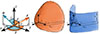 |
Fig. 1. Illustration of the coordinate system used in this work (left) and sketches of the parabolic (center) and parabolic cylinder (right) shock geometries. |
Figure 2 shows FI, 0/F⋆ and FQ, 0/FI, 0 as a function of the colatitude, θ, with the single-scattering albedo set to unity. At angles θ < α, the direct radiation from the central source is visible, and the total flux is about 20 times greater than the reflected alone. With a more realistic single-scattering albedo of λ ∼ 0.1 for neutral matter, the ratio between the reflected flux and the direct flux at θ ∼ 45° is only about 10−4. A highly ionized cone with multiple scatterings provides a similar ratio between the beamed flux and the reflection (Dauser et al. 2017). Due to the significant obscuration, we only considered cases where the region of the bow shock that reaches above the funnel is sufficiently rarefied that it gives only a minor contribution to the total scattered flux. Otherwise, scattering from gas directly above the funnel would dominate over all other regions, resulting in nearly constant (orbital phase-independent) polarization.
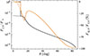 |
Fig. 2. Stokes FI, 0/F⋆ (black) and FQ, 0/FI, 0 (orange) of light reflected from the optically thick surface of a truncated cone as a function of the angle, θ. Dotted lines show the reflected light without direct radiation from the source. |
2.4. Scattering from a point-like cloud
We first considered the simple case where the shock is represented by a point scattering the incident radiation, located at a fixed colatitude, θ0, and azimuth, ϕ0. For unpolarized incident radiation, the reflected Stokes flux is
 (16)
(16)
where ϵ = fscF⋆/F0 is the flux normalization factor that includes the scattering fraction, fsc. This equation follows from Eq. (12) when the size of the scattering region is sufficiently small. This approach is similar to the phase-dependent polarization in the rotating vector model (used to explain the variable polarization of pulsars, Poutanen 2020; Meszaros et al. 1988; Radhakrishnan & Cooke 1969).
2.5. Parabolic bow shock
In an idealized case, a spherical object traveling through a medium will produce a parabolic bow shock. The geometry is illustrated in Fig. 1. Density at the shock boundary for an ideal strong bow shock is (DuPont et al. 2024)
 (17)
(17)
where nwr is the density of the Wolf-Rayet wind and γ is the adiabatic index. For the classical result of γ = 5/3, the shock is therefore four times as dense as the wind.
We set both the direction of orbital motion and the shock apex along the x-axis. To model a misaligned shock, the orbital phase angle can be shifted by the angle between the directions of the shock apex and the orbital motion. The shape of the parabolic bow shock is defined by the relation
 (18)
(18)
where a is the radius of the shock cross-section at x = 0 in units of distance to the shock apex. Due to the axial symmetry of the shock around x, it is easier to perform the calculations in rotated spherical coordinates measuring the colatitude angle with respect to the x-axis, cos ϑ = sin θcos ϕ, and the azimuthal angle from the y-axis toward the z-axis, tanψ = cos θ/(sin θ sin ϕ). We parameterized the extent of the shock by the maximal angle from the apex, ϑmax. The distance from the central source to the parabolic surface is
 (19)
(19)
and the normal to the surface of the paraboloid is
 (20)
(20)
To model an optically thin shock using the volume integral in Eq. (11), we treated the shock as a geometrically thin shell with constant column number density along r,
 (21)
(21)
This reduces Eq. (11) into a two-dimensional integral over ϑ and ψ at r = rp(ϑ). Using the same notation, we can write the surface element of the paraboloid for the optically thick integral in Eq. (14) as
 (22)
(22)
2.6. Cylindrical bow shock
To account for the potential modification of the shock shape caused by the jet-wind or funnel-wind interaction, we considered an alternative geometry for the shock as a sector of a parabolic cylinder as depicted in Fig. 1 (blue surface, Yoon & Heinz 2015; Yoon et al. 2016). With the apex along the x-axis, the cylinder is defined by the equation
 (23)
(23)
where a is the radius of the cylinder at x = 0 in units of distance to the shock apex. In the same units, we limit the height of the shock to |z|≤h. A misaligned shock can again be modeled by shifting the orbital phase angle. The maximal extent of the shock is defined by the azimuthal angle ϕmax. The cylindrical radius  of the shock surface is
 (24)
(24)
while the surface normal is
 (25)
(25)
The integral in Eq. (14) is most conveniently performed in cylindrical coordinates, where the surface element is
 (26)
(26)
2.7. Data analysis
We reanalyzed phase-resolved X-ray polarimetric data from IXPE (observation ID 02001899, first presented in Veledina et al. 2024a). The data were downloaded from the HEASARC public archive1 and processed with the IXPEOBSSIM package version 31.0.1 (Baldini et al. 2022) using the detector responses from CalDB version 13. The source photons were extracted from a circular region centered on the source, with a radius of 60″. The observation was folded with the quadratic ephemeris of Antokhin & Cherepashchuk (2019) using the xpphase method. The data were then grouped into ten phase bins and the pcube method was applied to each of the phase bins in the energy range of 3.5−6 keV. This energy range has little contribution from multiple scatterings or fluorescence, which would reduce the PD as compared to single scattering (Veledina et al. 2024a).
We employed the statistical modeling package Turing.jl, implementing the No-U-Turn sampler (Fjelde et al. 2025; Hoffman & Gelman 2014) to perform a Bayesian Markov chain Monte Carlo fitting of the data. This approach aims to find the posterior probability distributions of the model parameters with random sampling. We calculated the posterior likelihood of each sampled parameter set by comparing the model to the observed Stokes q and u, with the assumption that the data are distributed normally with a standard deviation equal to their error. To speed up calculation of our models that involve numeric integration, we precalculated them as parameter lookup tables and performed linear interpolation to find the results. We note that the statistically significant inference of all geometric parameters is unrealistic due to the low number of data points. Consequently, we fixed the inclination to i = 30° in all models, and fixed the parameters a and h whenever necessary. This introduces a systematic uncertainty to the inferred parameters, although the fitting procedure would indicate whether a particular shock geometry can replicate the observations. The specific inclination was chosen given its consistency with previously measured values (Antokhin et al. 2022; Vilhu et al. 2009; Miller-Jones et al. 2004) and we also found that varying it by ±10° did not significantly alter the parameters of the fit.
3. Results
3.1. Point-like scattering
We first applied the point-like single scattering model to the data. Scattering from a point-like cloud can only produce single-peaked orbital variability if it is elevated high above the orbital plane. This is shown in Eq. (13), where the orbital frequency component is ∝sin2θ0, whereas the second harmonic is ∝sin2θ0; therefore, the single-peaked variability can only dominate at small θ0 values. We assumed that the scattering point is above the funnel and receives the direct unpolarized emission from the central source. Since the phase of the superior conjunction is not necessarily the observed zero phase, we summed the phase shift and ϕ0 to create a new parameter, φ0. Thus, the model has five parameters in total: θ0, φ0, ϵ, Ω, and q0.
Figure 3 shows the best fit of the model, and the posterior distributions are shown in Fig. A.1. To quantify the quality of the fit, we calculated the Akaike information criterion (AIC) value and performed an Anderson-Darling (AD) test comparing the distribution of the normalized residuals to a standard normal distribution. The best fit has AIC = 104, with and AD p-value of 0.015. The point-like cloud fits the data only roughly given its mostly sinusoidal variability. This simple model cannot replicate the data in which the peaks of Stokes q and u appear near the same phase. The parameters q0 and ϵ are strongly degenerate in this case and neither can be constrained. The colatitude of the cloud,  (1σ), places it almost directly above the funnel. With the combined phase shift and azimuthal angle of φ0 = −106° ±11°, the cloud is located away from the companion star. The orbital axis is very closely aligned with the north-south direction, with a position angle of
  . We conclude that the point-like single scattering cloud cannot explain the observed variability, as the PD and PA maxima cannot appear near the same phase.
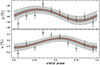 |
Fig. 3. Observed Stokes q and u of Cyg X-3 compared to the best fit of the point-like cloud model (dark red) and the 1- and 3-σ quantiles of the fit posterior (dark and light regions, respectively). |
3.2. Parabolic bow shock
The parabolic bow shock model suffers from the same shortcomings as the point-like cloud. Constant polarization dominates if the shock covers the funnel opening, and in the optically thin scenario, the axial symmetry would lead to the second harmonic dominating (two peaks per orbital period). Asymmetry can nevertheless be introduced by excluding the lower half of the shock, which can be interpreted as an accretion disk obscuring it from view. Figure 4 shows the reflected Stokes q and u for an optically thick shock and the upper half of an optically thin shock, with incident light from the funnel as described in Sect. 2.3. Even with the added vertical asymmetry, the variability in the optically thin case is dominated by the second harmonic. Hence, fully optically thin shock models are not capable of reproducing the data. This is a consequence of the narrow shock lying close to the orbital plane. Thus, the obscuration of the scattering surface would be necessary for the shock to produce only one polarization peak per orbit.
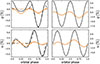 |
Fig. 4. Stokes q and u of a theoretical parabolic bow shock of width ϑmax = 30° (black) and ϑmax = 80° (orange) with a = 1 (solid) and a = 3 (dashed), for both the optically thick (left) and optically thin (right) cases. The flux was normalized so that the maximum of the scattered flux is one tenth of the direct flux. |
We proceeded to fit the optically thick parabolic shock to the data. The angle between the shock apex and the direction of motion is not separable from the phase shift of the observation, so we combined them into a single parameter, φ0. This leaves us with six parameters to fit: ϑmax, a, ϵ, Ω, φ0, and q0. The results of the fit are shown in Figs. 5 and A.2. With an AIC of 117 and an AD p-value of 0.0093, the fit is poor. The geometrical parameters a and ϑmax are degenerate with the flux normalization, ϵ, leading to a wide posterior distribution. The three remaining parameters are better constrained, with  matching the value of the point-like scattering model. The constant polarization
  is well within the error bars of the phase-average polarization in the 3.5−6 keV band, 22.8 ± 0.4% (Veledina et al. 2024a). The orientation of the shock
  is similar to the expected angle of about 35° (Antokhin et al. 2022).
3.3. Symmetric cylindrical bow shock
Next, we considered the cylindrical bow shock (Fig. 1, right). We assumed an optically thick shock with incident light coming from the cone reflection. We note that an optically thin cylindrical shock is similar to the parabolic bow shock with its mostly double-peaked variability. Since this model has too many parameters to infer from the data, we fixed the inclination to i = 30° and first performed a fit with a and h as free parameters. We then performed a second fit with the two parameters fixed to their best fitting values. Combining the phase shifts and fixing a and h, the model has five parameters to fit: ϕmax, ϵ, Ω, φ0, and q0.
The prior for h is limited by the elevation at which the direct radiation becomes visible to the shock (in units of distance to the shock apex), expressed as
 (27)
(27)
As this depends on a, we replaced h with the ratio h/hmax in the fit. Using uniform priors of 0.3−3.0 and 0.1−0.99 for a and h/hmax, respectively, the fit posterior was  and h/hmax = 0.6 ± 0.3 with best-fit values of a = 1.35 and h = 5.57.
Figure 6 shows the best fit of the model with fixed a and h, and the posterior distributions of its parameters are given in Fig. A.3. The best fit has an AIC value of 101 and an AD p-value of 0.037. Qualitatively, the model follows the observed Stokes u reasonably well but fits q poorly. This is a consequence of the symmetry of the shock relative to the x − z plane. When the apex of the shock is facing the observer and obscuring the reflecting inner surface, the observer only sees the constant component. The maxima of Stokes q occur before and after this plateau, while the symmetry of the shock leads to those peaks being identical. The observed Stokes q only has one clear maximum, which cannot be reproduced by this model.
The angle φ0 = 43° ±6° is again close to the expected value of ∼35°. With ϕmax = 66° ±7°, the shock is narrow. The constant component is highly constrained at q0 = −23.6 ± 0.4%, which is also consistent with the phase-averaged polarization. The flux normalization factor of  is large, corresponding to a peak reflected flux of about 0.3F0. The analytical model for cone scattering at i = 30° predicts a value of λconeF⋆/F0 ≈ 3 × 10², but this value for ϵ can be larger by nearly an order of magnitude if λshock is small. This can be explained by wind absorption toward the observer or the optically thick single-scattering model underestimating the reflected flux. The alignment angle of the orbital axis,
  , is consistent with that inferred from the point-like cloud model.
3.4. Asymmetric cylindrical bow shock
We further tested the parabolic cylinder geometry by adding asymmetry across the shock centerline. In a more accurate model, the shock curves into a spiral shape as it collides with the wind. However, this is a difficult geometry to model analytically. Thus, to explore the impact of this asymmetry, we separated widths of the shock on either side of the shock apex into free parameters. Firstly, ϕmax1 is the width of the shock away from the companion (negative y-direction), and, secondly, ϕmax2 is the width toward the companion (positive y-direction). As with the symmetric shock, we fixed the inclination to i = 30° and performed an initial fit including a and h/hmax as free parameters. The fit results were  and
and  , with the best-fit values of a = 1.63 and h = 3.35. The results of the second fit with fixed a and h can be seen in Figs. 7 and A.4. The best fit gives AIC = 78 and an AD p-value of 0.61.
We find that the model replicates the single peaks of q and u that occur roughly at the same phase. The model fit has by far the best AIC value and is the only one where the AD test does not reject the null hypothesis of Gaussian residuals. The qualitative difference is easier to visualize in the q − u plane shown in Fig. 8, where the data trace a narrow, skewed shape. Out of the three model fits, the asymmetric cylinder shock is the only one capable of reproducing the data topology. However, this model exhibits constant polarization over a relatively large portion of the orbit and, thus, it does not aptly fit the polarization near phase zero.
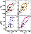 |
Fig. 8. Observed variability in the q − u plane compared to the best fits of the point-like cloud (top left), parabolic shock (top right), symmetric cylinder shock (bottom left), and the asymmetric cylinder shock (bottom right). |
Interestingly, the two widths of the shock are starkly different, with the fit preferring a larger angle  for one side and a much smaller angle
  for the other. The angle
  places the apex of the shock facing the companion star. With these parameters, the shock is practically a curved wall facing toward the direction of orbital motion with a small “hook” on the other side of the apex (see magenta shape in Fig. 9). This makes the reflection only visible around phase 0.5.
 |
Fig. 9. Illustration of how the best fit of the asymmetric cylinder shock (magenta) compares to a shock curved by the wind (cyan). |
The constant polarization is again strongly constrained at q0 = −24.2 ± 0.4%, which is about 2σ higher than the average polarization. The flux normalization of  is larger than the symmetric model, although the reflected flux is similar due to the reduced shock height, peaking at 0.4F0. The position angle
  is again consistent with the constraints from the other three models.
4. Discussion
4.1. Properties of the shock
The geometry of the intrabinary bow shock in Cyg X-3 is strongly constrained by the X-ray polarimetric data. If the shock is the primary cause of the orbitally variable polarization and sufficiently represented by our model, it must be both cylindrical and asymmetric with regard to the shock apex. This is consistent with theoretical predictions of the bow shock shape in simulations, as the tail of the shock is expected to curve under orbital motion (Eichler & Usov 1993). Figure 9 shows how this shape compares to the best fit of our model. The simplified asymmetric shock is roughly analogous to the curving shock, with the narrow  corresponding to the convex part of the shock. The surface of this convex side would not be exposed to the central source far from the shock apex, so the extent of the shock surface would appear narrower on that side. However, the much wider
  does not match the concave half of the curving shock far away from the apex. A more physical model would include the geometric thickness of the shock, its density distribution, its curvature further away from the shock apex, and multiple scatterings; however, this is beyond the scope of this work. Nevertheless, models with many scatterings may face problems explaining the prominent variability as the amplitude would be reduced.
The polarized variability having one peak per orbit can only be recreated if the shock scattering is obscured during certain orbital periods. Therefore, the shock must be at least moderately optically thick. Our simplified model uses an infinite optical depth and thus cannot constrain the optical depth of the shock. A model fit of an axisymmetric bow shock in Antokhin et al. (2022) determined the shock optical depth through the apex as ∼1.1, with the maximum optical depth through the line of sight being ∼0.6. Our conclusion that the shock is opaque enough to obscure its inner surface could be consistent with this model if the shock is denser at lower elevations.
We examined the orbital variability only in the hard state, yet it is present in all observations. The ultrasoft and intermediate states have a smaller constant PD that can be explained with scattering from an optically thin medium above the funnel (Veledina et al. 2024b). In this scenario, the primary source of X-rays incident on the shock would be the scattered flux, rather than the cone reflection. Furthermore, the radio jet is quenched in the ultrasoft state, which can impact the shock geometry. These differences likely explain the changes in the orbital variability of polarization. Even so, the persistent single-peaked profile makes a semi-stable source for the variability a necessity. Therefore, the vertically extended shock has to be sustained by the outflow-wind interaction if the jet is absent.
4.2. Alignment of the orbital axis and the jet
The only parameter that remained consistent throughout all our model fits was the small positive value of the position angle, Ω. Although the small rotation has little impact on q, it shifts u toward negative values. If the average value of u is slightly negative, it is reasonable to expect fits of different models to find similar values for the position angle. The near north-south alignment of the orbital axis is consistent with radio observations of the jet (Martí et al. 2000; Miller-Jones et al. 2004; Yang et al. 2023). Yang et al. (2023) measured the position angle of the innermost radio jet as  , which differs from our inferred value of
  by at least 5σ. While the result is model-dependent, it hints at a small misalignment of the jet with the orbital axis at the scale of the radio observations.
We did not account for a possibly inclined jet and outflow. However, the orbital gamma-ray variability and certain radio observations can be explained with an inclined and precessing jet (Dubus et al. 2010). The variability can also be explained by a jet bent by the wind, so the inclined jet cannot be confirmed nor rejected (Dmytriiev et al. 2024). The misalignment found by our analysis is significantly smaller than the ∼40° jet inclination or bending angle indicated by the gamma ray model fits. It is more in line with the predicted small bending angle that, however, depends on poorly defined jet parameters (Dmytriiev et al. 2024). The effects of an inclined jet on the orbital variability would be very complicated, as it introduces an orbital phase dependency on the jet-wind interaction (Yoon & Heinz 2015). Therefore, this analysis is beyond the scope of this work.
4.3. Impact of other wind structures
Scattering in the Wolf-Rayet wind contributes to the total observed polarization. With a spherically symmetric wind, the polarized flux would be nearly constant, yet the wind is warped by the gravity and the jet-wind interaction. However, the optically thin wind would primarily produce two PD and PA peaks per orbit and thus cannot be a dominant component in the observed variability (Veledina et al. 2024a). It might still contribute to the constant Stokes q0, which would be difficult to separate from the constant component caused by the funnel reflection. Inferring the geometrical parameters of the funnel could be more complicated if the constant polarization is indeed a sum of multiple components. It is difficult to estimate the contribution from the wind, but simulations of single-scattering in the HMXB wind at lower wind mass loss rates than Cyg X-3 show negligible polarized flux outside of eclipses (Kallman et al. 2015). The higher wind density of Cyg X-3 would lead to more pronounced wind scattering component contribution to the total flux, but the presence of multiple scatterings would decrease the PD.
Previous works analyzing the X-ray light curves of Cyg X-3 have assumed a constant initial flux that is modulated at the orbital period by absorption at multiple wind structures (e.g., Vilhu & Hannikainen 2013; Antokhin et al. 2022). This analysis has neglected the contribution of a variable flux caused by scattering. Since strong orbital variability of polarization requires that a sizable fraction of the flux is scattered, the light curve should be revisited within this new context.
The variable flux from scattering cannot explain the light curve without absorption and, thus, a combination of scattering and absorption models is needed. The amount of reflected flux in the parabolic cylinder model is strongly dependent on both h and a, whereas neither parameter is well constrained. Nevertheless, we matched the IXPE light curve by combining the best fit of the asymmetric cylindrical bow shock and the absorption models of Antokhin et al. (2022). The large parameter space makes it impractical to obtain a statistically meaningful fit, so we only tested the model heuristically. We fixed the inclination to i = 30° and the radius of the WR star to one-third of the orbital separation. The results of our manual fitting are shown in Fig. 10. Using the parameter definitions of the aforementioned paper, we used wind absorption with τ0 = 0.33 and ϕ0 = −0.005, and two clump absorbers with τct, 1 = 0.41, τct, 2 = 0.31, ϕct, 1 = 0.475, ϕct, 2 = 0.70, Δϕct, 1 = 0.274, and Δϕct, 2 = 0.20. The two absorbers occur before and after the peak of the reflected flux and, in the context of this manual fit, they can be interpreted as absorption in the curving tails of the bow shock (see Fig. 9). Absorption in the bow shock itself is not needed in the fit, perhaps because our model already has reduced normalized flux when the shock apex is facing the observer. Hence, the dimming due to absorption is degenerate with the enhancement of flux due to scattering from the inner surface of the shock. While this model gives the essence of the observed flux variability, a detailed study of the parameter space would be meaningful for the combined set of X-ray and IR light curves, similarly to the analysis presented in Antokhin et al. (2022).
 |
Fig. 10. Normalized IXPE orbital light curve of Cyg X-3 in the 3.5−6 keV range (black line) with the raw reflected flux from the best-fit asymmetric cylinder shock model (magenta dashed line) and a hand-fitted model light curve, with wind and clump absorption applied to the reflected flux (magenta solid line). |
Our assumption that the gas above the outflow must have negligible optical depth is complicated by the jet-wind interaction. Specifically, the wind causes the jet to curve and so, the bow shock would eventually reach above the funnel. The jet in Cyg X-3 is not strongly bent until a recollimation shock forms about one orbital separation above the orbital plane (Yoon et al. 2016). This is several orders of magnitude more distant from the source than the shock apex, so the scattered flux from the lower shock would at least be comparable to the scattered flux from high above. Assuming that the wind density decreases away from the WR star with the inverse square of distance, the wind near the recollimation shock would thus be about half as dense as the wind near the compact object. The part of the bow shock exposed to the direct radiation is therefore significantly less dense than the lower parts of the shock. All things considered, it is safe to conclude that scattering from the bow shock far above the outflow does not dominate.
4.4. Comparison with Cyg X-1
Similar bow shock structures should be present in other HMXBs, yet Cyg X-3 remains the only one with pronounced orbital X-ray polarization. In particular, Cyg X-1 is another wind-fed microquasar that was observed with IXPE, but the initial analysis by Krawczynski et al. (2022) found no statistically significant orbital variability. A subsequent analysis of the large set of observations showed that orbital variability with a single polarization maximum per orbit is present in Cyg X-1, albeit with PD amplitude of ∼2% (Kravtsov et al. 2025). The lower statistics of the orbital phase resolved polarization makes Cyg X-1 challenging for detailed study of its bow shock structure. The q and u maxima of Cyg X-1 occur at different orbital phases, which is expected from scattering of unpolarized radiation by an optically thin medium as demonstrated by Eq. (13). This variability could correspond to a bow shock that reaches above the orbital plane with its lower half obscured by the accretion disk, but we refrain from drawing further conclusions from the data due to their low statistics.
Cyg X-3 may have more significant variability due to its higher wind mass-loss rate, which was estimated by Antokhin et al. (2022) as ∼10−5 M⊙ yr−1, compared to 5 × 10⁻⁷ M⊙ yr−1 in Cyg X-1 (Ramachandran et al. 2025). The mass loss rate of Cyg X-1 was previously estimated by Gies et al. (2003) to be an order of magnitude larger with the further expectation that the wind is directed toward the compact object (Gies & Bolton 1986). Recently, Ramachandran et al. (2025) introduced a more comprehensive model with wind clumping and found no evidence for focused wind. Clumping and wind asymmetry were not considered in Antokhin et al. (2022), so the mass loss rate of Cyg X-3 may also be overestimated. It is accordingly difficult to estimate the density of the wind structures near either compact object, although the similarities in their orbital variability suggest that they might be roughly comparable. Cyg X-3 is the only known HMXB with a WR donor in our Galaxy, so it might be the only easily observable source with pronounced orbital variability of X-ray polarization. The opportunity to study the shock geometry in such detail is hitherto unique to Cyg X-3, making it a valuable tool in furthering our understanding of HMXB wind structures.
5. Summary
In this work, we have developed several analytical models for single scattering in the intrabinary bow shock in Cyg X-3 and compared their predictions with the X-ray polarization data. The only shock model we found capable of replicating the observed orbital variability is cylindrical, asymmetric across the shock apex, and optically thick. The single-peaked orbital variability strongly constrained the possible geometries. Scenarios with the medium located directly above the obscuring funnel face difficulties in terms of explaining the high amplitude of the variations, since most of the scattered flux would have a constant polarization. At the same time, any optically thin shock lying low on the orbital plane would lead to primarily two polarization peaks per orbit. Thus, the observed coincidence of the maxima in q and u Stokes parameters could only be achieved, in the framework of these models, if the shock has asymmetry relative to its centerline.
The inferred shape of the bow shock confirms the shock geometry predicted by simulations of the HMXB jet-wind interaction. The position angle of the orbital axis in our model fits deviates from the alignment of the innermost radio jet by a few degrees, which is consistent with an otherwise aligned jet with wind-induced bending. As the nature of the variability does not change even when the jet is quenched, the funnel outflow must be key in forming the shock geometry. Determining the exact properties of the shock and the impact of an inclined or curved jet would require more complex numerical modeling.
The high amplitude of the observed variability implies that the bow shock scattering is a significant fraction of the observed flux. Previous models for the orbital light curve should therefore be revised with the addition of a variable component to the unabsorbed flux. We have made a manual fit to the light curves and found that they can be explained by adding wind and clump absorption to the variable flux of our best-fit model. Therefore, we expect that estimates of the system’s basic parameters, such as its inclination, might change once the additional scattered flux is taken into account in the light curve modeling.
Acknowledgments
We thank Juri Poutanen and the anonymous referee for comments that greatly improved the manuscript. This work has been supported by a grant from the Turku University Foundation (VA). AV acknowledges support from the Academy of Finland grant 355672. Nordita is supported in part by NordForsk.
References
- Antokhin, I. I., & Cherepashchuk, A. M. 2019, ApJ, 871, 244 [Google Scholar]
- Antokhin, I. I., Cherepashchuk, A. M., Antokhina, E. A., & Tatarnikov, A. M. 2022, ApJ, 926, 123 [NASA ADS] [CrossRef] [Google Scholar]
- Baldini, L., Bucciantini, N., Lalla, N. D., et al. 2022, SoftwareX, 19, 101194 [NASA ADS] [CrossRef] [Google Scholar]
- Becklin, E. E., Neugebauer, G., Hawkins, F. J., et al. 1973, Nature, 245, 302 [Google Scholar]
- Bonnet-Bidaud, J. M., & van der Klis, M. 1981, A&A, 101, 299 [NASA ADS] [Google Scholar]
- Brown, J. C., McLean, I. S., & Emslie, A. G. 1978, A&A, 68, 415 [NASA ADS] [Google Scholar]
- Chandrasekhar, S. 1960, Radiative Transfer (New York: Dover) [Google Scholar]
- Dauser, T., Middleton, M., & Wilms, J. 2017, MNRAS, 466, 2236 [Google Scholar]
- Dmytriiev, A., Zdziarski, A. A., Malyshev, D., Bosch-Ramon, V., & Chernyakova, M. 2024, ApJ, 972, 85 [Google Scholar]
- Dubus, G., Cerutti, B., & Henri, G. 2010, MNRAS, 404, L55 [NASA ADS] [Google Scholar]
- DuPont, M., Gruzinov, A., & MacFadyen, A. 2024, ApJ, 971, 34 [Google Scholar]
- Eichler, D., & Usov, V. 1993, ApJ, 402, 271 [Google Scholar]
- Fender, R. P., Hanson, M. M., & Pooley, G. G. 1999, MNRAS, 308, 473 [NASA ADS] [CrossRef] [Google Scholar]
- Fjelde, T. E., Xu, K., Widmann, D., et al. 2025, ACM Trans. Probab. Mach. Learn., 1, 14 [Google Scholar]
- Fox, G. K. 1993, MNRAS, 260, 513 [Google Scholar]
- Gies, D. R., & Bolton, C. T. 1986, ApJ, 304, 389 [NASA ADS] [CrossRef] [Google Scholar]
- Gies, D. R., Bolton, C. T., Thomson, J. R., et al. 2003, ApJ, 583, 424 [Google Scholar]
- Hjalmarsdotter, L., Zdziarski, A. A., Larsson, S., et al. 2008, MNRAS, 384, 278 [NASA ADS] [CrossRef] [Google Scholar]
- Hjalmarsdotter, L., Zdziarski, A. A., Szostek, A., & Hannikainen, D. C. 2009, MNRAS, 392, 251 [NASA ADS] [CrossRef] [Google Scholar]
- Hoffman, M. D., & Gelman, A. 2014, J. Mach. Learn. Res., 15, 1593 [Google Scholar]
- Kallman, T., Dorodnitsyn, A., & Blondin, J. 2015, ApJ, 815, 53 [NASA ADS] [CrossRef] [Google Scholar]
- King, A. R., Davies, M. B., Ward, M. J., Fabbiano, G., & Elvis, M. 2001, ApJ, 552, L109 [NASA ADS] [CrossRef] [Google Scholar]
- Koljonen, K. I. I., Maccarone, T., McCollough, M. L., et al. 2018, A&A, 612, A27 [NASA ADS] [CrossRef] [EDP Sciences] [Google Scholar]
- Kravtsov, V., Bocharova, A., Veledina, A., et al. 2025, A&A, 701, A115 [NASA ADS] [CrossRef] [EDP Sciences] [Google Scholar]
- Krawczynski, H., Muleri, F., Dovčiak, M., et al. 2022, Science, 378, 650 [NASA ADS] [CrossRef] [Google Scholar]
- Martí, J., Paredes, J. M., & Peracaula, M. 2000, ApJ, 545, 939 [Google Scholar]
- Meszaros, P., Novick, R., Szentgyorgyi, A., Chanan, G. A., & Weisskopf, M. C. 1988, ApJ, 324, 1056 [NASA ADS] [CrossRef] [Google Scholar]
- Miller-Jones, J. C. A., Blundell, K. M., Rupen, M. P., et al. 2004, ApJ, 600, 368 [NASA ADS] [CrossRef] [Google Scholar]
- Poutanen, J. 2020, A&A, 641, A166 [NASA ADS] [CrossRef] [EDP Sciences] [Google Scholar]
- Poutanen, J., Lipunova, G., Fabrika, S., Butkevich, A. G., & Abolmasov, P. 2007, MNRAS, 377, 1187 [NASA ADS] [CrossRef] [Google Scholar]
- Radhakrishnan, V., & Cooke, D. J. 1969, Astrophys. Lett., 3, 225 [NASA ADS] [Google Scholar]
- Ramachandran, V., Sander, A. A. C., Oskinova, L. M., et al. 2025, A&A, 698, A37 [NASA ADS] [CrossRef] [EDP Sciences] [Google Scholar]
- Rankin, J., Kravtsov, V., Muleri, F., et al. 2024, ApJ, 962, 34 [NASA ADS] [CrossRef] [Google Scholar]
- Szostek, A., Zdziarski, A. A., & McCollough, M. L. 2008, MNRAS, 388, 1001 [NASA ADS] [Google Scholar]
- van der Klis, M., & Bonnet-Bidaud, J. M. 1981, A&A, 95, L5 [NASA ADS] [Google Scholar]
- van Kerkwijk, M. H. 1993, A&A, 276, L9 [NASA ADS] [Google Scholar]
- van Kerkwijk, M. H., Charles, P. A., Geballe, T. R., et al. 1992, Nature, 355, 703 [NASA ADS] [CrossRef] [Google Scholar]
- Veledina, A., Muleri, F., Poutanen, J., et al. 2024a, Nat. Astron., 8, 1031 [NASA ADS] [CrossRef] [Google Scholar]
- Veledina, A., Poutanen, J., Bocharova, A., et al. 2024b, A&A, 688, L27 [NASA ADS] [CrossRef] [EDP Sciences] [Google Scholar]
- Vilhu, O., & Hannikainen, D. C. 2013, A&A, 550, A48 [NASA ADS] [CrossRef] [EDP Sciences] [Google Scholar]
- Vilhu, O., Hakala, P., Hannikainen, D. C., McCollough, M., & Koljonen, K. 2009, A&A, 501, 679 [NASA ADS] [CrossRef] [EDP Sciences] [Google Scholar]
- Weisskopf, M. C., Soffitta, P., Baldini, L., et al. 2022, JATIS, 8, 026002 [NASA ADS] [Google Scholar]
- Yang, J., García, F., del Palacio, S., et al. 2023, MNRAS, 526, L1 [Google Scholar]
- Yoon, D., & Heinz, S. 2015, ApJ, 801, 55 [NASA ADS] [CrossRef] [Google Scholar]
- Yoon, D., Zdziarski, A. A., & Heinz, S. 2016, MNRAS, 456, 3638 [NASA ADS] [CrossRef] [Google Scholar]
Appendix A: Plots of posterior distributions
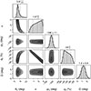 |
Fig. A.1. Posterior distribution of the point-like cloud model fit. |
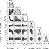 |
Fig. A.2. Posterior distribution of the parabolic shock model fit. |
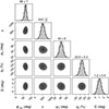 |
Fig. A.3. Posterior distribution of the symmetric parabolic cylinder shock model fit. |
 |
Fig. A.4. Posterior distribution of the asymmetric parabolic cylinder shock model fit. |
All Figures
|
Fig. 1. Illustration of the coordinate system used in this work (left) and sketches of the parabolic (center) and parabolic cylinder (right) shock geometries. |
| In the text | |
|
Fig. 2. Stokes FI, 0/F⋆ (black) and FQ, 0/FI, 0 (orange) of light reflected from the optically thick surface of a truncated cone as a function of the angle, θ. Dotted lines show the reflected light without direct radiation from the source. |
| In the text | |
|
Fig. 3. Observed Stokes q and u of Cyg X-3 compared to the best fit of the point-like cloud model (dark red) and the 1- and 3-σ quantiles of the fit posterior (dark and light regions, respectively). |
| In the text | |
|
Fig. 4. Stokes q and u of a theoretical parabolic bow shock of width ϑmax = 30° (black) and ϑmax = 80° (orange) with a = 1 (solid) and a = 3 (dashed), for both the optically thick (left) and optically thin (right) cases. The flux was normalized so that the maximum of the scattered flux is one tenth of the direct flux. |
| In the text | |
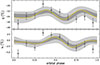 |
Fig. 5. Same as Fig. 3, but for the parabolic shock model. |
| In the text | |
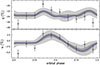 |
Fig. 6. Same as Fig. 3, but for the parabolic cylinder shock model. |
| In the text | |
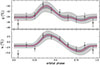 |
Fig. 7. Same as Fig. 3, but for the asymmetric parabolic cylinder shock model. |
| In the text | |
|
Fig. 8. Observed variability in the q − u plane compared to the best fits of the point-like cloud (top left), parabolic shock (top right), symmetric cylinder shock (bottom left), and the asymmetric cylinder shock (bottom right). |
| In the text | |
|
Fig. 9. Illustration of how the best fit of the asymmetric cylinder shock (magenta) compares to a shock curved by the wind (cyan). |
| In the text | |
|
Fig. 10. Normalized IXPE orbital light curve of Cyg X-3 in the 3.5−6 keV range (black line) with the raw reflected flux from the best-fit asymmetric cylinder shock model (magenta dashed line) and a hand-fitted model light curve, with wind and clump absorption applied to the reflected flux (magenta solid line). |
| In the text | |
|
Fig. A.1. Posterior distribution of the point-like cloud model fit. |
| In the text | |
|
Fig. A.2. Posterior distribution of the parabolic shock model fit. |
| In the text | |
|
Fig. A.3. Posterior distribution of the symmetric parabolic cylinder shock model fit. |
| In the text | |
|
Fig. A.4. Posterior distribution of the asymmetric parabolic cylinder shock model fit. |
| In the text | |
Current usage metrics show cumulative count of Article Views (full-text article views including HTML views, PDF and ePub downloads, according to the available data) and Abstracts Views on Vision4Press platform.
Data correspond to usage on the plateform after 2015. The current usage metrics is available 48-96 hours after online publication and is updated daily on week days.
Initial download of the metrics may take a while.