| Issue |
A&A
Volume 704, December 2025
|
|
|---|---|---|
| Article Number | A311 | |
| Number of page(s) | 6 | |
| Section | Extragalactic astronomy | |
| DOI | https://doi.org/10.1051/0004-6361/202557558 | |
| Published online | 18 December 2025 | |
Intra-night optical polarization monitoring of blazars
1
Department of Physics, University of Crete, GR-70013 Heraklion, Greece
2
Institute of Astrophysics, Foundation for Research and Technology-Hellas, Vasilika Vouton, GR-70013 Heraklion, Greece
3
Institute for Astrophysical Research, Boston University, 725 Commonwealth Avenue, Boston, MA 02215, USA
4
Saint Petersburg State University, 7/9 Universitetskaya nab., St. Petersburg 199034, Russia
5
Instituto de Astrofísica de Andalucía, IAA-CSIC, Glorieta de la Astronomía s/n, 18008 Granada, Spain
6
Aix Marseille Univ, CNRS, CNES, LAM, Marseille, France
7
Department of Space, Earth and Environment, Chalmers University of Technology, Gothenburg, Sweden
8
Dr. Karl Remeis-Observatory and Erlangen Centre for Astroparticle Physics, Friedrich-Alexander Universität Erlangen-Nürnberg, Sternwartstr. 7, 96049 Bamberg, Germany
9
INAF Osservatorio Astronomico di Brera, Via E. Bianchi 46, 23807 Merate (LC), Italy
10
Center for Astrophysics | Harvard & Smithsonian, 60 Garden Street, Cambridge, MA 02138, USA
11
Istituto Nazionale di Fisica Nucleare, Sezione di Padova, 35131 Padova, Italy
12
Department of Physics and Astronomy, University of Turku FI-20014, Finland
★ Corresponding authors: This email address is being protected from spambots. You need JavaScript enabled to view it.
; This email address is being protected from spambots. You need JavaScript enabled to view it.
Received:
4
October
2025
Accepted:
12
November
2025
Abstract
Blazars are known for their extreme variability across the electromagnetic spectrum. Variability at very short timescales can allow us to discriminate between competing models. This is particularly true for polarization variability, which allows us to probe particle acceleration and high-energy emission models in blazars. Here we present results from the first pilot study of intra-night optical polarization monitoring conducted using RoboPol at the Skinakas Observatory; these results are supplemented by observations from the Calar Alto, Perkins, and Sierra Nevada observatories. Our results show that while variability patterns can vary widely between sources, variability on timescales as short as minutes is prevalent in blazar jets. The amplitudes of the variations are typically small, a few percent for the polarization degree and less than 20° for the polarization angle, pointing to a significant contribution to the optical emission from a turbulent magnetic field component. The overall stability of the polarization angle over time points to a preferred magnetic field orientation.
Key words: polarization / relativistic processes / galaxies: active / BL Lacertae objects: general / galaxies: jets
© The Authors 2025
 Open Access article, published by EDP Sciences, under the terms of the Creative Commons Attribution License (https://creativecommons.org/licenses/by/4.0), which permits unrestricted use, distribution, and reproduction in any medium, provided the original work is properly cited.
This article is published in open access under the Subscribe to Open model. This email address is being protected from spambots. You need JavaScript enabled to view it. to support open access publication.
1. Introduction
Blazars are the brightest active galactic nuclei due to the preferential alignment of their jets toward Earth (Blandford et al. 2019; Hovatta & Lindfors 2019). On timescales of decades, their multiwavelength emission spans from the lowest radio frequencies to the very high-energy γ-rays. Their spectral energy distribution is typically characterized by two broad emission components (often referred to as humps) intersecting in the eV-MeV range depending on the spectral subclass. The first hump is due to synchrotron radiation, while the second is thought to originate from either Compton scattering of relativistic electrons or emission from relativistic protons, with recent observations favoring the former over the latter (Agudo et al. 2025; Liodakis et al. 2025). The spectral subclasses in blazars are defined according to the location of the synchrotron peak as low- (LSP; < 1014 Hz), intermediate- (1014–1015 Hz), and high- (HSP; > 1015 Hz) synchrotron peaked sources (Ajello et al. 2020).
The origin of the particle acceleration happening in the jets and the origin of the high-energy emission (second hump) are still a matter of debate, though a lot of progress has been made in the past few years (e.g., Di Gesu et al. 2023; Peirson et al. 2023; Middei et al. 2023; Marshall et al. 2024). Polarization variability can be a powerful tool for differentiating between different models. In 2013 the RoboPol survey was launched at the Skinakas observatory in Crete to uncover the relation of polarization variability to γ-ray emission (Blinov et al. 2015, 2018, 2021). The program ran from 2013 to 2017, observing a large number of blazars with regular, few-day cadences. The RoboPol survey was able to triple the number of known Electric Vector Position Angle (EVPA) rotations (Blinov et al. 2015, 2016a,b) and demonstrate their connection to γ-ray flares (Blinov et al. 2018), as well as uncover the anticorrelation between polarization degree and synchrotron peak, predicting the energy stratification of the electrons (Angelakis et al. 2016) that was later confirmed by X-ray polarization observations of HSP sources (e.g., Liodakis et al. 2022; Di Gesu et al. 2022; Kouch et al. 2024).
However, in their analysis they found that the nominal few-day cadence of the survey was likely under-sampling the light curves, resulting in the masking of fast electron vector position angle rotations (Kiehlmann et al. 2021). Such rotations can be very important in differentiating between particle acceleration mechanisms (e.g., Liodakis et al. 2024). Intra-night variability of the total intensity has been studied in several blazars (e.g., Sagar et al. 2004; Goyal et al. 2012; Bachev et al. 2012; Negi et al. 2023; Agarwal et al. 2023; McCall et al. 2024); however, intra-night polarization variability studies have been limited to a few selected objects (e.g., Villforth et al. 2009; Fraija et al. 2017; Bachev et al. 2023; Liodakis et al. 2024).
Building on the previous RoboPol results, as well as recent findings of the Imaging X-ray Polarimetry Explorer (Chen et al. 2024; Marscher et al. 2024; Capecchiacci et al. 2025), we conducted a pilot survey from 2024 to early 2025 to uncover intra-night variable sources in polarization that could potentially show these very fast polarization angle rotations. In Sect. 2 we discuss the sample selection and analysis. In Sect. 3 we present the results from the pilot survey and a comparison with the previous RoboPol monitoring. In Sect. 4 we present our conclusions.
2. Sample and analysis
Our sample is a subset of the statistically complete RoboPol survey sample of γ-ray-loud blazars (Pavlidou et al. 2014; Blinov et al. 2021). From the original sample, we selected all LSP sources with a GaiaG-band magnitude brighter than 16.5. This resulted in the 20 sources listed in Table 1.
Polarization and variability properties for the sources included in this study.
The analysis of the observations was done using the semiautomatic RoboPol pipeline. Details can be found in King et al. (2014), Panopoulou et al. (2015), and Blinov et al. (2021). The observations were corrected for instrumental polarization and angle rotation using unpolarized and polarized standard stars (Blinov et al. 2023). The standard stars were observed every night and then averaged over several nights to achieve a better characterization of the instrumental polarization. The individual observing times for the sources in the sample vary based on the previous RoboPol observations. For the analysis presented here, to achieve a > 3σ detection of the polarization degree, adjacent exposures were adaptively binned to maximize the signal-to-noise while maintaining a high cadence. We started by binning two adjacent data points and evaluated if the number of upper limits in the light curve was significantly reduced. If not, we repeated the procedure for three adjacent data points. The binning was applied only to individual nights and not the entire dataset for a given source. This process was only applied to four sources, namely J1512-0905, J1800+7828, J2143+1743, and J2148+0657.
We supplemented our RoboPol observations with data taken in 2024–2025 as part of the Boston University BEAM-ME1 program (Marscher & Jorstad 2021) and the Calar Alto and Sierra Nevada Observatory (SNO) blazar monitoring program (Agudo et al. 2012; Otero-Santos et al. 2024). BEAM-ME uses the 1.8 m telescope of the Perkins Observatory (Flagstaff, AZ, USA), and the PRISM polarimeter. The Calar Alto and SNO observations were taken using Calar Alto Faint Object Spectrograph (CAFOS) and DIPOL-1, respectively, and were analyzed with the IOP4 pipeline described in Escudero Pedrosa et al. (2024a,b). The additional observations were typically carried out within a few days of the RoboPol observations. For J1058+5628 we were only able to obtain one night of observations using the Perkins telescope. The polarization degree was de-biased following Blinov et al. (2021). The contribution of the interstellar polarization for the sources in our sample is typically < 1%, and any depolarization from the host galaxy for LSP sources is typically negligible. Regardless, since we are interested in identifying variability, our results should not be affected by either effect. All the raw measurements of the Stokes parameters from our pilot survey without any quality cuts, corrections, or binning are available in the Harvard dataverse2.
In total, we obtained 65 nights of observations for the entire sample (see Table 1) with varying lengths due to observing conditions and seasonal night-length variations. We were able to achieve a median cadence of a few minutes, typically < 7 minutes, with a minimum of 1.5 minutes (Table 1).
To assess whether the sources exhibit intra-night variability, we needed to define a variability metric. We attempted a simple chi-square approach of comparing the observed data for each night against a constant value; however, such an approach suffers in two ways. First, it is highly sensitive to outliers, and second, it is not trivial to define an appropriate threshold to differentiate variable from non-variable light curves. For that reason, we partially adopted the methodology proposed by Sokolovsky et al. (2017), who compared the performance of various variability detection techniques in photometric time series. We chose to use one of their recommendations: the 1/η statistic.
This index measures the degree of correlation or smoothness in a time series. It is defined as the inverse of the von Neumann ratio,
 (1)
(1)
where xi is the measured value at time index i,  is the mean of all xi, N is the total number of values, δ2 is the mean squared successive difference, and σ2 is the sample variance. To define a threshold for the 1/η metric and identify nights as variable when exceeding this value, we adopted the median of each distribution, computed separately for Π and Ψ (see Fig. 1). Selecting to use the agnostic median value of the individual Π (median 1/η = 0.63) and Ψ (median 1/η = 0.57) distributions was motivated by the fact that any choice of threshold could have an impact on the results. The median was also chosen because the distributions deviate from a Gaussian shape, making the mean of the distributions a less representative metric, while the modes of the distributions lie very close to their medians. A higher value of 1/η indicates smoother, more coherent evolution over time–a characteristic of real variability. In contrast, purely random scatter leads to values of 1/η close to or below the median Π and Ψ.
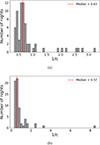 |
Fig. 1. Distributions of the 1/η metric for the polarization degree (Π; panel a) and the polarization angle (Ψ; panel b), across all 65 observing nights. The vertical dashed red line in each panel indicates the median of the distribution, which also serves as the threshold separating variable from non-variable nights. |
Given the stochastic nature of blazar variability, we complemented the 1/η criterion by computing for each night both the standard deviation of the measurements and their median uncertainty. If a night exceeds the 1/η threshold, we assessed whether the amplitude of its variation is significant by comparing the standard deviation with the median uncertainty within the night. If the standard deviation is larger than the median uncertainty, the observed excursions are likely intrinsic to the source and not due to the signal-to-noise of the observations. Using this additional check, we were able to evaluate the overall behavior of the fluctuations–independent of temporal structure–and remain robust against outliers. By combining the 1/η metric, which is sensitive to temporal correlations, with the standard deviation relative to the measurement uncertainties, which reflects the amplitude of variations, we obtained an overall more robust criterion for identifying genuine variability.
In Fig. 2 we present the results for BL Lacertae (J2202+4216), which serves as an example of a source exhibiting clear intra-night variability. In contrast, Fig. 3 shows the results for J1542+6129, a case with no significant intra-night variability. Figure 4 illustrates a source whose polarization degree (Π) remains very close to zero, resulting in many non-detections (Π < 3 ⋅ δΠ) throughout the night. For this target, we binned the data in pairs (combining two consecutive images) and retained only the detection points. It is important to note that this binning procedure was performed on the Stokes Q and Stokes U space, and then the Π and Ψ were recomputed according to the following standard equations,
 (2)
(2)
 (3)
(3)
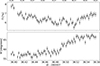 |
Fig. 2. Intra-night RoboPol observations of BL Lac (example of a source showing polarization variability). Top: Polarization degree. Bottom: Polarization angle. The observations have an average cadence of 3.31 minutes. |
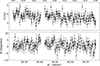 |
Fig. 3. Intra-night RoboPol observations of J1542+6129 (example of a source without polarization variability). Top: Polarization degree. Bottom: Polarization angle. The observations have an average cadence of 2.29 minutes. |
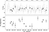 |
Fig. 4. Intra-night RoboPol observations of J2148+0657 (example of a source with binned observations; two consecutive images combined). The gray points show the unbinned observations. Top: Polarization degree. Bottom: Polarization angle. The upper limits have been omitted for clarity. The observations have an average cadence of 12.99 minutes. |
3. Results
Of the 65 observing nights, 37 show evidence of variability in either the polarization degree or angle. Table 1 presents our results for all sources, with columns indicating the total number of observations for each source and the number of nights we find evidence of polarization variability. The reported values of Π and Ψ correspond to the median (and standard deviation) over all available measurements (averaged in Stokes Q-U space), rather than intra-night values, which are available in the Harvard dataverse repository. Overall, we find a median Π of ≈5% with a minimum of ≈1% and a maximum of ≈14%, consistent with previous RoboPol observations (Angelakis et al. 2016). Intra-night variable blazars exhibit a variety of variability patterns, from smooth continuous changes throughout a single night (e.g., Fig. 2) to more abrupt stochastic variations.
Given that our sample is statistically well defined and the monitoring was performed blindly (i.e., without selecting particular nights), 56.9% (37 out of 65 nights) of all blazar observations should show intra-night variability of the polarization parameters in a magnitude-limited sample. Out of the twenty sources in our sample, only four did not show variability in either Π or Ψ. However, three out of the four sources show low Π, < 5%, which could have prevented us from uncovering variability patterns due to signal-to-noise limitations. Nevertheless, that would suggest that 80% of LSP blazars in a blind survey show intra-night variability. Moreover, seven sources (35% of the sample) show variability on every observing night, while the overall duty cycle is 61.9% (average Nvar/N from all the sources in the sample–see Table 1). The amplitude of the variations is typically ΔΠ < 5% and ΔΨ < 20°. We do not find strong evidence of a preference of variability in Π or Ψ.
To compare our results with archival data, we used measurements from the long-term monitoring survey conducted at the Skinakas Observatory from 2013 to 2017 (Blinov et al. 2021). We calculated the median and standard deviation of the Stokes parameters for each source, which we then converted to Π and Ψ. Figure 5 presents this comparison for both Π and Ψ. Our intra-night results are shown along the x-axes, and the archival values are plotted on the y-axes. We find an overall good agreement between datasets despite them having completely different times and timescales. Intra-night Π shows the largest departures from the long-term behavior, with sources becoming both more and less polarized. On the other hand, the intra-night Ψ shows an almost perfect agreement with the long-term observations.
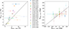 |
Fig. 5. Comparison of our results (intra-night monitoring) with those of the previous survey (long-term monitoring; Blinov et al. 2021). Left: Polarization degree (Π). Right: Polarization angle (Ψ). Different colors indicate different sources. The dashed black line in each panel marks equality (y = x) and illustrates the agreement between the long-term and intra-night monitoring observations. |
4. Conclusions
We have presented a pilot study of 20 blazars selected from the RoboPol sample with strict statistical criteria. The sources were observed over a total of 65 nights in 2024 and early 2025. Our dataset is supplemented by observations from Calar Alto, Perkins, and the Sierra Nevada monitoring programs. We find that the majority of our observations show intra-night variability in either Π or Ψ, with no strong evidence of a preference in either Π or Ψ. Only four sources did not show variability; however, the observations for three out of the four were taken in low Π states. Future observations of these sources have the potential to reveal variability if taken in higher polarization states. For the other sources, the duty cycle for detecting intra-night variability in a blind survey has a median of 61.9%, while the amplitude of the observed variability is small, with changes of typically no more than 5% in the polarization degree and 20 degrees in the polarization angle.
Comparing our campaign with the long-term observations taken by RoboPol between 2013 and 2017 (Blinov et al. 2021), we find that the polarization degree has changed in a number of sources, showing both lower and higher polarization. Interestingly, the intra-night polarization angle appears to be consistent with the long-term behavior. Models of magnetic field variability in blazars usually invoke shocks moving inside the jet (e.g., Marscher & Gear 1985; Marscher et al. 2008, 2010; Liodakis et al. 2020), magnetic reconnection (e.g., Hosking & Sironi 2020; Zhang et al. 2020), kink instabilities (e.g., Dong et al. 2020; Jorstad et al. 2022), or turbulence (e.g., Marscher 2014; Peirson & Romani 2018). The long-term stability of the polarization angle indicates the presence of a persistent magnetic field orientation. This could be due to either the presence of a recollimation shock or the presence of a large-scale helical magnetic field permeating the jet (e.g., Clausen-Brown et al. 2011; Hovatta et al. 2012; Paraschos et al. 2024). On the other hand, the minute-timescale low-amplitude variability, as well as the much lower observed polarization degree compared to the theoretical maximum for synchrotron radiation (∼70%), indicates the presence of a significant turbulent magnetic field component. Therefore, models that can accommodate both ordered and disordered magnetic field components (e.g., Marscher 2014) are necessary to account for the observed phenomenology.
Since early 2025 we have been performing additional high-cadence intra-night observations of blazars with the highest variability duty cycle using RoboPol, aiming to detect the predicted intra-night polarization angle rotations. These observations will be discussed in an upcoming publication.
Acknowledgments
We thank the anonymous referee for useful comments that helped improve the paper. The study was funded by the European Union ERC-2022-STG–BOOTES–101076343. Views and opinions expressed are however those of the author(s) only and do not necessarily reflect those of the European Union or the European Research Council Executive Agency. Neither the European Union nor the granting authority can be held responsible for them. The Perkins Telescope Observatory, located in Flagstaff, AZ, USA, is owned and operated by Boston University. Observations at the Perkins telescope were supported by NASA Fermi Guest Investigator grant 80NSSC23K1507. Some of the data are based on observations collected at the Centro Astronómico Hispano en Andalucía (CAHA), operated jointly by Junta de Andalucía and Consejo Superior de Investigaciones Científicas (IAA-CSIC). Some of the data are based on observations collected at the Observatorio de Sierra Nevada; which is owned and operated by the Instituto de Astrofísica de Andalucía (IAA-CSIC). The IAA-CSIC co-authors acknowledge financial support from the Spanish “Ministerio de Ciencia e Innovación” (MCIN/AEI/ 10.13039/501100011033) through the Center of Excellence Severo Ochoa award for the Instituto de Astrofíisica de Andalucía-CSIC (CEX2021-001131-S), and through grants PID2019-107847RB-C44 and PID2022-139117NB-C44. D.B. acknowledges support from the European Research Council (ERC) under the Horizon ERC Grants 2021 programme under grant agreement No. 101040021.
References
- Agarwal, A., Mihov, B., Agrawal, V., et al. 2023, ApJS, 265, 51 [Google Scholar]
- Agudo, I., Molina, S. N., Gómez, J. L., et al. 2012, Int. J. Mod. Phys. Conf. Ser., 8, 299 [NASA ADS] [CrossRef] [Google Scholar]
- Agudo, I., Liodakis, I., Otero-Santos, J., et al. 2025, ApJ, 985, L15 [Google Scholar]
- Ajello, M., Angioni, R., Axelsson, M., et al. 2020, ApJ, 892, 105 [NASA ADS] [CrossRef] [Google Scholar]
- Angelakis, E., Hovatta, T., Blinov, D., et al. 2016, MNRAS, 463, 3365 [NASA ADS] [CrossRef] [Google Scholar]
- Bachev, R., Semkov, E., Strigachev, A., et al. 2012, MNRAS, 424, 2625 [CrossRef] [Google Scholar]
- Bachev, R., Tripathi, T., Gupta, A. C., et al. 2023, MNRAS, 522, 3018 [NASA ADS] [CrossRef] [Google Scholar]
- Blandford, R., Meier, D., & Readhead, A. 2019, ARA&A, 57, 467 [NASA ADS] [CrossRef] [Google Scholar]
- Blinov, D., Pavlidou, V., Papadakis, I., et al. 2015, MNRAS, 453, 1669 [NASA ADS] [CrossRef] [Google Scholar]
- Blinov, D., Pavlidou, V., Papadakis, I. E., et al. 2016a, MNRAS, 457, 2252 [NASA ADS] [CrossRef] [Google Scholar]
- Blinov, D., Pavlidou, V., Papadakis, I., et al. 2016b, MNRAS, 462, 1775 [Google Scholar]
- Blinov, D., Pavlidou, V., Papadakis, I., et al. 2018, MNRAS, 474, 1296 [CrossRef] [Google Scholar]
- Blinov, D., Kiehlmann, S., Pavlidou, V., et al. 2021, MNRAS, 501, 3715 [NASA ADS] [CrossRef] [Google Scholar]
- Blinov, D., Maharana, S., Bouzelou, F., et al. 2023, A&A, 677, A144 [NASA ADS] [CrossRef] [EDP Sciences] [Google Scholar]
- Capecchiacci, S., Liodakis, I., Middei, R., et al. 2025, A&A, 703, A19 [NASA ADS] [CrossRef] [EDP Sciences] [Google Scholar]
- Chen, C.-T. J., Liodakis, I., Middei, R., et al. 2024, ApJ, 974, 50 [NASA ADS] [CrossRef] [Google Scholar]
- Clausen-Brown, E., Lyutikov, M., & Kharb, P. 2011, MNRAS, 415, 2081 [Google Scholar]
- Di Gesu, L., Donnarumma, I., Tavecchio, F., et al. 2022, ApJ, 938, L7 [CrossRef] [Google Scholar]
- Di Gesu, L., Marshall, H. L., Ehlert, S. R., et al. 2023, Nat. Astron., 7, 1245 [NASA ADS] [CrossRef] [Google Scholar]
- Dong, L., Zhang, H., & Giannios, D. 2020, MNRAS, 494, 1817 [NASA ADS] [CrossRef] [Google Scholar]
- Escudero Pedrosa, J., Morcuende Parrilla, D., & Otero-Santos, J. 2024a, IOP4 [Google Scholar]
- Escudero Pedrosa, J., Agudo, I., Morcuende, D., et al. 2024b, AJ, 168, 84 [Google Scholar]
- Fraija, N., Benítez, E., Hiriart, D., et al. 2017, ApJS, 232, 7 [Google Scholar]
- Goyal, A., Gopal-Krishna, Wiita, P. J., et al. 2012, A&A, 544, A37 [NASA ADS] [CrossRef] [EDP Sciences] [Google Scholar]
- Hosking, D. N., & Sironi, L. 2020, ApJ, 900, L23 [NASA ADS] [CrossRef] [Google Scholar]
- Hovatta, T., & Lindfors, E. 2019, New Astron. Rev., 87, 101541 [CrossRef] [Google Scholar]
- Hovatta, T., Lister, M. L., Aller, M. F., et al. 2012, AJ, 144, 105 [Google Scholar]
- Jorstad, S. G., Marscher, A. P., Raiteri, C. M., et al. 2022, Nature, 609, 265 [NASA ADS] [CrossRef] [Google Scholar]
- Kiehlmann, S., Blinov, D., Liodakis, I., et al. 2021, MNRAS, 507, 225 [NASA ADS] [CrossRef] [Google Scholar]
- King, O. G., Blinov, D., Ramaprakash, A. N., et al. 2014, MNRAS, 442, 1706 [NASA ADS] [CrossRef] [Google Scholar]
- Kouch, P. M., Liodakis, I., Middei, R., et al. 2024, A&A, 689, A119 [NASA ADS] [CrossRef] [EDP Sciences] [Google Scholar]
- Liodakis, I., Blinov, D., Jorstad, S. G., et al. 2020, ApJ, 902, 61 [NASA ADS] [CrossRef] [Google Scholar]
- Liodakis, I., Marscher, A. P., Agudo, I., et al. 2022, Nature, 611, 677 [CrossRef] [Google Scholar]
- Liodakis, I., Kiehlmann, S., Marscher, A. P., et al. 2024, A&A, 689, A200 [NASA ADS] [CrossRef] [EDP Sciences] [Google Scholar]
- Liodakis, I., Zhang, H., Boula, S., et al. 2025, A&A, 698, L19 [NASA ADS] [CrossRef] [EDP Sciences] [Google Scholar]
- Marscher, A. P. 2014, ApJ, 780, 87 [Google Scholar]
- Marscher, A. P., & Gear, W. K. 1985, ApJ, 298, 114 [Google Scholar]
- Marscher, A. P., & Jorstad, S. G. 2021, Galaxies, 9, 27 [NASA ADS] [CrossRef] [Google Scholar]
- Marscher, A. P., Jorstad, S. G., D’Arcangelo, F. D., et al. 2008, Nature, 452, 966 [Google Scholar]
- Marscher, A. P., Jorstad, S. G., Larionov, V. M., et al. 2010, ApJ, 710, L126 [Google Scholar]
- Marscher, A. P., Di Gesu, L., Jorstad, S. G., et al. 2024, Galaxies, 12, 50 [NASA ADS] [CrossRef] [Google Scholar]
- Marshall, H. L., Liodakis, I., Marscher, A. P., et al. 2024, ApJ, 972, 74 [NASA ADS] [CrossRef] [Google Scholar]
- McCall, C., Jermak, H. E., Steele, I. A., et al. 2024, MNRAS, 528, 4702 [NASA ADS] [CrossRef] [Google Scholar]
- Middei, R., Liodakis, I., Perri, M., et al. 2023, ApJ, 942, L10 [NASA ADS] [CrossRef] [Google Scholar]
- Negi, V., Gopal-Krishna, Joshi, R., et al. 2023, MNRAS, 522, 5588 [Google Scholar]
- Otero-Santos, J., Piirola, V., Escudero Pedrosa, J., et al. 2024, AJ, 167, 137 [Google Scholar]
- Panopoulou, G., Tassis, K., Blinov, D., et al. 2015, MNRAS, 452, 715 [Google Scholar]
- Paraschos, G. F., Debbrecht, L. C., Kramer, J. A., et al. 2024, A&A, 686, L5 [NASA ADS] [CrossRef] [EDP Sciences] [Google Scholar]
- Pavlidou, V., Angelakis, E., Myserlis, I., et al. 2014, MNRAS, 442, 1693 [NASA ADS] [CrossRef] [Google Scholar]
- Peirson, A. L., & Romani, R. W. 2018, ApJ, 864, 140 [NASA ADS] [CrossRef] [Google Scholar]
- Peirson, A. L., Negro, M., Liodakis, I., et al. 2023, ApJ, 948, L25 [NASA ADS] [CrossRef] [Google Scholar]
- Sagar, R., Stalin, C. S., Gopal-Krishna, & Wiita, P. J. 2004, MNRAS, 348, 176 [NASA ADS] [CrossRef] [Google Scholar]
- Sokolovsky, K. V., Gavras, P., Karampelas, A., et al. 2017, MNRAS, 464, 274 [CrossRef] [Google Scholar]
- Villforth, C., Nilsson, K., Østensen, R., et al. 2009, MNRAS, 397, 1893 [CrossRef] [Google Scholar]
- Zhang, H., Li, X., Giannios, D., et al. 2020, ApJ, 901, 149 [CrossRef] [Google Scholar]
All Tables
All Figures
|
Fig. 1. Distributions of the 1/η metric for the polarization degree (Π; panel a) and the polarization angle (Ψ; panel b), across all 65 observing nights. The vertical dashed red line in each panel indicates the median of the distribution, which also serves as the threshold separating variable from non-variable nights. |
| In the text | |
|
Fig. 2. Intra-night RoboPol observations of BL Lac (example of a source showing polarization variability). Top: Polarization degree. Bottom: Polarization angle. The observations have an average cadence of 3.31 minutes. |
| In the text | |
|
Fig. 3. Intra-night RoboPol observations of J1542+6129 (example of a source without polarization variability). Top: Polarization degree. Bottom: Polarization angle. The observations have an average cadence of 2.29 minutes. |
| In the text | |
|
Fig. 4. Intra-night RoboPol observations of J2148+0657 (example of a source with binned observations; two consecutive images combined). The gray points show the unbinned observations. Top: Polarization degree. Bottom: Polarization angle. The upper limits have been omitted for clarity. The observations have an average cadence of 12.99 minutes. |
| In the text | |
|
Fig. 5. Comparison of our results (intra-night monitoring) with those of the previous survey (long-term monitoring; Blinov et al. 2021). Left: Polarization degree (Π). Right: Polarization angle (Ψ). Different colors indicate different sources. The dashed black line in each panel marks equality (y = x) and illustrates the agreement between the long-term and intra-night monitoring observations. |
| In the text | |
Current usage metrics show cumulative count of Article Views (full-text article views including HTML views, PDF and ePub downloads, according to the available data) and Abstracts Views on Vision4Press platform.
Data correspond to usage on the plateform after 2015. The current usage metrics is available 48-96 hours after online publication and is updated daily on week days.
Initial download of the metrics may take a while.