| Issue |
A&A
Volume 704, December 2025
|
|
|---|---|---|
| Article Number | L14 | |
| Number of page(s) | 5 | |
| Section | Letters to the Editor | |
| DOI | https://doi.org/10.1051/0004-6361/202557622 | |
| Published online | 12 December 2025 | |
Letter to the Editor
The dispersion in pulsar γ-ray efficiency
1
Institute of Space Sciences (ICE, CSIC), Campus UAB, Carrer de Can Magrans s/n, 08193 Barcelona, Spain
2
Institut d’Estudis Espacials de Catalunya (IEEC), 08034 Barcelona, Spain
3
Institució Catalana de Recerca i Estudis Avançats (ICREA), E-08010 Barcelona, Spain
★ Corresponding author: This email address is being protected from spambots. You need JavaScript enabled to view it.
Received:
9
October
2025
Accepted:
26
November
2025
Abstract
Context. The observational efficiency of pulsars, defined as the ratio of the observationally derived isotropic-equivalent luminosity, 4πdobs2Fobs, where Fobs is the average pulsed energy flux of a pulsar and dobs is its estimated distance, to its energy budget, shows a wide range of values. This dispersion is believed to be a combination of beaming effects, different geometries, and case-by-case variability of the emission mechanism efficiency, but it is not clear in what proportion.
Aims. In this work we focused on the γ-ray range and analysed the four main ingredients that likely contribute to this dispersion: the geometrical term arising from the anisotropic emission (beaming), viewing and inclination angles, the uncertainty on the pulsar distance, the uncertainty on the moment of inertia, and the intrinsic efficiency of the mechanism producing the γ-ray emission.
Methods. Estimating the expected ranges of the moment of inertia and the distance errors, and considering a geometrical and spectral model that we have recently used to fit the light curves and spectra of the entire γ-ray pulsar population, we estimate the a priori distribution of the first three ingredients in order to obtain the a posteriori distribution of the intrinsic efficiency of the mechanism.
Results. We found the latter to peak at ∼5 − 15% (depending on the trial distribution) and to have a dispersion of around one order of magnitude. That is, we found the intrinsic efficiency of the mechanism to be the leading factor in the observed dispersion. In addition, we found little sensitivity of these results on different distributions of the estimated pulsar distance errors, and saw that the weak, alleged correlation with the spin-down power can only explain part of the observed dispersion. This methodology can be easily applied to other geometrical models of the emission, to test the sensitivity of these results on the beaming distribution.
Key words: pulsars: general / gamma rays: stars
© The Authors 2025
 Open Access article, published by EDP Sciences, under the terms of the Creative Commons Attribution License (https://creativecommons.org/licenses/by/4.0), which permits unrestricted use, distribution, and reproduction in any medium, provided the original work is properly cited.
This article is published in open access under the Subscribe to Open model. This email address is being protected from spambots. You need JavaScript enabled to view it. to support open access publication.
1. Introduction
The observational efficiency ηobs is defined as the ratio of the derived isotropic-equivalent luminosity of the pulsar to the pulsar spin-down power:
 (1)
(1)
where Fobs is the average pulsed energy flux of a pulsar, dobs is the estimated distance, I0 = 1045 g/cm2 is the conventional value of the moment of inertia, and Ω and ̇Ω are the observed spin frequency and its time derivative, respectively. In this work we focus on the γ-ray range of Fermi-LAT (100 MeV – 300 GeV), for which the values of ηobs from the Third Fermi Pulsar Catalog (Smith et al. 2023, hereafter 3PC) show a wide dispersion, with values ranging from ∼0.02% up to ∼200%. The uncertainty on the pulsar distances and the assumed fixed value of the beaming factor fΩ = 1, are usually mentioned as the origin of this dispersion. Here we consider these two factors, plus the uncertainty on the moment of inertia (neglecting the uncertainties on the timing parameters since they are measured with notable precision), to factorize the combined efficiency as
 (2)
(2)
hereafter conveniently considered in its logarithmic version:
 (3)
(3)
We label with an asterisk two quantities (the real distance d* and moment of inertia of the star I*) which are unknown and might differ from the estimated values, so that ϵd := dobs2/d*2 and ϵI := I*/I0 encode the uncertainties on the distance and moment of inertia, respectively. The factor  is the intrinsic efficiency of the mechanism converting the rotational energy losses into γ-ray emission (via particle acceleration), with ⟨F⟩ being the average γ-ray flux emitted over the sky, i.e. the entire magnetospheric emission in γ-rays. The beaming factor fΩ := ⟨F⟩/Fobs, defined as in e.g. Watters et al. (2009), is the ratio of the total pulsed emission of the pulsar averaged over the sky ⟨F⟩ to the phase-averaged emission detected by a given observer Fobs. This depends on the strongly anisotropic (beamed) emission of the pulsar, the magnetospheric configuration (in particular, the inclination angle ψΩ between the rotational axis and the magnetic moment), and the viewing angle θobs between the pulsar equatorial plane and the line of sight of the observer. Therefore, the beaming factor can be estimated using a geometrical model of the magnetospheric emission. If the flux intercepted by the observer is exactly the averaged flux over the sky, fΩ = 1. Observers in a line of sight that crosses the bulk of the emission have small values fΩ < 1, while those observers that intercept the directions with a lower-than-average flux have fΩ > 1. Lucky observers with small beaming factors will estimate a higher observational efficiency than the average observers, which explains the possibility of measuring ηobs ≳ 100%.
In this study we quantified the a priori distribution of values of three terms (fΩ, ϵd, and ϵI), in order to obtain an a posteriori distribution of the physical mechanism efficiency ηrad, by comparison with the observed distribution of ηobs. We used the standard deviation as a measure of the dispersion of a distribution.
2. Ingredients contributing to the dispersion of the observational γ-ray efficiency
2.1. Beaming factor, fΩ
The beaming factor, fΩ, is here quantitatively estimated using our spectral-geometrical models (for details, see Viganò et al. 2015; Viganò & Torres 2019; Íñiguez-Pascual et al. 2024, 2025 and references therein). These models were built with an effective approach, have a minimal set of parameters, and are based on following the dynamics of charged magnetospheric particles accelerated by an electric field. The dynamics were computed consistently with the associated synchro-curvature emission. Defining an emitting region that mimics the current sheet shape seen in force-free electrodynamics (FFE) and particle-in-cell (PIC) simulations, we computed the emission maps on the sky, and the light curves for any observer. Synthetic spectra and light curves were fitted to the observed 3PC sample (Íñiguez-Pascual et al. 2024, 2025).
For a given choice of the free spectral parameters and inclination angle ψΩ, the synthetic sky maps consist of a discrete set of fluxes F(θobs, i, ϕj; ΨΩ), where ϕj ∈ [0, 2π) indicates the rotational phase of the pulsar, and θobs, i ∈ (0, π) the observer. For this work we used Ni = 51 observers and a number of phase bins, Nj, as defined in Íñiguez-Pascual et al. (2025), typically 100. We do not discuss here the energy dependence of sky maps and light curves (see Íñiguez-Pascual et al. 2025): fluxes are integrated over the Fermi-LAT energy range. The average flux over the sky, ⟨F⟩, and the phase-averaged flux detected by the observer, θi, Fobs, i, are
 (4)
(4)
 (5)
(5)
and their ratio gives the synthetic beaming factor for each observer, for every sky map. To obtain the fΩ distribution, we considered the 226 3PC pulsars we fitted in Íñiguez-Pascual et al. (2025). For each of them, we generated 30 emission maps, changing ψΩ, uniformly distributed between 3° to 90°. For a given sky map, we discarded the observers detecting no flux or a flux below a threshold of 5% of the maximum of the map, which are about 40% of the total (Íñiguez-Pascual et al. 2025). Therefore, for every pulsar, we were left with about ∼103 synthetic light curves, each one having a value of fΩ. Importantly, the fΩ distributions obtained from different pulsars are all very similar despite the different spectral and timing (Ω,  ) configurations among the pulsars considered (which implies different free parameters of our spectral model; see Íñiguez-Pascual et al. 2025). This is due to what we found in Íñiguez-Pascual et al. (2024): the geometry (ψΩ and θobs) plays a dominant role in defining the emission maps in γ-rays, thus effectively decoupling the sky maps (and the fΩ distributions) from the observed timing and spectral properties. Therefore, the impact of the geometrical configuration of the pulsar and its emission region on fΩ overshadows that of the timing and spectral parameters: the fΩ distribution as independent of them.
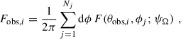
The top left panel of Fig. 1 shows the histogram of the distribution of the logarithm of fΩ. Not surprisingly, it peaks around fΩ ∼ 1, has a standard deviation of 0.29 and is asymmetric, with a more pronounced tail at small values rather than large ones (not only due to the logarithmic representation). Although our results might depend on the assumed region emission shape, our fΩ distribution looks qualitatively similar to results obtained in other theoretical studies considering either gap models (Pierbattista et al. 2012) or complex numerical simulations (Kalapotharakos et al. 2023; Cerutti et al. 2025).
 |
Fig. 1. Probability density of the terms forming log10ηobs. Top: log10fΩ (left) and log10ϵI (right). Bottom: log10ϵd from different prescriptions, P(Δ) = 𝒩 (left) and P(ϵd) = 𝒩 (right). |
2.2. Uncertainty on the moment of inertia, ϵI
A conventional value of I0 = 1045 g/cm2 is usually assumed when computing the rotational energy losses. However, each pulsar has its own I* since it depends on the mass and radius, although these are generally unknown. In addition, the equation of state (EoS) for cold dense matter is still not known precisely, which is reflected in the uncertainty on the neutron star (NS) characteristic mass-radius (M(R)) relation.
To take into account both effects, we can estimate I* using the expression presented by Bejger & Haensel (2002), which, considering a large sample of NS structures built with many different available EoSs and masses, found a best-fitting effective expression for the moment of inertia: I = a(x)MR2, with x = (M/M⊙)(km/R) and a(x) = x/(0.1 + 2x) for x ≤ 0.1 and  for x > 0.1. In order to obtain an informed a priori distribution of values of I*, we also need the distribution of M and R of NSs. Masses can be estimated in several cases, mainly when in binary systems (Özel & Freire 2016), and their values are well described by a skew normal distribution, 𝒮𝒩 (Kiziltan et al. 2013), whose parameters are the mean μ, the standard deviation σ, and the skewness α. Using the best-fitting parameters to the most updated available sample1, we then assume an a priori distribution of the masses (in solar masses) P(M[M⊙]) = 𝒮𝒩(μ = 1.20, σ = 0.31, α = 14.03). Given the substantial lack of precise constraints on the radius, we take R to be distributed as a Gaussian P(R[km]) = 𝒩(μ = 12.0, σ = 1.0), a representative distribution, where the dispersion assumed here is compatible with the relatively vertical shape of the M(R) curve for most EoSs. Given the lesser role played by the moment of inertia (see below), we do not explore other mean values of R.
Sampling (∼103) values of R and M from the mentioned distributions with an acceptance-rejection method, we can obtain a distribution of physically motivated values of the moment of inertia. Dividing it by I0 gives the uncertainty term associated with the moment of inertia ϵI. The right top panel of Fig. 1 shows the histogram of the distribution of its logarithm. It is centred at log10ϵI ∼ 0.2 and has a standard deviation of 0.09, smaller than that of the distributions log10fΩ and log10ϵd (see below).
2.3. Uncertainty on the distance, ϵd
The real distance to a pulsar from Earth, d*, is unknown. The observationally estimated values, dobs, normally have large uncertainties and are obtained with different methods, for example the dispersion measurement method, parallax, or kinetic method. As a proxy of the distance uncertainties distribution, we take the average of the relative distance errors of the pulsar sample, as quoted in the 3PC, which is σd, rel = 0.341. In the absence of a better estimation for the error distribution, we consider two cases. In the first case, we assume that the relative error Δ := (d* − dobs)/dobs follows a Gaussian distribution, with μ = 0 and σ = σd, rel. We then sample (∼106) Δ values with an inverse transform method, and obtain the corresponding set of values ϵd = (Δ + 1)−2. The second choice is to instead consider the distribution of ϵd itself as a Gaussian (sampling ∼106 values), with μ = 1 and σϵ, d = (σd, rel + 1)−2 = 0.556. The resulting P(log10ϵd) for the two choices (left panels of Fig. 2) differ in shape, but only slightly in standard deviation (0.38 and 0.31, respectively).
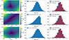 |
Fig. 2. Results of the fitting to find the distribution of ηrad. The top (middle) row shows those obtained using the distance uncertainty distributed as P(Δ) = 𝒩, with a Gaussian (skew normal) as the trial distribution. The bottom row were obtained with the distance uncertainty distributed as P(ϵd) = 𝒩, with a Gaussian as the trial distribution. From left to right: contour plot of DKS in the space of parameters μrad − σrad (in the skew normal case we collapsed all the contours for the different α considered taking the smallest DKS for each pair μrad − σrad), best-fitting distribution of log10ηrad, overlapped distribution of log10ηobs (red), and joint distribution (blue). |
3. Distribution of the mechanism efficiency
The rotational energy losses represent the budget powering pulsar high-energy emission. However, which fraction is ultimately converted into emitted radiation is not known exactly since it depends on the details of every step of the conversion: Poynting flux → particle creation and acceleration → synchro-curvature radiation (in γ-ray range).
We assumed a trial distribution for log10ηrad and, assuming that the four distributions on the right-hand side of Eq. (3) are independent of each other, their sum (hereafter referred to as joint distribution) is simply obtained by performing a Monte Carlo sampling of each distribution and summing the values (see e.g. Chapter 3 of Springer 1979). We then compared it with the distribution of the logarithm of the observational efficiency log10ηobs by applying a Kolmogorov–Smirnov (KS) test. The metric of the KS test, DKS, measures the similarity between two distributions, by using their empirical distribution functions. We minimized DKS by scanning the space of parameters of the trial distribution and picking up the set of parameters giving a smaller DKS. The best-fitting set of parameters defining the distribution of log10ηrad is the one that generates a joint distribution most closely resembling log10ηobs. Finally, we obtained the dispersion and peak position of the best-fitting trial distribution.
Table 1 compares the best-fitting parameters of the trial distributions (Gaussian or skew normal) of log10ηrad for the two different prescriptions of distance uncertainties. The resulting joint distributions are shown in the right column of Fig. 2, compared with log10ηobs. In all cases, the dispersion of log10ηrad is similar, with standard deviations of 0.42 − 0.56, which corresponds to around one order of magnitude in ηrad, regardless of the different shapes of distributions. The best-fitting a posteriori distributions peak at a value  , which changes between ∼5 and ∼15%; the change is mainly due to the different shapes of the trial distributions.
Best-fitting parameters of the trial distributions of P(log10ηrad) for different distributions of distance uncertainty.
Note that in all cases there is a slight mismatch at low ηobs values. This can be produced by the observational biases that affect this region: the small values may be a result of a low flux close to the Fermi-LAT sensitivity. Thus, the comparison at low values is not informative and we do not focus on them. Instead, note that the cases with P(Δ) = 𝒩 have a tail at high values (log10ηrad > 10), which are incompatible with the observed distribution regardless of the shape of the distribution P(log10ηrad), and is due to cases with very large log10ϵd ≳ 1 (i.e. an order of magnitude overestimation of d*2). Such a tail is indeed much less visible if we consider the distance uncertainty distributed as P(ϵd) = 𝒩(1, σϵ, d) because the latter has fewer extremely high values. Moreover, for the latter case, we explored the sensitivity of the fitting on the dispersion of the a priori distribution P(ϵd) by taking σϵ, d = 0.2 and 0.7 instead of 0.556. The result is that the peak position of the mechanism efficiency distribution barely changes, while its standard deviation change by only ∼30% between the two extremes of σϵ, d.
Overall, this indicates a minor influence of the ϵd prescription on the best-fitting a posteriori distribution of ηrad. It also implies that ηrad is the term dominating the dispersion of ηobs.
4. Discussion
The dispersion of the observational γ-ray efficiency ηobs can be explained with the four ingredients we have introduced here: fΩ, ϵd, ϵI, and ηrad. We found ηrad to be a main contributor, at least as relevant as the distance errors and the fΩ distribution coming from our geometrical model. The contribution of ϵI is smaller compared to the other three terms, which indicates that assuming I = 1045g/cm2 for all pulsars does not significantly affect the observational efficiency values. With the two trial distributions we considered for the efficiency of the physical mechanism of γ-ray emission ηrad, we found a peak position of around 5 − 15%, with a dispersion of approximately one order of magnitude. The same conclusion was obtained for a few different trial distributions of ηrad and/or prescriptions regarding the uncertainty on the pulsar distances.
The average values we found agree with the results found in complex magnetospheric simulations (FFE or PIC), in which ∼10 − 20% of the Poynting flux is dissipated in the first 1 − 2 light cylinder radius of the equatorial current sheet (Carrasco et al. 2018; Cerutti et al. 2020; Hakobyan et al. 2023). The dissipated Poynting flux in the current sheet is converted into acceleration of particles, which then emit the high-energy radiation we detect. In our spectral-geometrical models, the γ-ray emission typically represents ≳95% of the total synchro-curvature radiation, in agreement with the tiny (always less than 1%) X-ray observational efficiencies of Fermi pulsars reported in e.g. Marelli et al. (2011). The mean values of ηrad also agree with the fact that pulsar wind nebulae, which are powered by the pulsar itself, require a significant amount of its energy.
The relatively large dispersion of the inferred ηrad distribution could be due to different factors. The alleged weak correlation 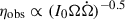 reported in the 3PC can explain a part of the dispersion (see Appendix A). Other sources of dispersion could be differences in e.g. magnetic field topology at the surface or beyond the light cylinder (boundary conditions with the surrounding medium). General relativity effects on the torque and pair production, which depend on the compactness (Ruiz et al. 2014; Philippov et al. 2015; Carrasco et al. 2018), could also be a minor ingredient for dispersion. Note that the precise shape of the distribution of ηrad remains unconstrained with our methodology since a good fit is obtained with the two trial distributions. In this regard, note that the tail with very high arguably unphysical values ≳50% of efficiency is actually not needed: imposing a skew normal distribution, or, similarly, a cutoff at ηrad ≳ 30%, essentially provide the same results in terms of inferred mean and dispersion.
Finally, this simple methodology can be implemented to test whether different geometrical models, with their own fΩ distributions, can change the results here presented.
Acknowledgments
We thank the referee David Smith for his valuable comments. This work has been supported by PID2024-155316NB-I00 funded by MCIN/AEI/10.13039/501100011033, CSIC PIE 202350E189, the Spanish program Unidad de Excelencia María de Maeztu CEX2020-001058-M and by European Union NextGeneration EU (PRTR-C17.I1). DIP has been supported by the FPI pre-doctoral fellowship PRE2021-100290 from the Spanish MCIU and his work has been carried out within the framework of the doctoral programme in Physics of the UAB. DV is funded by the European Research Council Starting Grant IMAGINE, No. 948582.
References
- Bejger, M., & Haensel, P. 2002, A&A, 396, 917 [NASA ADS] [CrossRef] [EDP Sciences] [Google Scholar]
- Carrasco, F., Palenzuela, C., & Reula, O. 2018, Phys. Rev. D, 98, 023010 [Google Scholar]
- Cerutti, B., Philippov, A. A., & Dubus, G. 2020, A&A, 642, A204 [NASA ADS] [CrossRef] [EDP Sciences] [Google Scholar]
- Cerutti, B., Figueiredo, E., & Dubus, G. 2025, A&A, 695, A93 [NASA ADS] [CrossRef] [EDP Sciences] [Google Scholar]
- Hakobyan, H., Philippov, A., & Spitkovsky, A. 2023, ApJ, 943, 105 [NASA ADS] [CrossRef] [Google Scholar]
- Íñiguez-Pascual, D., Torres, D. F., & Viganò, D. 2024, MNRAS, 530, 1550 [CrossRef] [Google Scholar]
- Íñiguez-Pascual, D., Torres, D. F., & Viganò, D. 2025, MNRAS, 541, 806 [Google Scholar]
- Kalapotharakos, C., Wadiasingh, Z., Harding, A. K., & Kazanas, D. 2023, ApJ, 954, 204 [NASA ADS] [CrossRef] [Google Scholar]
- Kiziltan, B., Kottas, A., De Yoreo, M., & Thorsett, S. E. 2013, ApJ, 778, 66 [NASA ADS] [CrossRef] [Google Scholar]
- Marelli, M., De Luca, A., & Caraveo, P. A. 2011, ApJ, 733, 82 [Google Scholar]
- Özel, F., & Freire, P. 2016, ARA&A, 54, 401 [Google Scholar]
- Philippov, A. A., Cerutti, B., Tchekhovskoy, A., et al. 2015, ApJ, 815, L19 [NASA ADS] [CrossRef] [Google Scholar]
- Pierbattista, M., Grenier, I. A., Harding, A. K., & Gonthier, P. L. 2012, A&A, 545, A42 [NASA ADS] [CrossRef] [EDP Sciences] [Google Scholar]
- Ruiz, M., Paschalidis, V., & Shapiro, S. L. 2014, Phys. Rev. D, 89, 084045 [Google Scholar]
- Smith, D. A., Abdollahi, S., Ajello, M., et al. 2023, ApJ, 958, 191 [NASA ADS] [CrossRef] [Google Scholar]
- Springer, M. 1979, The algebra of random variables, Wiley series in probability and mathematical statistics (New York [u.a.]: Wiley) [Google Scholar]
- Szary, A., Zhang, B., Melikidze, G. I., et al. 2014, ApJ, 784, 59 [NASA ADS] [CrossRef] [Google Scholar]
- Viganò, D., & Torres, D. F. 2019, MNRAS, 490, 1437 [Google Scholar]
- Viganò, D., Torres, D. F., Hirotani, K., et al. 2015, MNRAS, 447, 1164 [CrossRef] [Google Scholar]
- Watters, K. P., Romani, R. W., Weltevrede, P., et al. 2009, ApJ, 695, 1289 [Google Scholar]
Appendix A: Additional sources of ηobs dispersion
The 3PC, similarly to previous studies, proposes a correlation between the spin-down power  and the observational efficiency ηobs: ηobs ∝ Ėβ, with β = −0.5 (see Fig. 24 of the 3PC). This correlation is not strong (the Pearson r coefficient in the log-log relation is −0.48), and a much larger sample over a broader range of Ė would be needed for a proper assessment (see e.g. Szary et al. 2014 in the X and radio bands). However, since the weakness of the correlation can be indeed due to the other concurrent dispersion factors here studied, we have investigated the contribution of the alleged correlation to the dispersion in the observational efficiency. By removing the correlation from the observed distribution, the de-trended log10ηobs distribution has a slightly smaller dispersion than the original one (standard deviation of 0.60 and 0.66, respectively). If we let β free instead of fixing it to -0.5, we find a best-fitting relation of ηobs ∝ Ė−0.32, which leads to a de-trended distribution of log10ηobs with a slightly smaller standard deviation, 0.57. In order to see how this smaller dispersion affects the inferred ηrad distribution, we have repeated the procedure presented in Sect. 3. The corresponding best-fitting distribution of the efficiency mechanism ηrad are shown in Table A.1 and Fig. A.1 show the fitting results, with a Gaussian as a trial distribution for ηrad and the ϵd prescription in which Δ is distributed as a Gaussian. The dispersion of ηrad slightly decreases, as expected from the smaller dispersion of the de-trended ηobs, while the central value is basically unaffected. These results indicate that a non-negligible, but not dominant part of the inferred ηrad dispersion can be attributed to the variations in Ė. In other words, the γ-ray luminosity might scale less than linearly with Ė, but this alone cannot explain the bulk of the inferred ηrad dispersion.
Best-fitting parameters of log10ηrad with P(log10ηrad) = 𝒩 and P(Δ) = 𝒩(0,0.341) for the distance uncertainty, considering the original log10ηobs distribution or the ones de-trended with the correlation ∝ Ėβ.
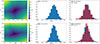 |
Fig. A.1. Results of the fitting to find the distribution of ηrad, analogous to Fig. 2. The top (bottom) row shows those obtained with a log10ηobs distribution de-trended from the correlation ∝ Ėβ, with β equal to −0.5 (−0.32). Both cases were obtained using the distance uncertainty distributed as P(Δ) = 𝒩 and with a Gaussian as the trial distribution. |
All Tables
Best-fitting parameters of the trial distributions of P(log10ηrad) for different distributions of distance uncertainty.
Best-fitting parameters of log10ηrad with P(log10ηrad) = 𝒩 and P(Δ) = 𝒩(0,0.341) for the distance uncertainty, considering the original log10ηobs distribution or the ones de-trended with the correlation ∝ Ėβ.
All Figures
|
Fig. 1. Probability density of the terms forming log10ηobs. Top: log10fΩ (left) and log10ϵI (right). Bottom: log10ϵd from different prescriptions, P(Δ) = 𝒩 (left) and P(ϵd) = 𝒩 (right). |
| In the text | |
|
Fig. 2. Results of the fitting to find the distribution of ηrad. The top (middle) row shows those obtained using the distance uncertainty distributed as P(Δ) = 𝒩, with a Gaussian (skew normal) as the trial distribution. The bottom row were obtained with the distance uncertainty distributed as P(ϵd) = 𝒩, with a Gaussian as the trial distribution. From left to right: contour plot of DKS in the space of parameters μrad − σrad (in the skew normal case we collapsed all the contours for the different α considered taking the smallest DKS for each pair μrad − σrad), best-fitting distribution of log10ηrad, overlapped distribution of log10ηobs (red), and joint distribution (blue). |
| In the text | |
|
Fig. A.1. Results of the fitting to find the distribution of ηrad, analogous to Fig. 2. The top (bottom) row shows those obtained with a log10ηobs distribution de-trended from the correlation ∝ Ėβ, with β equal to −0.5 (−0.32). Both cases were obtained using the distance uncertainty distributed as P(Δ) = 𝒩 and with a Gaussian as the trial distribution. |
| In the text | |
Current usage metrics show cumulative count of Article Views (full-text article views including HTML views, PDF and ePub downloads, according to the available data) and Abstracts Views on Vision4Press platform.
Data correspond to usage on the plateform after 2015. The current usage metrics is available 48-96 hours after online publication and is updated daily on week days.
Initial download of the metrics may take a while.