| Issue |
A&A
Volume 704, December 2025
|
|
|---|---|---|
| Article Number | A45 | |
| Number of page(s) | 8 | |
| Section | Galactic structure, stellar clusters and populations | |
| DOI | https://doi.org/10.1051/0004-6361/202557691 | |
| Published online | 01 December 2025 | |
Fluorine evolution in the Galactic halo
1
INAF, Osservatorio Astronomico di Trieste,
via G.B. Tiepolo 11,
34131
Trieste,
Italy
2
IFPU, Institute for Fundamental Physics of the Universe,
Via Beirut 2,
34151
Trieste,
Italy
3
Heidelberger Institut für Theoretische Studien,
Schloss-Wolfsbrunnenweg 35,
69118
Heidelberg,
Germany
4
INFN, Sezione di Trieste,
via Valerio 2,
34134
Trieste,
Italy
5
Dipartimento di Fisica, Sezione di Astronomia, Università di Trieste,
Via G. B. Tiepolo 11,
34143
Trieste,
Italy
★ Corresponding author: This email address is being protected from spambots. You need JavaScript enabled to view it.
Received:
14
October
2025
Accepted:
30
October
2025
Abstract
Context. The chemical evolution of fluorine is still a matter of debate in Galactic archaeology, especially at low metallicities, where it is particularly challenging to obtain the corresponding chemical abundances from observations.
Aims. We present here the first detailed theoretical study of the chemical evolution of fluorine at low metallicities using a stochastic chemical evolution model for the Galactic halo, in light of the most recent data for fluorine, which include observations at lower metallicities down to [Fe/H]∼ −4 dex, more than a factor of 10 lower than previous detections.
Methods. We employed a state-of-the-art stochastic chemical evolution model to follow the evolution in the Galactic halo, which has been shown to reproduce the main observables in this Galactic component and the abundance patterns of CNO and neutron-capture elements, and we implemented nucleosynthesis prescriptions for fluorine, focusing on the chemical evolution of this element.
Results. By comparing recent observations with model predictions, we confirm the importance of rotating massive stars at low metallicities to explain both the [F/Fe] versus [Fe/H] and [F/O] versus [O/H] diagrams. In particular, we show that we can reach a high [F/Fe] of ∼2 dex at an [Fe/H] of approximately −4 dex, in agreement with recent observations at the lowest metallicities.
Conclusions. With a stochastic chemical evolution model for the Galactic halo, we confirm the importance of rotating massive stars as fluorine producers, as suggested in previous studies that used chemical evolution models for the Galactic disc. We also expect an important production of F at high redshifts, in agreement with recent detections of super-solar N by JWST. Further data for fluorine at low metallicities, and also at high redshifts, are needed to put further constraints on the chemical evolution of fluorine and for comparison with our theoretical predictions.
Key words: Galaxy: abundances / Galaxy: evolution / Galaxy: formation
© The Authors 2025
 Open Access article, published by EDP Sciences, under the terms of the Creative Commons Attribution License (https://creativecommons.org/licenses/by/4.0), which permits unrestricted use, distribution, and reproduction in any medium, provided the original work is properly cited.
This article is published in open access under the Subscribe to Open model. This email address is being protected from spambots. You need JavaScript enabled to view it. to support open access publication.
1 Introduction
The origin and evolution of fluorine is still a matter of debate in the field of Galactic archaeology (see e.g. Ryde 2020), especially in the early stages of chemical enrichment in the Universe (Ryde & Harper 2021). Fluorine is very fragile and has only one stable isotope, 19F. In the literature, several stellar sites have been proposed for the production of fluorine: (i) thermal pulses in asymptotic giant branch (AGB) stars (Forestini et al. 1992; Jorissen et al. 1992; Straniero et al. 2006; Abia et al. 2011; Gallino et al. 2010; Karakas 2010; Cristallo et al. 2014), (ii) Wolf-Rayet (WR) stars (Meynet & Arnould 2000), (iii) rotating massive stars (Limongi & Chieffi 2018; Prantzos et al. 2018), (iv) the neutrino-process in core-collapse supernovae (CCSNe; Woosley & Haxton 1988; Kobayashi et al. 2011a), and (v) novae (José & Hernanz 1998).
In the literature, Galactic chemical evolution (GCE) models have been widely used to study the evolution of fluorine in the Milky Way and the role of the different fluorine producers (Timmes et al. 1995; Meynet & Arnould 2000; Renda et al. 2004; Kobayashi et al. 2011b; Prantzos et al. 2018; Spitoni et al. 2018; Olive & Vangioni 2019; Grisoni et al. 2020; Womack et al. 2023). Timmes et al. (1995) showed that, in principle, the ν-process could provide a possible explanation for the origin of fluorine, even if their yields of fluorine from CCSNe, including the ν-process, were not enough to reproduce the observational data. Meynet & Arnould (2000) suggested that WR stars can contribute significantly to the solar abundance of fluorine. Then, Renda et al. (2004) demonstrated quantitatively the impact of fluorine nucleosynthesis in WR and AGB stars, and the importance of the inclusion of these two fluorine production sites. However, the contribution of WR stars to the chemical evolution of fluorine was questioned in Palacios et al. (2005). Kobayashi et al. (2011b) found that the contribution of AGB stars to the chemical evolution of fluorine could only be seen at [Fe/H]> −1.5 dex, and it was not enough to reproduce the observations at [Fe/H] ~ 0 alone, so other fluorine sources were needed. In particular, Kobayashi et al. (2011a) showed that the ν-process of CCSNe and AGB stars combined together can contribute significantly to the production of fluorine: the main impact of the ν-process in the [F/O] versus [O/H] plot is represented by the presence of a plateau, followed by rapid increase due to AGB stars (see also Olive & Vangioni 2019). Moreover, novae have also been included in chemical evolution models that follow the evolution of fluorine; in particular, Spitoni et al. (2018) showed that novae can help better explain the observed secondary behaviour of fluorine in the [F/O] versus [O/H] diagram, even if their yields are very uncertain. Then, Prantzos et al. (2018) used the yields from rotating massive stars by Limongi & Chieffi (2018) in a GCE model, and they showed that this process can dominate fluorine production up to solar metallicities. Grisoni et al. (2020) focused on the chemical evolution of fluorine in the Galactic thick and thin discs in particular, and concluded that rotating massive stars are indeed important producers of F below [Fe/H]=−0.5 dex, although confirmation of its contribution for [Fe/H]< −1 required the extensive study of the Galactic halo that we present here. However, in order to reproduce the F abundance increase in the discs at late times, a contribution from lower-mass stars, such as single AGB stars and/or novae, is required. Later, Womack et al. (2023) also confirmed the importance of rotating massive stars in the chemical evolution of fluorine in the Milky Way, investigating the metallicity range −2<[Fe/H]<0.4. A detailed GCE study of fluorine in the metal-poor regime is still needed, as pointed out by Tsiatsiou et al. (2025), who present new results for the synthesis of F in massive stars with and without rotation, and state that GCE models that take the inhomogeneity of the interstellar medium (ISM) into consideration are needed to follow fluorine evolution in the Galactic halo. In particular, a detailed stochastic chemical evolution model, as presented in Rizzuti et al. (2025a), can also be applied to the study of the chemical evolution of fluorine in the Galactic halo in light of the most recent observational data, as we will show here.
In recent years, a great deal of work has been done on the chemical evolution of fluorine in the Galaxy with observational data (Abia et al. 2011, 2015, 2019; Recio-Blanco et al. 2012; de Laverny & Recio-Blanco 2013b,a; Jönsson et al. 2014; Pilachowski & Pace 2015; Guerço et al. 2019a,b; Ryde et al. 2020; Nandakumar et al. 2023; Brady et al. 2024; Bijavara Seshashayana et al. 2024a,b). Fluorine has been studied in open and globular clusters (Cunha et al. 2003; Cunha & Smith 2005; Smith et al. 2005; Yong et al. 2008; de Laverny & Recio-Blanco 2013b,a; Nault & Pilachowski 2013; Maiorca et al. 2014; Guerço et al. 2019b; Bijavara Seshashayana et al. 2024a,b). There have been studies of different Galactic components, such as the Galactic thick and thin discs (Guerço et al. 2019a; Ryde et al. 2020; Brady et al. 2024), the bulge (Jönsson et al. 2014), and the Galactic nuclear star cluster (Guerço et al. 2022). Recently, Nandakumar et al. (2023) studied in detail the evolution of fluorine at high metallicities (namely, −0.9 <[Fe/H] <0.25 dex) and recommended a set of vibrational-rotational HF lines to be used in the abundance analysis. However, the evolution of fluorine at low metallicities (e.g. [Fe/H] < −1.5 dex) poses a particular challenge due to the significant contamination from telluric lines and the blending of HF lines with CO features (Lucatello et al. 2011). Despite these difficulties, there are some measurements of fluorine abundances at low metallicities ([Fe/H] < −1.5 dex), such as in the works of Lucatello et al. (2011), Li et al. (2013), Abia et al. (2015), and Mura-Guzmán et al. (2020, 2025). In particular, the very recent work of Mura-Guzmán et al. (2025) presents F abundances and upper limits for seven stars, extending the lower metallicity limit for fluorine determination to [Fe/H]= −3.87 dex, which is more than a factor of 10 lower than previous detections. Finally, we note that fluorine has also been investigated at high redshifts. In particular, Franco et al. (2021) were able to estimate the abundance of fluorine in a gravitationally lensed galaxy at a redshift of z = 4.4, concluding that WR stars could be responsible for the observed fluorine abundance enhancement; this can also give important information about the origin of fluorine in the early Universe.
The aim of this paper is to model the evolution of fluorine in the Galactic halo using a stochastic chemical evolution model, as recently presented by Rizzuti et al. (2025a), and in light of the most recent data for fluorine at low metallicities (e.g. Mura-Guzmán et al. 2025).
Observational data used in this work: in the first column we report the source, in the second column the abundances used.
2 Observational data
In this work, we made use of recent data for fluorine in metal-poor regimes, complemented by data from the literature. In particular, we considered the recent work of Mura-Guzmán et al. (2025), who present F abundances and upper limits in seven carbon-enhanced metal-poor (CEMP) stars observed with the Immersion Grating Infrared Spectrometer (IGRINS; Yuk et al. 2010; Park et al. 2014; Mace et al. 2018), at the Gemini-South telescope. To complement this recent dataset, we also considered other results in the literature, for example F abundances and upper limits from Lucatello et al. (2011), who presented results for a sample of 11 metal-poor red giants. Their chemical abundances were obtained from an analysis of spectra from the CRyogenic high-resolution cross-dispersed InfraRed Echelle Spectrograph (CRIRES; Kaeufl et al. 2004) at the ESO Very Large Telescope (VLT). These stars are in the metallicity range −3.4<[Fe/H]<−1.3; fluorine measurements are available for two of them, and upper limits are available for the rest. We also considered Carina data from Abia et al. (2015); despite being observations of the Carina dwarf spheroidal (dSph) galaxy, they can give hints about the evolution of fluorine at low metallicities. All the observational data used in this work are summarized in Table 1.
3 Chemical evolution model
To follow the chemical evolution of fluorine in the Galactic halo, we adopted the stochastic chemical evolution code GEMS from Rizzuti et al. (2025a), where a detailed description of the model and the choice of parameters can be found.
3.1 The model
Rizzuti et al. (2025a) present a new version of the stochastic model first presented in Cescutti & Chiappini (2010), which was based on the original model of Cescutti (2008) and the homogeneous model of Chiappini et al. (2008). The GEMS code was specifically used to reproduce the chemical evolution of the Galactic halo; therefore, it runs for 1 Gyr after the formation of the Galaxy. To reproduce inhomogeneities in the chemical composition, stochasticity is introduced by dividing the simulation domain into various sub-volumes, each having the typical volume covered by a type II supernova (SN) explosion, and all are considered to be independent. In this study we considered a high number of volumes (1000, much higher than e.g. Cescutti 2008, where 100 volumes were considered); this was due to the parallelized computing of the GEMS code, which permitted an increase in the number of volumes. Further increasing the number of volumes would increase the coverage of rare events, but the high-probability areas predicted by the model would remain the same, and thus the results would remain robust.
Only one infall episode was assumed for the Galactic halo, accreting gas of primordial composition with a Gaussian distribution (see e.g. Chiappini et al. 2008):

where t0 is 100 Myr, τ is 50 Myr, the normalization is given by Σh=80 M⊙ pc−2, and A is the surface of each cell, so that ΣhA=3.2 × 10⁶ M⊙. The initial mass function (IMF) we used is from Scalo (1986), as in Rizzuti et al. (2025a). In Rizzuti et al. (2025a), they also tested the IMF from Kroupa (2001), which is more top-heavy than that from Scalo (1986); they show the results in their appendix (their Figs. C.1 and C.2), where the impact of the different IMF is shown to not be significant. The star formation rate (SFR) in units of M⊙ Gyr−1 was defined as:

where ν is 1.4 Gyr−1, k is 1.5, and Ggas(t) is the amount of gas within a volume of 1 M⊙. Finally, a Galactic wind that takes gas out of each cell was considered, with a rate proportional to star formation:

with a constant ω set to 8 for all chemical species (Chiappini et al. 2008). The evolution proceeds as follows. At each time step, in each cell a certain mass of gas according to the SFR is converted into stars, randomly extracted with a mass between 0.1 and 100 M⊙. Thus, each cell has the same amount of stars in terms of mass, but with a different distribution. After stars are born, their evolution is followed until they die, considering the stellar lifetimes from Maeder & Meynet (1989). Further details on the model prescriptions, and an exhaustive description of the model, are given in Rizzuti et al. (2025a).
3.2 Nucleosynthesis prescriptions
The nucleosynthesis prescriptions and the implementation of the yields in the model are fundamental ingredients for chemical evolution models. In this work, we implemented nucleosynthesis prescriptions following Rizzuti et al. (2025a), with the inclusion of fluorine.
For rotating massive stars, we used the yields of Limongi & Chieffi (2018, their recommended set, set R), who provide a grid of nine masses between 13 and 120 M⊙, four metallicities, [Fe/H]=0,−1,−2, and −3, and three rotations with initial equatorial velocities of 0 (non-rotating), 150, and 300 km s−1. This grid of models has been widely used in GCE studies (see e.g. Prantzos et al. 2018, 2023; Rizzuti et al. 2021; Romano et al. 2020, 2021; Grisoni et al. 2021; Kobayashi 2022; Rossi et al. 2024; Rizzuti et al. 2025a). There is still significant uncertainty in the explodability of massive stars, both observationally and theoretically. However, assumptions on the explosive mass range in our models have, in the past, allowed a good reproduction of the CNO and neutron-capture elements, as described in Rizzuti et al. (2025a). Therefore, in this study we also relied on these assumptions for the reproduction of F.
Following Rizzuti et al. (2025a), all massive stars were assumed to have the same rotation velocity, depending on their metallicity:
velocity([Fe/H]) = 300 km s−1 for [Fe/H] ≤ −3,
velocity([Fe/H]) = 150 km s−1 for [Fe/H] > −3.
This distribution was consistent with findings from Prantzos et al. (2018) and Rizzuti et al. (2019), with faster rotation in the early Galactic phases and slower in the subsequent ones (see also, Romano et al. 2020; Grisoni et al. 2021). Here, we were interested only in metal-poor stars ([Fe/H]< − 2), and therefore we did not decrease the rotation even further towards higher metallicities, as discussed, for example, in Rizzuti et al. (2021).
To reproduce observations for [Fe/H]< − 3 (the lowest metal-licity in the grid of stellar models of Limongi & Chieffi 2018), we considered the grid of Roberti et al. (2024), who also used the FRANEC code and provided 15 and 25 M⊙ models with [Fe/H]=−4, −5 and zero metals (Z=0) for a wide range of rotational velocities. Further details on these sets of yields for fluorine are given in the appendix.
Regarding the contribution from low- and intermediate-mass stars (LIMSs), the yields were taken from stellar models obtained from the FRUITY database for non-rotating stars between 1.3 and 6 M⊙ (Cristallo et al. 2009, 2011, 2015). However, their impact can only be visible in the model results from [Fe/H]>−2 dex. Finally, for Type Ia SNe , the yields were from Iwamoto et al. (1999), even if the contribution of Type Ia SNe to the fluorine budget was minimal.
4 Results
In Fig. 1, we show the observed and predicted [F/Fe] versus [Fe/H] for our reference model (left panel) and the non-rotating case (right panel). We immediately note the very different predictions from the two cases (rotating vs non-rotating) and, thus, the importance of rotating massive stars as fluorine producers. In particular, the model predictions for our reference model (left panel of Fig. 1) are from the stochastic chemical evolution model of the Galactic halo of Rizzuti et al. (2025a), with the inclusion of fluorine nucleosynthesis as described in Sect. 3. The model of Rizzuti et al. (2025a) has been shown to closely reproduce the main observables in this Galactic component and the abundance patterns of CNO and neutron-capture elements (see their Fig. 10 for their reference [O/Fe] vs. [Fe/H] diagram).
In the figure we compare our model predictions for fluorine with the data from Mura-Guzmán et al. (2025) and Lucatello et al. (2011). We furthermore show data from Abia et al. (2015); as previously mentioned, even if the data from Abia et al. (2015) are observations of the Carina dSph galaxy, they provide indications about the evolution of fluorine at low metallicities. As discussed in the introduction, there are many criticalities in the determination of fluorine abundances at low metallicities, and therefore many of the available data are only upper limits, as indicated by the arrows. While upper limits are not as certain as absolute determinations, they still inform us about the range of fluorine abundances that we should expect, and thus give us an idea of whether our predictions can match the observations. We also note that some stars in our sample are classified as CEMP-s (i.e. CEMP stars enriched in s-process elements). These stars likely had their surface fluorine abundances altered by binary mass transfer from an AGB companion, which changed the initial surface abundances (see Beers & Christlieb 2005; Lucatello et al. 2005; Bisterzo et al. 2010; Hansen et al. 2016). Therefore, for such stars, the predictions of our chemical evolution model can only provide a reference for the average fluorine abundances at birth in CEMP-s stars, before mass transfer took place. Further data are definitely needed to draw firm conclusions about fluorine evolution at lower metallicities. However, we highlight the novelty of our predictions in light of the most recent available data for fluorine; such new data, as in the very recent work of Mura-Guzmán et al. (2025), present the lowest metallicity limit in fluorine available to date.
At the lowest metallicities, the model predictions for our reference model, which includes rotating massive stars (left panel of Fig. 1), show a tail reaching relatively high [F/Fe] values ([F/Fe] of ∼2 dex at [Fe/H] of approximately −4 dex, in agreement with the lowest-metallicity F determination). The possibility of reaching such high [F/Fe] is due to the fact that rotating massive stars produce fluorine and small amounts of iron (see also [X/Fe] vs. [Fe/H] for CNO elements in Rizzuti et al. 2025a, their Fig. 10). In this way, rotating massive stars can set high values for [F/Fe] at low metallicities, in good agreement with the data. Rapidly rotating massive stars can produce primary fluorine from 14N through proton and alpha captures in the presence of 13C (Prantzos et al. 2018; Grisoni et al. 2020); 14N derives from reactions with 12C, which comes from He burning in the massive star itself and is thus of primary origin. This chain of reactions clearly also occurs in the non-rotating case, but the available amount of CNO nuclei is too small to contribute significantly to fluorine production (Limongi & Chieffi 2018).
We note that there are still no observations available for metallicities [Fe/H]<−4 dex. The lowest-metallicity data are the very recent determinations by Mura-Guzmán et al. (2025) for CS 29498-0043, a CEMP-no star at [Fe/H]= −3.87 with an F detection of [F/Fe] = +2.0 ± 0.4. This is the lowest-metallicity star with an observed F abundance to date, which we are able to explain with our stochastic chemical evolution model. For values −4<[Fe/H]<−2 dex, the model can reproduce the values for most stars, but we also note that we still have many upper limits.
Finally, for [Fe/H]>−2 dex, the contribution from LIMSs becomes important, but we do not extrapolate results from the model in this range since our model is mainly focused on the Galactic halo. However, Grisoni et al. (2020) studied fluorine in the thick and thin discs using GCE models specifically tailored to investigate the Galactic discs (Grisoni et al. 2017, 2018, 2019). They conclude that rotating massive stars are, indeed, important producers of F and can set high values in [F/Fe] abundance below [Fe/H]=−0.5 dex (in agreement with Prantzos et al. 2018; Womack et al. 2023). However, their contribution to [Fe/H]< −1 needed to be confirmed by an extensive study in the Galactic halo, which we present here. On the other hand, in order to reproduce the increase in F abundance in the discs at late times, a contribution from non-rotating massive stars, lower-mass stars, single AGB stars, and/or novae should be required (Spitoni et al. 2018; Grisoni et al. 2020; Womack et al. 2023).
In the right panel of Fig. 1, we show the case with non-rotating massive stars, and the difference is striking. We thus confirm the need for rotating massive stars to set high [F/Fe] values at low metallicities, something that is not present in the non-rotating case.
In Fig. 2, we then show the observed and predicted [F/O] versus [O/H], widely used in the literature to investigate the evolution of fluorine. In this way, we can remove the dependence on iron and use oxygen instead as a metallicity indicator. In this case also, rotating massive stars can set a plateau in [F/O] at lower metallicities, as suggested in previous studies of the Galactic disc (Grisoni et al. 2020; Womack et al. 2023). We see that the model predictions for our reference model (left panel) can reproduce the general trends of the data (and upper values), at variance with the non-rotating case (right panel), where it is not possible to explain observations. Thus, we confirm the importance of rotating massive stars as fluorine producers. Tsiatsiou et al. (2025, their Fig. 10) present a [F/O]-[O/H] relation computed with the CELIB code (Saitoh 2017; Hirai et al. 2021), showing a plateau at [O/H] < –2 driven by rotating Pop III yields. Our results are consistent with their findings, stressing the importance of rotation in setting a plateau at low [O/H].
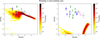 |
Fig. 1 Observed and predicted [F/Fe] vs. [Fe/H] for the Galactic halo for our reference chemical evolution model for variable rotational velocity as in Rizzuti et al. (2025a) (left) and for non-rotating massive stars (right). The data are taken from Mura-Guzmán et al. (2025) (blue) and Lucatello et al. (2011) (green), both upper limits and measurements with corresponding error bars; smaller dots correspond to CEMP-s stars. We also show Carina data from Abia et al. (2015) (magenta). |
5 Summary and conclusions
In this work we have studied the chemical evolution of fluorine, which is still a matter of debate in Galactic archaeology, especially at low metallicities. To this end, we present the first theoretical study of the chemical evolution of fluorine at low metallicities, using a state-of-the-art stochastic chemical evolution model (Rizzuti et al. 2025a), in light of the most recent data for fluorine at low metallicities (Mura-Guzmán et al. 2025).
Our main results can be summarized as follows.
With our stochastic chemical evolution model for the Galactic halo, we investigated fluorine evolution and the contribution of rapidly rotating massive stars using the yields of Limongi & Chieffi (2018) and Roberti et al. (2024).
With this set of nucleosynthesis prescriptions including variable rotational velocity, it is possible to reach high [F/Fe] values of ∼2 dex at [Fe/H] of approximately −4 dex, in agreement with very recent observations from Mura-Guzmán et al. (2025), who pushed observations to metallicities as low as [Fe/H]∼−4 dex; this is at variance with the non-rotating case where it is not possible to reach such high values.
We confirm that rotating massive stars can dominate fluorine production at such low metallicities (in agreement with suggestions from other studies, e.g. Prantzos et al. 2018; Grisoni et al. 2020; Womack et al. 2023).
We expect an important production of F also at high redshifts (see e.g. Franco et al. 2021), in agreement with recent detections of super-solar N by JWST (e.g. Cameron et al. 2023; Marques-Chaves et al. 2024), since F is produced in the same fashion by both AGB and rotating massive stars, as we show here (see also Kobayashi & Ferrara 2024; Rizzuti et al. 2025b).
To explain the secondary behaviour at higher metallicities ([Fe/H]>−2), other sites such as AGB stars and/or novae should be important (see e.g. Grisoni et al. 2020; Womack et al. 2023). However, we do not extrapolate results here since our model is tailored for the Galactic halo and not for the disc.
In conclusion, we confirm that rotating massive stars can be important producers of fluorine (Prantzos et al. 2018; Grisoni et al. 2020; Womack et al. 2023), and we show their impact on the chemical evolution of fluorine with a state-of-the-art chemical evolution model that accounts for inhomogeneities in the ISM. Further data at low metallicities and at high redshifts will be fundamental to further constrain the chemical evolution of fluorine.
Acknowledgements
We are grateful to the referee for all the useful comments and suggestions that improved our work. V.G. acknowledges financial support from the INAF program “Giovani Astrofisiche ed Astrofisici di Eccellenza -IAF: INAF Astrophysics Fellowships in Italy” (Project: GalacticA, “Galactic Archaeology: reconstructing the history of the Galaxy”) and from INAF Mini Grant 2023. F.R. is a fellow of the Alexander von Humboldt Foundation, and acknowledges support by the Klaus Tschira Foundation. F.R. also acknowledges I.N.A.F. for the 1.05.24.07.02 Mini grant 2024 “GALoMS - Galactic Archaeology for Low Mass Stars” (PI: C.T. Nguyen). F.R. and G.C. acknowledge financial support under the National Recovery and Resilience Plan (NRRP), Mission 4, Component 2, Investment 1.1, Call for tender No. 104 published on 2.2.2022 by the Italian Ministry of University and Research (MUR), 570 funded by the European Union - NextGenerationEU - Project ‘Cosmic POT’ (PI: L. Magrini) Grant Assignment Decree No. 2022X4TM3H by the Italian Ministry of Ministry of University and Research (MUR). G.C. thanks I.N.A.F. for the 1.05.23.01.09 Large Grant - Beyond metallicity: Exploiting the full POtential of CHemical elements (EPOCH) (ref. Laura Magrini) and the European Union’s Horizon 2020 research and innovation programme for the grant agreement No 101008324 (ChETEC-INFRA).
References
- Abia, C., Cunha, K., Cristallo, S., et al. 2011, ApJ, 737, L8 [Google Scholar]
- Abia, C., Cunha, K., Cristallo, S., & de Laverny, P. 2015, A&A, 581, A88 [NASA ADS] [CrossRef] [EDP Sciences] [Google Scholar]
- Abia, C., Cristallo, S., Cunha, K., de Laverny, P., & Smith, V. V. 2019, A&A, 625, A40 [CrossRef] [EDP Sciences] [Google Scholar]
- Beers, T. C., & Christlieb, N. 2005, ARA&A, 43, 531 [NASA ADS] [CrossRef] [Google Scholar]
- Bijavara Seshashayana, S., Jönsson, H., D’Orazi, V., et al. 2024a, A&A, 683, A218 [NASA ADS] [CrossRef] [EDP Sciences] [Google Scholar]
- Bijavara Seshashayana, S., Jönsson, H., D’Orazi, V., et al. 2024b, A&A, 689, A120 [NASA ADS] [CrossRef] [EDP Sciences] [Google Scholar]
- Bisterzo, S., Gallino, R., Straniero, O., Cristallo, S., & Käppeler, F. 2010, MNRAS, 404, 1529 [NASA ADS] [Google Scholar]
- Brady, K. E., Pilachowski, C. A., Grisoni, V., Maas, Z. G., & Nault, K. A. 2024, AJ, 167, 291 [Google Scholar]
- Cameron, A. J., Saxena, A., Bunker, A. J., et al. 2023, A&A, 677, A115 [NASA ADS] [CrossRef] [EDP Sciences] [Google Scholar]
- Cescutti, G. 2008, A&A, 481, 691 [NASA ADS] [CrossRef] [EDP Sciences] [Google Scholar]
- Cescutti, G., & Chiappini, C. 2010, A&A, 515, A102 [NASA ADS] [CrossRef] [EDP Sciences] [Google Scholar]
- Chiappini, C., Ekström, S., Meynet, G., et al. 2008, A&A, 479, L9 [NASA ADS] [CrossRef] [EDP Sciences] [Google Scholar]
- Cristallo, S., Straniero, O., Gallino, R., et al. 2009, ApJ, 696, 797 [NASA ADS] [CrossRef] [Google Scholar]
- Cristallo, S., Piersanti, L., Straniero, O., et al. 2011, ApJS, 197, 17 [NASA ADS] [CrossRef] [Google Scholar]
- Cristallo, S., Di Leva, A., Imbriani, G., et al. 2014, A&A, 570, A46 [CrossRef] [EDP Sciences] [Google Scholar]
- Cristallo, S., Straniero, O., Piersanti, L., & Gobrecht, D. 2015, ApJS, 219, 40 [Google Scholar]
- Cunha, K., & Smith, V. V. 2005, ApJ, 626, 425 [NASA ADS] [CrossRef] [Google Scholar]
- Cunha, K., Smith, V. V., Lambert, D. L., & Hinkle, K. H. 2003, AJ, 126, 1305 [NASA ADS] [CrossRef] [Google Scholar]
- de Laverny, P., & Recio-Blanco, A. 2013a, A&A, 555, A121 [NASA ADS] [CrossRef] [EDP Sciences] [Google Scholar]
- de Laverny, P., & Recio-Blanco, A. 2013b, A&A, 560, A74 [NASA ADS] [CrossRef] [EDP Sciences] [Google Scholar]
- Forestini, M., Goriely, S., Jorissen, A., & Arnould, M. 1992, A&A, 261, 157 [NASA ADS] [Google Scholar]
- Franco, M., Coppin, K. E. K., Geach, J. E., et al. 2021, Nat. Astron., 5, 1240 [Google Scholar]
- Gallino, R., Bisterzo, S., Cristallo, S., & Straniero, O. 2010, Mem. Soc. Astron. Italiana, 81, 998 [Google Scholar]
- Grisoni, V., Spitoni, E., Matteucci, F., et al. 2017, MNRAS, 472, 3637 [Google Scholar]
- Grisoni, V., Spitoni, E., & Matteucci, F. 2018, MNRAS, 481, 2570 [NASA ADS] [Google Scholar]
- Grisoni, V., Matteucci, F., Romano, D., & Fu, X. 2019, MNRAS, 489, 3539 [NASA ADS] [CrossRef] [Google Scholar]
- Grisoni, V., Romano, D., Spitoni, E., et al. 2020, MNRAS, 498, 1252 [NASA ADS] [CrossRef] [Google Scholar]
- Grisoni, V., Matteucci, F., & Romano, D. 2021, MNRAS, 508, 719 [NASA ADS] [CrossRef] [Google Scholar]
- Guerço, R., Cunha, K., Smith, V. V., et al. 2019a, ApJ, 885, 139 [Google Scholar]
- Guerço, R., Cunha, K., Smith, V. V., et al. 2019b, ApJ, 876, 43 [Google Scholar]
- Guerço, R., Ramírez, S., Cunha, K., et al. 2022, ApJ, 929, 24 [CrossRef] [Google Scholar]
- Hansen, T. T., Andersen, J., Nordström, B., et al. 2016, A&A, 588, A3 [NASA ADS] [CrossRef] [EDP Sciences] [Google Scholar]
- Hirai, Y., Fujii, M. S., & Saitoh, T. R. 2021, PASJ, 73, 1036 [NASA ADS] [CrossRef] [Google Scholar]
- Iwamoto, K., Brachwitz, F., Nomoto, K., et al. 1999, ApJS, 125, 439 [NASA ADS] [CrossRef] [Google Scholar]
- Jönsson, H., Ryde, N., Harper, G. M., et al. 2014, A&A, 564, A122 [NASA ADS] [CrossRef] [EDP Sciences] [Google Scholar]
- Jorissen, A., Smith, V. V., & Lambert, D. L. 1992, A&A, 261, 164 [NASA ADS] [Google Scholar]
- José, J., & Hernanz, M. 1998, ApJ, 494, 680 [Google Scholar]
- Kaeufl, H.-U., Ballester, P., Biereichel, P., et al. 2004, SPIE Conf. Ser., 5492, 1218 [NASA ADS] [Google Scholar]
- Karakas, A. I. 2010, MNRAS, 403, 1413 [NASA ADS] [CrossRef] [Google Scholar]
- Kobayashi, C. 2022, IAU Symp., 366, 63 [Google Scholar]
- Kobayashi, C., & Ferrara, A. 2024, ApJ, 962, L6 [NASA ADS] [CrossRef] [Google Scholar]
- Kobayashi, C., Izutani, N., Karakas, A. I., et al. 2011a, ApJ, 739, L57 [Google Scholar]
- Kobayashi, C., Karakas, A. I., & Umeda, H. 2011b, MNRAS, 414, 3231 [NASA ADS] [CrossRef] [Google Scholar]
- Kroupa, P. 2001, MNRAS, 322, 231 [NASA ADS] [CrossRef] [Google Scholar]
- Li, H. N., Ludwig, H. G., Caffau, E., Christlieb, N., & Zhao, G. 2013, ApJ, 765, 51 [NASA ADS] [CrossRef] [Google Scholar]
- Limongi, M., & Chieffi, A. 2018, ApJS, 237, 13 [NASA ADS] [CrossRef] [Google Scholar]
- Lucatello, S., Tsangarides, S., Beers, T. C., et al. 2005, ApJ, 625, 825 [NASA ADS] [CrossRef] [Google Scholar]
- Lucatello, S., Masseron, T., Johnson, J. A., Pignatari, M., & Herwig, F. 2011, ApJ, 729, 40 [CrossRef] [Google Scholar]
- Mace, G., Sokal, K., Lee, J.-J., et al. 2018, SPIE Conf. Ser., 10702, 107020Q [NASA ADS] [Google Scholar]
- Maeder, A., & Meynet, G. 1989, A&A, 210, 155 [Google Scholar]
- Maiorca, E., Uitenbroek, H., Uttenthaler, S., et al. 2014, ApJ, 788, 149 [NASA ADS] [CrossRef] [Google Scholar]
- Marques-Chaves, R., Schaerer, D., Kuruvanthodi, A., et al. 2024, A&A, 681, A30 [NASA ADS] [CrossRef] [EDP Sciences] [Google Scholar]
- Meynet, G., & Arnould, M. 2000, A&A, 355, 176 [NASA ADS] [Google Scholar]
- Mura-Guzmán, A., Yong, D., Abate, C., et al. 2020, MNRAS, 498, 3549 [CrossRef] [Google Scholar]
- Mura-Guzmán, A., Yong, D., Kobayashi, C., et al. 2025, MNRAS, 538, 3177 [Google Scholar]
- Nandakumar, G., Ryde, N., & Mace, G. 2023, A&A, 676, A79 [NASA ADS] [CrossRef] [EDP Sciences] [Google Scholar]
- Nault, K. A., & Pilachowski, C. A. 2013, AJ, 146, 153 [NASA ADS] [CrossRef] [Google Scholar]
- Olive, K. A., & Vangioni, E. 2019, MNRAS, 490, 4307 [CrossRef] [Google Scholar]
- Palacios, A., Arnould, M., & Meynet, G. 2005, A&A, 443, 243 [NASA ADS] [CrossRef] [EDP Sciences] [Google Scholar]
- Park, C., Jaffe, D. T., Yuk, I.-S., et al. 2014, SPIE Conf. Ser., 9147, 91471D [NASA ADS] [Google Scholar]
- Pilachowski, C. A., & Pace, C. 2015, AJ, 150, 66 [NASA ADS] [CrossRef] [Google Scholar]
- Prantzos, N., Abia, C., Limongi, M., Chieffi, A., & Cristallo, S. 2018, MNRAS, 476, 3432 [Google Scholar]
- Prantzos, N., Abia, C., Chen, T., et al. 2023, MNRAS, 523, 2126 [NASA ADS] [CrossRef] [Google Scholar]
- Recio-Blanco, A., de Laverny, P., Worley, C., et al. 2012, A&A, 538, A117 [NASA ADS] [CrossRef] [EDP Sciences] [Google Scholar]
- Renda, A., Fenner, Y., Gibson, B. K., et al. 2004, MNRAS, 354, 575 [NASA ADS] [CrossRef] [Google Scholar]
- Rizzuti, F., Cescutti, G., Matteucci, F., et al. 2019, MNRAS, 489, 5244 [NASA ADS] [Google Scholar]
- Rizzuti, F., Cescutti, G., Matteucci, F., et al. 2021, MNRAS, 502, 2495 [NASA ADS] [CrossRef] [Google Scholar]
- Rizzuti, F., Cescutti, G., Molaro, P., et al. 2025a, A&A, 698, A118 [NASA ADS] [CrossRef] [EDP Sciences] [Google Scholar]
- Rizzuti, F., Matteucci, F., Molaro, P., Cescutti, G., & Maiolino, R. 2025b, A&A, 697, A96 [NASA ADS] [CrossRef] [EDP Sciences] [Google Scholar]
- Roberti, L., Limongi, M., & Chieffi, A. 2024, ApJS, 270, 28 [NASA ADS] [CrossRef] [Google Scholar]
- Romano, D., Franchini, M., Grisoni, V., et al. 2020, A&A, 639, A37 [NASA ADS] [CrossRef] [EDP Sciences] [Google Scholar]
- Romano, D., Magrini, L., Randich, S., et al. 2021, A&A, 653, A72 [NASA ADS] [CrossRef] [EDP Sciences] [Google Scholar]
- Rossi, M., Romano, D., Mucciarelli, A., et al. 2024, A&A, 691, A284 [NASA ADS] [CrossRef] [EDP Sciences] [Google Scholar]
- Ryde, N. 2020, J. Astrophys. Astron., 41, 34 [NASA ADS] [CrossRef] [Google Scholar]
- Ryde, N., & Harper, G. 2021, Nat. Astron., 5, 1212 [Google Scholar]
- Ryde, N., Jönsson, H., Mace, G., et al. 2020, ApJ, 893, 37 [CrossRef] [Google Scholar]
- Saitoh, T. R. 2017, AJ, 153, 85 [NASA ADS] [CrossRef] [Google Scholar]
- Scalo, J. M. 1986, Fund. Cosmic Phys., 11, 1 [NASA ADS] [EDP Sciences] [Google Scholar]
- Smith, V. V., Cunha, K., Ivans, I. I., et al. 2005, ApJ, 633, 392 [Google Scholar]
- Spitoni, E., Matteucci, F., Jönsson, H., Ryde, N., & Romano, D. 2018, A&A, 612, A16 [NASA ADS] [CrossRef] [EDP Sciences] [Google Scholar]
- Straniero, O., Gallino, R., & Cristallo, S. 2006, Nucl. Phys. A, 777, 311 [NASA ADS] [CrossRef] [Google Scholar]
- Timmes, F. X., Woosley, S. E., & Weaver, T. A. 1995, ApJS, 98, 617 [NASA ADS] [CrossRef] [Google Scholar]
- Tsiatsiou, S., Meynet, G., Farrell, E., et al. 2025, A&A, 696, A241 [NASA ADS] [CrossRef] [EDP Sciences] [Google Scholar]
- Womack, K. A., Vincenzo, F., Gibson, B. K., et al. 2023, MNRAS, 518, 1543 [Google Scholar]
- Woosley, S. E., & Haxton, W. C. 1988, Nature, 334, 45 [NASA ADS] [CrossRef] [Google Scholar]
- Yong, D., Meléndez, J., Cunha, K., et al. 2008, ApJ, 689, 1020 [NASA ADS] [CrossRef] [Google Scholar]
- Yuk, I.-S., Jaffe, D. T., Barnes, S., et al. 2010, SPIE Conf. Ser., 7735, 77351M [NASA ADS] [Google Scholar]
Appendix A Stellar yields
Here we discuss the stellar yields of fluorine from Limongi & Chieffi (2018) and Roberti et al. (2024), which have been included in our chemical evolution model for the Galactic halo. As mentioned in Sect. 3, Limongi & Chieffi (2018) have presented a set of yields for different mass, metallicity, and rotational velocity.
In Fig. A.1 we show the fluorine yields in the stellar models of Limongi & Chieffi (2018) (left column) and only wind (right column), for three initial velocities: 0 km/s (upper panels), 150 km/s (middle panels) and 300 km/s (lower panels), set R and total yields. In particular, it is evident that fluorine is mostly produced by 13-25 M⊙ at high rotational velocities (150-300 km/s). Those are the same stars that undergo SN explosion in the set R. In Sect. 3 we also discussed that a new set of FRANEC models has been published by Roberti et al. (2024), for 15 and 25 M⊙ stars with metallicity [Fe/H]=-4,-5, and zero metals (Z=0) for various rotational velocities. Even if the mass range is small, the very low metallicity and large rotational velocity range make this grid a perfect tool for investigating the nucleosynthesis of the first stars (see Rizzuti et al. 2025a). In Fig. A.2, we show the fluorine yields as predicted by the models of Roberti et al. (2024) as a function of the stellar initial equatorial velocity. From Fig. A.2, it is evident that fluorine generally increases with rotation, perfectly in agreement with our assumption of velocity function and Limongi & Chieffi (2018).
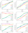 |
Fig. A.1 Fluorine total yields in the stellar models of Limongi & Chieffi (2018) (left column) and only wind (right column), for three initial rotational velocities: 0 km/s (upper panels), 150 km/s (middle panels), and 300 km/s (lower panels). |
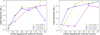 |
Fig. A.2 Fluorine yields in the stellar models of Roberti et al. (2024) for 15 (left) and 25 M⊙ (right) stars, as a function of the star initial equatorial velocity in km/s. Different colors correspond to different metallicities: [Fe/H]=-4, -5, and −∞ (zero metals). |
All Tables
Observational data used in this work: in the first column we report the source, in the second column the abundances used.
All Figures
|
Fig. 1 Observed and predicted [F/Fe] vs. [Fe/H] for the Galactic halo for our reference chemical evolution model for variable rotational velocity as in Rizzuti et al. (2025a) (left) and for non-rotating massive stars (right). The data are taken from Mura-Guzmán et al. (2025) (blue) and Lucatello et al. (2011) (green), both upper limits and measurements with corresponding error bars; smaller dots correspond to CEMP-s stars. We also show Carina data from Abia et al. (2015) (magenta). |
| In the text | |
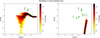 |
Fig. 2 Same as Fig. 1 but for [F/O] vs. [O/H]. |
| In the text | |
|
Fig. A.1 Fluorine total yields in the stellar models of Limongi & Chieffi (2018) (left column) and only wind (right column), for three initial rotational velocities: 0 km/s (upper panels), 150 km/s (middle panels), and 300 km/s (lower panels). |
| In the text | |
|
Fig. A.2 Fluorine yields in the stellar models of Roberti et al. (2024) for 15 (left) and 25 M⊙ (right) stars, as a function of the star initial equatorial velocity in km/s. Different colors correspond to different metallicities: [Fe/H]=-4, -5, and −∞ (zero metals). |
| In the text | |
Current usage metrics show cumulative count of Article Views (full-text article views including HTML views, PDF and ePub downloads, according to the available data) and Abstracts Views on Vision4Press platform.
Data correspond to usage on the plateform after 2015. The current usage metrics is available 48-96 hours after online publication and is updated daily on week days.
Initial download of the metrics may take a while.