© The Authors 2025

1. Introduction

A high-mass microquasar (HMMQ) is composed of a black hole (BH) and a massive companion star. A jet bursting out of a HMMQ behaves as a scaled-down jet in an active galactic nucleus (AGN) (López-Miralles et al. 2022), except the former jet is blown by powerful wind from the massive companion star. A jet from a HMMQ evolves much more quickly than its counterpart in an AGN, making the former valuable in studying the accretion, eruption, and emission processes around a black hole.

Relativistic jets were conjectured to play an important role in the γ-ray emission from HMMQs (Zanin et al. 2016), possibly via inverse Compton scattering on stellar photons and disk photons. The dynamics of jet–wind interaction and relevant radiation mechanisms can be simulated to reveal more details that are not available in observation.

Cygnus X-1, one of the brightest X-ray sources in the sky, is a high-mass microquasar located at 2.22 kpc from the Earth (Zanin et al. 2016; Miller-Jones et al. 2021). The spectrum of Cygnus X-1, ranging from 0.1 keV to hundreds of GeV, has been observed with several telescopes, for example BeppoSAX, MAGIC, Fermi-LAT, AGILE, and INTEGRAL (Salvo et al. 2001; Albert et al. 2007; Malyshev et al. 2013; Sabatini et al. 2013; Rodriguez et al. 2015; Zanin et al. 2016). The spectrum of Cygnus X-1 manifests a combination of a blackbody-like spectrum attributed to the accretion disk and a power-law spectrum.

Two spectral states were identified in the spectrum of Cygnus X-1 (Salvo et al. 2001; Zdziarski & Gierliński 2004; Zanin et al. 2016). In the soft state, the spectrum is dominated by thermal emission with a peak at kT ≃ 1 keV, followed by a power-law tail up to 10 MeV, with photon index Γ ≃ 2–3. In the hard state, the blackbody-like emission is less luminous, with a peak at kT ≃ 0.1 keV. Most emission follows a power-law spectrum up to hundreds of keV, with a photon index Γ ≃ 1.5. In addition, a steady emission with photon index Γ ≃ 2.5 up to 20 GeV was detected in the hard state (Malyshev et al. 2013; Zanin et al. 2016).

The X-ray emission from Cygnus X-1 is mostly attributed to the disk photons via inverse Compton scattering by the hot thermal electrons in the inner accretion flow (Shapiro et al. 1976). However, a nonthermal emission model suggested that particles could be accelerated to relativistic energy and could emit persistent GHz radio signals (Akharonian & Vardanian 1985). The radio signals were found to be similar to the X-ray emissions from X-ray binaries, suggesting that plasma jets might play an important role in X-ray emissions (Markoff et al. 2003; Gallo et al. 2012).

Gigaelectronvolt emissions from Cygnus X-1 have been detected with the telescopes of MAGIC, AGILE, and Fermi-LAT (Albert et al. 2007; Malyshev et al. 2013; Zanin et al. 2016). In Malyshev et al. (2013), steady emission of high-energy γ-rays from Cygnus X-1 was detected in 0.03–300 GeV, with a photon index Γ = 2.6 ± 0.2. In Zanin et al. (2016), 7.5 years of data collected by the Fermi-LAT were analyzed to study the high-energy (> 60 MeV) emission from Cygnus X-1. The luminosity is about 5.5 × 10³³ erg/s, and the emission source was estimated to lie between 10¹¹ and 10¹³ cm from the black hole, manifesting flux orbital variability. The photon index of the high-energy emission was Γ = 2.3 ± 0.2, slightly smaller than that derived in Malyshev et al. (2013).

The interactions among the relativistic jet, stellar wind, and magnetic field are intricate, making the observed features difficult to interpret. Numerical simulations can be applied to a variety of scenarios to help interpret the observed phenomena.

In Perucho et al. (2010), the dynamics of a hot jet (at a temperature of 10¹⁰ K) traversing a stellar wind was simulated by using a hydrodynamics (HD) model. The difference in evolution characteristics between dilute and dense jets was studied.

In de la Cita et al. (2016, 2017), the interaction between the stellar wind and relativistic jet was simulated with a relativistic hydrodynamics (RHD) model. The plasma dynamics and emission features of either an AGN or a HMMQ can be simulated by properly adjusting the normalization factors. Although an AGN is much larger than a HMMQ, the two jets have features that are similar in many aspects (de la Cita et al. 2016). In de la Cita et al. (2017), the interaction between a stellar wind and a clump-jet in a HMMQ was simulated. The high-energy emission at the GeV level via synchrotron radiation and inverse Compton scattering was computed in terms of the simulated plasma distribution, with the magnetic field perpendicular to the plasma flow.

In López-Miralles et al. (2022), a three-dimensional relativistic magnetohydrodynamics (RMHD) model was applied to simulate magnetized jets in high-mass X-ray binaries (HMXRBs), immersed in clumpy stellar winds and toroidal magnetic fields. The emission via synchrotron radiation and inverse Compton scattering was analyzed, under the approximation of frozen-in magnetic field and plasma flow with fixed β.

In Papavasileiou et al. (2023), an analytical model was proposed to study the γ-ray emission and absorption of three X-ray binary (XRB) systems, including Cygnus X-1. Part of the γ-rays emitted from the jet were absorbed by soft X-rays emitted from the accretion disk, hard X-rays emitted from the corona of the black hole, and thermal radiation from the donor star. The absorption by the donor star manifested flux orbital variability (Böttcher & Dermer 2005).

It was reported in Papavasileiou et al. (2023) that the absorption of γ-rays by soft X-rays emitted from the accretion disk dominated in the region of z < 10¹⁰ cm, where the black hole was located at the origin, the jet traveled in the z direction, and the donor star moved on the xy plane. The absorption by thermal radiation from the donor star dominated in the region of 10¹⁰ < z < 10¹² cm, while that by the black hole corona emission was insignificant.

Since the magnetic field significantly affects the evolution of jet–wind interaction, a self-consistent RMHD model that incorporates the interactions among the relativistic jet, stellar wind, and magnetic field will be very useful in explaining many observed features and predicting more complicated scenarios in the future. For this work, a 3D RMHD model was applied to simulate the plasma dynamics in a HMMQ, incorporating such interactions. The high-energy emissions out of the jet–wind interaction via synchrotron radiation and inverse Compton scattering are derived by taking a post-processing approach. The radiation mechanisms, spectrum, photon index, and flux orbital variability of the jet–wind interaction are investigated. The γ-ray absorption via the γ + γ → e⁺ + e⁻ process and the loss of nonthermal particles are taken into account.

The rest of this work is organized as follows. The physical models of RMHD, jet and stellar wind, nonthermal emission, and absorption are presented in Section 2. The simulation results of the jet–wind interaction, relevant emissions, absorption, radiation map, and spectra are discussed in Section 3. Our conclusions are drawn in Section 4.

2. Physical models

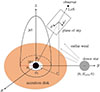Fig. 1. Schematic of a relativistic magnetized jet erupting from a HMMQ.

Figure 1 shows the schematic a relativistic magnetized jet erupting from a HMMQ. The simulations were conducted to study the plasma dynamics and high-energy emissions of these events. The relevant parameters were estimated from the observation data of Cygnus X-1, and hence the simulation results are useful in order to interpret some of its observed phenomena. The simulations focus on length scale of about 10¹¹–10¹² cm, which fits the γ-ray emitting region estimated in Zanin et al. (2016). Some detailed features such as the inner region and the eruption of the jet could not be revealed in the simulations.

The black hole is located at the origin, and the donor star rotates about the black hole with orbit radius of R_orb = 0.244 au = 3.66 × 10¹² cm (Miller-Jones et al. 2021). Affected by the stellar wind blown radially from the companion star (donor star), the jet radius is set to R_j = 6 × 10⁹ cm in the simulations (López-Miralles et al. 2022). Since the simulation time window is about 50 s, much shorter than the orbital period of 5.6 days (Reid et al. 2011; Miller-Jones et al. 2021), the donor star is approximately fixed in the simulations.

The computational domain is adopted as −50R_j < x, y < 50R_j and z₀ < z < z₀ + 120R_j, with z₀ = 6 × 10¹⁰ cm (López-Miralles et al. 2022). The viewing angle between the line of sight (LoS) and the plasma flow is θ_i = 27.5° (Miller-Jones et al. 2021). The LoS to the Earth bears an azimuth angle ϕ_i with respect to the x-axis. The x′- and y′-axes are the projection of x- and y-axes, respectively, onto the plane of the sky. We note that z₀ is much larger than the Schwarzschild radius of the black hole, and hence the effect of general relativity is ignored.

The plasma variables and the magnetic field are normalized with respect to R_j in length, c in speed, t₀ = R_j/c in time, ρ₀ = 2.8 × 10⁻¹⁵ g/cm³ in mass density, n₀ = ρ₀/m_p cm⁻³ in number density (where m_p = 1.67 × 10⁻²⁴ g is proton mass), p₀ = ρ₀c² erg/cm³ in pressure, e₀ = p₀ in energy density, and $b_0=\sqrt{4\pi {\rho }_0{c}^2}$ gauss in magnetic field.

The normalized RMHD equations governing the interactions between relativistic magnetized jet and stellar wind are given by (Chang & Kiang 2023, 2024)

$$\begin{array}{cc}\hfill {\partial }_{\mu }\left(\rho u^{\mu }\right)& =0,\hfill \end{array}$$(1)

$$\begin{array}{cc}\hfill {\partial }_{\nu }{T}^{\mu \nu }& =0,\hfill \end{array}$$(2)

$$\begin{array}{cc}\hfill {\partial }_{\nu }{G}^{\mu \nu }& =0,\hfill \end{array}$$(3)

where u^μ is the four velocity, T^μν = (ρ + ε + p + |b|²)u^μu^ν + (p + |b|²/2)g^μν − b^μb^ν is the stress-energy tensor, G^μν is the dual of Faraday tensor, ρ is the rest-mass density, ε is the internal energy density, p is the gas pressure, and b^μ is the magnetic four-vector. The gas pressure and the internal energy density satisfy the state equation p = ε(Γ_a − 1), with the adiabatic index Γ_a = 4/3.

In-house MATLAB codes were developed to solve the RMHD equations by using a Godunov-type finite-volume algorithm with HLL-type Riemann solvers and slope limiters (Toro 2009). A constrained transport method was applied to ensure the magnetic field satisfy the divergence-free condition (Londrillo & Del Zanna 2004), and the time step Δt was determined by the Courant-Friederichs-Lewy (CFL) condition to ensure the stability of simulations (Mignone & Bodo 2006). The codes were validated with shock tubes, Orzag-Tang and blast wave tests, and were used to simulate the evolution of relativistic magnetized jets (Chang & Kiang 2023, 2024). In Chang & Kiang (2023), simulations were conducted over an extensive set of parameters, including temperature, magnetization, and magnetic pitch angle. In Chang & Kiang (2024), nonthermal emissions, including synchrotron radiation, inverse Compton scattering and bremsstrahlung, were computed by using the plasma variables of the simulated jet.

For this work, the codes were modified to simulate the jet–wind interactions in a HMMQ and the accompanying radiation spectrum. The computational domain was segmented into a uniform grid of 400 × 400 × 480 voxels, at grid sizes of Δx = Δy = Δz = 0.25. The simulation results are very close to those obtained with coarse grid sizes of Δx = Δy = Δz = 1, confirming numerical convergence.

2.1. Models of jet and stellar wind

The computational domain is initially permeated with stellar wind blown from the donor star, and a relativistic magnetized jet is continuously erupted from the bottom of the computational domain. In Tetarenko et al. (2019), the flux variabilities of compact jet emissions observed in multiband radio and X-rays were analyzed. The jet emission at radio bands of 9 GHz and 11 GHz manifest high correlation on timescales associated with Fourier frequencies of f < 0.005 Hz, and no significant radio jet emission was observed at f > 0.03 Hz. The duration of jet eruption is set to 50 s to cover the Fourier frequencies manifesting significant radio emission. During this period, the jet traverses about 10¹² cm, consistent with the size of emission region estimated by Zanin et al. (2016).

The clumped structures in stellar wind were observed (Sundqvist et al. 2018; El Mellah et al. 2017). Inhomogeneous and clumped structures, featuring the line-deshadowing instability (LDI), were induced by the stellar winds blown from hot and massive stars (Sundqvist et al. 2018).

In Sundqvist et al. (2018), wind structures under the LDI mechanism were simulated. A shell structure was formed in the initial stage; then the plasma broke up into complex structures in density and velocity, manifesting small-scale clumps. The fully developed clumps were statistically isotropic, with a typical size of about 0.01R_* at 2R_*, where R_* is the stellar radius. In El Mellah et al. (2017), clumps were included in a nonstationary wind to evaluate the time-varying accretion process in X-ray binaries. The impact of clumps on the time variability of intrinsic mass accretion rate is severely tempered by the impinging shock from a companion star.

In López-Miralles et al. (2022), a clumpy stellar wind was included in the simulations of jet–wind interaction in high-mass X-ray binaries. The overall morphology and dynamics of jet were dominated by the amount of magnetic, kinetic, and thermal energies. The difference attributed to clumps was insignificant.

For this work, a homogeneous isotropic wind was adopted in modeling the jet–wind interaction, similar to previous works of jet–wind interaction (Perucho et al. 2010; de la Cita et al. 2016). The effect of an inhomogeneous clumped structure is neglected because the length scale of simulations is about two orders of magnitude larger than that of clumps (Sundqvist et al. 2018). In addition, the effects of clumpy wind on the dynamics of jet–wind interaction are insignificant and are easily smeared out by shock waves (López-Miralles et al. 2022; El Mellah et al. 2017). The proposed approach incorporates the interactions among the relativistic jet, stellar wind, and magnetic field, and will be very useful in explaining many observed features and predicting more complicated scenarios in the future.

The loss rate of mass in the donor star is about Ṁ_w = 10⁻⁶ M_⊙/yr, and the temperature of the stellar wind is about T = 10⁴ K (Perucho & Bosch-Ramon 2008; López-Miralles et al. 2022). Thus, the mass density ρ_w, gas pressure p_w and radial velocity v_w of the stellar wind are approximated as

$$\begin{array}{cc}\hfill {\rho }_w& =\frac{2.8\times {10}^{-15}}{r_w^2}{R}_{\mathrm{orb}}^2({\mathrm{g}/\mathrm{cm}}^3),\hfill \end{array}$$(4)

$$\begin{array}{cc}\hfill p_w& =\frac{4.6\times {10}^{-3}}{r_w^2}{R}_{\mathrm{orb}}^2({\mathrm{erg}/\mathrm{cm}}^3),\hfill \end{array}$$(5)

$$\begin{array}{cc}\hfill v_w& =2\times {10}^8(\mathrm{cm}/\mathrm{s}),\hfill \end{array}$$(6)

where $r_w=\sqrt{x^2+{(y-R_{\mathrm{orb}})}^2+z^2}$.

The jet has a mass density of ρ_j, and erupts with a velocity v_j from the bottom of the computational domain over a circular footprint of $r=\sqrt{x^2+y^2}\le 1$ (López-Miralles et al. 2022). Thus, the boundary condition of mass density at z = z₀ is specified as

$$\begin{array}{cc}& \rho (r)=\{\begin{array}{cc}{\rho }_j,\hfill & 0\le r\le 1\hfill \\ \hfill \\ {\rho }_w,\hfill & r>1\hfill \end{array}.\hfill \end{array}$$(7)

The boundary condition of gas pressure at z = z₀ is specified as

$$\begin{array}{cc}& p(r)=\{\begin{array}{cc}⟨p_j⟩,\hfill & 0\le r\le 1\hfill \\ \hfill \\ p_w,\hfill & r>1\hfill \end{array},\hfill \end{array}$$(8)

where ⟨p_j⟩ is the average gas pressure within the jet.

The boundary condition of velocity at z = z₀ is specified as

$$\begin{array}{cc}& v_x(r)=\{\begin{array}{cc}0,\hfill & 0\le r\le 1\hfill \\ \hfill \\ v_{w}sin\theta cos\varphi ,\hfill & r>1\hfill \end{array},\hfill \end{array}$$(9)

$$\begin{array}{cc}& v_y(r)=\{\begin{array}{cc}0,\hfill & 0\le r\le 1\hfill \\ \hfill \\ v_{w}sin\theta sin\varphi ,\hfill & r>1\hfill \end{array},\hfill \end{array}$$(10)

$$\begin{array}{cc}& v_z(r)=\{\begin{array}{cc}{v}_j,\hfill & 0\le r\le 1\hfill \\ \hfill \\ v_{w}cos\theta ,\hfill & r>1\hfill \end{array},\hfill \end{array}$$(11)

where

$$\begin{array}{cc}& \theta ={tan}^{-1}\left(\frac{\sqrt{x^2+{(y-R_{\mathrm{orb}})}^2}}{z}\right),\hfill \end{array}$$(12)

$$\begin{array}{cc}& \varphi =\{\begin{array}{cc}{tan}^{-1}\left({\displaystyle \frac{y-R_{\mathrm{orb}}}{x}}\right),\hfill & x>0\hfill \\ \hfill \\ {tan}^{-1}\left({\displaystyle \frac{y-R_{\mathrm{orb}}}{x}}\right)+\pi ,\hfill & x<0\hfill \end{array}.\hfill \end{array}$$(13)

An initial poloidal magnetic field is specified in the computational main as (Chang & Kiang 2023)

$$\begin{array}{cc}& B_z(r)=B_{z0}.\hfill \end{array}$$(14)

The azimuthal magnetic field along with the relativistic magnetized jet is specified as

$$\begin{array}{cc}& B_{\varphi }(r)=\{\begin{array}{cc}2B_{\varphi 0}\frac{{\displaystyle r/R_{\varphi 0}}}{{\displaystyle 1+{(r/R_{\varphi 0})}^2}},\hfill & 0\le r\le 1\hfill \\ \hfill \\ 0,\hfill & r>1\hfill \end{array},\hfill \end{array}$$(15)

where R_ϕ0 = 0.37 is the magnetization radius and B_ϕ0 is the magnitude of B_ϕ(r) at r = R_ϕ0.

In the computational domain, a reflective boundary condition is imposed along the z-axis. The outer boundary condition of inflow or outflow type is imposed in the r direction and z direction, respectively, consistent with the blowing direction of the stellar wind.

2.2. Nonthermal emission

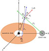Fig. 2. Schematic of interaction between γ-ray photons (generated via synchrotron radiation or inverse Compton scattering) and X-ray photons emitted from the accretion disk or donor star. The path of the X-ray photon from the accretion disk and donor star are marked by the blue line and green line, respectively. The LoS is marked by the red line.

Figure 2 shows the schematic of interaction between γ-ray photons (generated via synchrotron radiation or inverse Compton scattering) and X-ray photons emitted from an accretion disk or donor star. The angle between an X-ray photon emitted from the donor star and the jet is θ′₀, the angle between the LoS and the X-ray photon is θ₀, and the distances from the impact point P to dΩ and the origin O are D_a and D_b, respectively, the angle between $\overline{\mathit{OP}}$ and the z-axis is χ, and the angle between the LoS and the z-axis is θ_i = 27.5° (Miller-Jones et al. 2021).

The interaction between a γ-ray photon and an X-ray photon at the impact point P induces a process γ + γ → e⁺ + e⁻. Then the induced electron e⁻ and positron e⁺ annihilate each other, thus generating photons, neutrinos, mesons, or bosons, depending on the impact conditions (Griffiths 1987).

The γ-ray emission is obtained by solving the radiative transfer equation (Chang & Kiang 2023, 2024)

$$\begin{array}{cc}& \frac{\partial I_{\nu }(\overline{r},\overline{\mathrm{\Omega }})}{\partial s}=j_{\nu }(\overline{r},\overline{\mathrm{\Omega }})-{\kappa }_{\nu }(\overline{r},\overline{\mathrm{\Omega }})I_{\nu }(\overline{r},\overline{\mathrm{\Omega }}),\hfill \end{array}$$(16)

where I_ν is the radiation intensity, j_ν is the emission coefficient, κ_ν is the absorption coefficient, s is the radiation path, and $\overline{\mathrm{\Omega }}$ is the direction of radiation intensity. The radiation is dominated by synchrotron radiation and inverse Compton scattering (de la Cita et al. 2017), with the emission coefficient composed of

$$\begin{array}{cc}& j_{\nu }=j_{\mathrm{sy}}+j_{\mathrm{ic}},\hfill \end{array}$$(17)

where j_sy and j_ic are the spectral emissivities attributed to synchrotron radiation and inverse Compton scattering, respectively.

The plasma in the computational domain is composed of thermal and nonthermal particles. Synchrotron radiation and inverse Compton scattering are contributed by relativistic nonthermal electrons (Dermer & Menon 2009; Rybicki & Lightman 1979), of which the internal energy E′ follows a power-law distribution as (Gomez et al. 1994; Chang & Kiang 2023, 2024)

$$\begin{array}{cc}& \mathrm{d}{n}_e(E\prime )=N\prime (E\prime )\mathrm{d}E\prime =N_0{E}^{\prime -p_e}\mathrm{d}E\prime ,\hfill \end{array}$$(18)

where p_e = 2.2 is the power-law index and N₀ is a normalization factor. We note that the primed variables are defined in the reference frame comoving with the plasma flow. The cooling effect of nonthermal electrons on high-energy emission will be assessed in the next section when describing the simulations of nonthermal emission.

The number density and internal energy density of nonthermal electrons are given by (Chang & Kiang 2024)

$$\begin{array}{cc}\hfill N_e& ={\displaystyle {\int }_{E{\prime }_{min}}^{E{\prime }_{max}}}\mathrm{d}{n}_e(E\prime )\hfill \\ \hfill & =\frac{N_0}{p_e-1}(E_{min}^{\prime -p_e+1}-E_{max}^{\prime -p_e+1})=a_{1}n,\hfill \\ \hfill U_e& ={\displaystyle {\int }_{E{\prime }_{min}}^{E{\prime }_{max}}}E\mathrm{d}{n}_e(E\prime )\hfill \\ \hfill & =\frac{N_0}{p_e-2}(E_{min}^{\prime -p_e+2}-E_{max}^{\prime -p_e+2})=a_2\epsilon ,\hfill \end{array}$$(19)

where E′_min and E′_max are the minimum and maximum internal energies, respectively; n = ρ/m_p is the total electron number density; ε is the total electron internal energy density; and a₁ and a₂ are fractions of nonthermal electron number density and nonthermal internal energy density, respectively, which are determined by fitting the simulated radiation intensity to their observation counterpart, and are set to a₁ = a₂ = 0.03 in this work.

The value of E′_max is estimated from the acceleration timescale of the shock wave, t′_acc = ηE′_max/(q_eB′c) (de la Cita et al. 2016), where q_e is the elementary charge and η = 2π(c/v)². The acceleration timescale is estimated from the synchrotron timescale t′_sync = 1/(a_sB^′2E′_max) and the Bohm diffusion timescale t′_diff = R_a²/(2D′), where a_s = 1.6 × 10⁻³, R_a = 10¹⁰ cm is the typical size of an emitter and D′=cE′_max/(3q_eB′) is the Bohm diffusion coefficient. By setting t′_acc equal to t′_diff and t′_sync, the maximum internal energy is estimated as

$$\begin{array}{cc}& E{\prime }_{max}=min\{\frac{94}{\sqrt{B\prime \eta }},\frac{5.6\times {10}^{-10}B\prime R{\prime }_a}{\sqrt{\eta }}\}.\hfill \end{array}$$(20)

The value of E′_min is determined by taking the ratio of (19) to (20) as

$$\begin{array}{cc}& \frac{U_e}{N_e}=\frac{E_{min}^{\prime -p_e+2}-E_{max}^{\prime -p_e+2}}{E_{min}^{\prime -p_e+1}-E_{max}^{\prime -p_e+1}}\frac{p_e-1}{p_e-2}.\hfill \end{array}$$(21)

The normalization factor N₀ is determined by using (19), given E′_min and E′_max.

The spectral emissivity of synchrotron radiation is given by (Pacholczyk 1970; de la Cita et al. 2016)

$$\begin{array}{c}\hfill j{\prime }_{\mathrm{sy}}(ϵ\prime )=c_{3}B\prime sin\theta \prime {\displaystyle {\int }_{E{\prime }_{min}}^{E{\prime }_{max}}}N\prime (E\prime )F_s(x\prime )\mathrm{d}E\prime ,\end{array}$$(22)

with

$$\begin{array}{c}\hfill F_s(x\prime )={\displaystyle {\int }_{x\prime }^{\infty }}{K}_{5/3}(x)\mathrm{d}x,\end{array}$$(23)

where x′=ϵ′/ϵ′_c, ϵ′_c = c₁hB′ sin θ′E^′2 is the critical energy, c₁ = 3q_e/(4πm_e³c⁵), $c_3=\sqrt{3}{q}_e^3/(4\pi h{m}_e{c}^2)$, K_m(x) is the mth-order modified Bessel function of the second kind, m_e = 9.1 × 10⁻²⁸ g is the electron rest mass, c = 3 × 10¹⁰ cm/s is the speed of light, h is the Planck constant, and θ′ is the angle between B′ and the LoS.

The magnetic field is given by (Rybicki & Lightman 1979)

$$\begin{array}{cc}& \overline{B}{\prime }_{\Vert }={\overline{B}}_{\Vert },\hfill \end{array}$$(24)

$$\begin{array}{cc}& \overline{B}{\prime }_{\perp }=\gamma ({\overline{B}}_{\perp }-\overline{\beta }\times \overline{E}),\hfill \end{array}$$(25)

where $\overline{B}$ and $\overline{E}$ are the magnetic field and electric field, respectively, measured in the observer’s frame.

The spectral emissivity of inverse Compton scattering is given by (Rybicki & Lightman 1979; Chang & Kiang 2024)

$$\begin{array}{cc}& j_{\mathrm{ic}}(ϵ\prime )=\frac{3c{\sigma }_Tϵ\prime }{16\pi }\hfill \\ \hfill & {\displaystyle {\int }_{E{\prime }_{min}}^{E{\prime }_{max}}\int \frac{1}{{\gamma }_e^2ϵ{\prime }_0}}N\prime (E\prime )n{\prime }_0(ϵ{\prime }_0)f(x_{\mathrm{ic}},ϵ{\prime }_0)dϵ{\prime }_{0}dE\prime ,\hfill \end{array}$$(26)

where n′₀(ϵ′₀) is the number density of incident photons at energy ϵ′₀, E′=(γ_e − 1)m_ec², x_ic = ϵ′/(4γ_e²ϵ′₀), σ_T = 8πr_e²/3 is the Thomson cross section, and

$$\begin{array}{c}\hfill f(x_{\mathrm{ic}},{ϵ}_0)=2x_{\mathrm{ic}}ln{x}_{\mathrm{ic}}+x_{\mathrm{ic}}+1-2x_{\mathrm{ic}}^2.\end{array}$$(27)

The number density of incident photons is composed of n′₀(ϵ′₀) = n′_0s(ϵ′₀)+n′_0d(ϵ′₀), where n′_0s(ϵ′₀) accounts for photons from the donor star and n′_0d(ϵ′₀) accounts for photons from the accretion disk. The number density of stellar photons follows a blackbody radiation spectrum (Papavasileiou et al. 2023)

$$\begin{array}{c}\hfill n{\prime }_{0s}(ϵ{\prime }_0)=n_{0s}({ϵ}_0)=\frac{15}{4{\pi }^{5}c}\frac{L_{\mathrm{star}}{\stackrel{\sim }{T}}^4}{{ϵ}_0^2{D}_s^2(e^{\stackrel{\sim }{T}}-1)},\end{array}$$(28)

where D_s is the distance between the donor star and the impact point P; L_star = 3.5 × 10⁵ L_⊙ is the luminosity of the donor star, with L_⊙ = 3.828 × 10³³ erg/s as the solar luminosity; and $\stackrel{\sim }{T}={ϵ}_0/(k_B{T}_{\mathrm{eff}})$, with T_eff = 31 138 K as the effective surface temperature of the donor star (Miller-Jones et al. 2021).

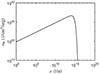Fig. 3. Blackbody radiation spectrum of donor star.

Figure 3 shows the blackbody radiation spectrum of the donor star, where the observed frequency is related to the photon energy as ϵ₀ = hν, with h the Planck constant. The number density of stellar photons is about 4.56 × 10¹⁹ (1/cm³/erg) at ν = 1 Hz, reaches a maximum of n₀ = 1.92 × 10³³ (1/cm³/erg) at ν = 1.01 × 10¹⁴ Hz, and then decreases drastically with frequency. The luminosity of the donor star is

$$\begin{array}{c}\hfill L_{\mathrm{star}}={\displaystyle \int 4\pi }{D}_s^{2}c{n}_0({ϵ}_0){ϵ}_{0}d{ϵ}_0=1.34\times {10}^{39}(\mathrm{erg}/\mathrm{s}).\end{array}$$(29)

The number density of disk photons is the integration of a blackbody spectrum over the accretion disk as (Cerutti et al. 2011; Papavasileiou et al. 2023)

$$\begin{array}{cc}& n{\prime }_{0d}(ϵ{\prime }_0)=n_{0d}({ϵ}_0)={\displaystyle \int \frac{2}{h^3{c}^3}}\frac{{ϵ}_0^2}{[e^{{ϵ}_0/(k_{B}T)}-1]}\mathrm{d}\mathrm{\Omega }\hfill \\ \hfill & ={\displaystyle {\int }_0^{2\pi }}{\displaystyle {\int }_{r_{\mathrm{in}}}^{r_{\mathrm{out}}}}\frac{2}{h^3{c}^3}\frac{{ϵ}_0^2}{[e^{{ϵ}_0/(k_{B}T)}-1]}\frac{D_b·cos\chi }{D_a^3}r\mathrm{d}r\mathrm{d}\varphi ,\hfill \end{array}$$(30)

where r_out = 10¹² cm; r_in = 6r_g (Salvo et al. 2001), with r_g = GM_BH/c² the gravitational radius of the black hole; and M_BH = 21.2 M_⊙, with M_⊙ as the solar mass (Miller-Jones et al. 2021).

It should be noted that the computational domain does not include the vicinity of the black hole at the length scale of several r_g, but the contribution of the X-ray emitting accretion disk, which can extend to about 6r_g, is included in the simulations (Salvo et al. 2001).

The temperature distribution of the accretion disk is specified as (Papavasileiou et al. 2023)

$$\begin{array}{c}\hfill T(r)=T_g{\left[\frac{r\prime -2/3}{r\prime {(r\prime -2)}^3}(1-\frac{3\sqrt{3}(r\prime -2)}{\sqrt{2}r\prime \sqrt{r\prime }})\right]}^{1/4},\end{array}$$(31)

where

$$\begin{array}{c}\hfill T_g={\left(\frac{3G{M}_{\mathrm{BH}}{\dot{M}}_{\mathrm{accr}}}{8\pi {\sigma }_{\mathrm{SB}}{r}_g^3}\right)}^{1/4}\end{array}$$(32)

is the highest temperature closest to the black hole, r′=r/r_g, σ_SB is the Stefan-Boltzmann constant, and Ṁ_accr = 10⁻⁸ M_⊙/yr is the accretion rate of the system.

The photon energy and the emission energy spectrum in the plasma comoving frame are related to their counterparts in the observer’s frame as (Rybicki & Lightman 1979; Chang & Kiang 2023)

$$\begin{array}{cc}\hfill ϵ& =\delta ϵ\prime ,\hfill \\ \hfill ϵj_{\nu }(ϵ)& ={\delta }^4ϵ\prime j{\prime }_{\nu }(ϵ\prime ),\hfill \end{array}$$(33)

where δ = [γ(1 − β cos θ_obs)]⁻¹ is the Doppler factor, γ is the Lorentz factor, and θ_obs is the angle between the jet and the observation direction, with θ_obs ≃ θ_i, as shown in Fig. 2.

2.3. Absorption attributed to accretion disk and donor star

The γ-ray emission via synchrotron radiation and inverse Compton scattering, as described in Section 2.2, is partially absorbed by the emission from the accretion disk and the donor star, while the absorption by the emission from the black hole corona is negligible (Papavasileiou et al. 2023). Thus, the absorption coefficient can be approximated as

$$\begin{array}{cc}& {\kappa }_{\nu }={\kappa }_{\nu \mathrm{disk}}+{\kappa }_{\nu \mathrm{star}}(1/\mathrm{cm}),\hfill \end{array}$$(34)

where κ_νdisk and κ_νstar are the absorption coefficients attributed to the accretion disk and the donor star, respectively.

The differential absorption coefficient attributed to X-ray emission from the accretion disk in energy interval dϵ_d and directional interval dΩ = (D_b cos χ/D_a³)rdrdϕ is given by (Becker & Kafatos 1995; Cerutti et al. 2011; Papavasileiou et al. 2023)

$$\begin{array}{cc}& \mathrm{d}{\kappa }_{\nu \mathrm{disk}}=\frac{2}{h^3{c}^3}\frac{{ϵ}_d^2}{[e^{{ϵ}_d/(k_{B}T)}-1]}\hfill \\ \hfill & (1-cos{\theta }_0){\sigma }_{\gamma \gamma }\mathrm{d}\mathrm{\Omega }\mathrm{d}{ϵ}_d,\hfill \end{array}$$(35)

where

$$\begin{array}{cc}& {\sigma }_{\gamma \gamma }=\frac{3}{16}{\sigma }_T(1-{\beta }^2)\hfill \\ \hfill & [(3-{\beta }^4)ln\left(\frac{1+\beta }{1-\beta }\right)-2\beta (2-{\beta }^2)]\hfill \end{array}$$(36)

is the pair-production cross section of the process γ + γ → e⁺ + e⁻ with Γ² = 1/(1 − β²) = ϵ_dϵ_γ(1 − cos θ_γγ)/(2m_e²c⁴), β is the velocity of positron or electron in units of c, σ_T is the Thomson cross section of a positron or electron, ϵ_d is the energy of X-ray photon, ϵ_γ is the energy of γ-ray photon, θ_γγ is the angle between the X-ray photon and the γ-ray photon, h is the Planck constant, and k_B is the Boltzmann constant. We note that the first subscript of σ_γγ indicates a γ-ray photon generated via synchrotron radiation or inverse Compton scattering, and the second subscript indicates an X-ray photon emitted from the accretion disk or the donor star.

The absorption coefficient attributed to the accretion disk can thus be derived by integrating (33) as

$$\begin{array}{cc}& {\kappa }_{\nu \mathrm{disk}}=\frac{2}{h^3{c}^3}{\displaystyle {\int }_{{ϵ}_{min}}^{\infty }}{\displaystyle {\int }_0^{2\pi }}{\displaystyle {\int }_{r_{\mathrm{in}}}^{r_{\mathrm{out}}}}\frac{{ϵ}_d^2}{[e^{{ϵ}_d/(k_{B}T)}-1]}\hfill \\ \hfill & \times (1-cos{\theta }_0){\sigma }_{\gamma \gamma }\frac{D_b·cos\chi }{D_a^3}rdrd\varphi d{ϵ}_d,\hfill \end{array}$$(37)

where ϵ_min = 2m_e²c⁴/[ϵ_γ(1 − cos θ₀)], m_e is the electron rest-mass, r_out = 10¹² cm, r_in = 6r_g, r_g = GM_BH/c² is the gravitational radius of the black hole, and M_BH = 21.2 M_⊙, with M_⊙ as the solar mass.

Similarly, the absorption coefficient attributed to the donor star is given by (Papavasileiou et al. 2023; Böttcher & Dermer 2005)

$$\begin{array}{c}\hfill {\kappa }_{\nu \mathrm{star}}={\displaystyle {\int }_{{ϵ}_{min}}^{\infty }}\frac{d{n}_{\mathrm{ph}}}{\mathrm{d}ϵ}{\sigma }_{\gamma \gamma }(1-cos{\theta }_0)\mathrm{d}ϵ,\end{array}$$(38)

where dn_ph/dϵ = n₀(ϵ₀) is the photon number density of blackbody radiation from the donor star.

3. Simulations and discussions

3.1. Interaction between jet and stellar wind

The average gas pressure is related to the temperature T via the ideal gas law as (Chang & Kiang 2023)

$$\begin{array}{c}\hfill ⟨p_j⟩=\frac{\rho }{N_0\mu m_p}RT\end{array}$$(39)

where N₀ = 6.02 × 10²³ is Avogadro’s number, m_p is the proton mass, R = 8.314 × 10⁷ (erg/mol/K), and μ is the average particle weight, with μ = 0.5 if protons dominate.

The temperature and magnetic field profile of the jet in Cygnus X-1 are not well known (Perucho et al. 2010; López-Miralles et al. 2022). In Perucho et al. (2010), a hydrodynamic jet with a temperature of 10¹⁰ K was simulated. A forward shock was formed as the jet roared through the stellar wind, and recollimation shocks were forged by the initial overpressure in the jet. In López-Miralles et al. (2022), the simulated features of weakly magnetized jets with T ≃ 1.7 × 10⁹ K resembled those of hydrodynamic jets in Perucho et al. (2010). The strongly magnetized jet with T ≃ 1.4 × 10¹² K manifested current-driven instabilities and more recollimation shocks within the jet. In Tetarenko et al. (2019), the brightness temperature of the jet in Cygnus X-1 was estimated as T_b ≃ 10⁹ K at a frequency of 11 GHz, but the weights of the contributions from thermal and nonthermal emissions remained elusive. For this work, the jet temperature of T = 10⁹ K was adopted in the simulations.

We assumed that the jet is composed of protons and electrons with the same number density and the mass density of the jet is ρ_j = 2.8 × 10⁻¹⁵ g/cm³. The average gas pressure was estimated as ⟨p_j⟩ = 463 erg/cm³ by using Eq. (37). The Lorentz factor of the jet was estimated as γ = 2.59 (Tetarenko et al. 2019), with an eruption speed of v_j = 0.92.

The magnetization β_j and the magnetic pitch angle ϕ_j of the jet are defined as (Chang & Kiang 2023)

$$\begin{array}{cc}& {\beta }_j=\frac{⟨b_j^2⟩}{2⟨p_j⟩},\hfill \end{array}$$(40)

$$\begin{array}{cc}& {\varphi }_j={tan}^{-1}\frac{⟨B_{\varphi }⟩}{B_{z0}},\hfill \end{array}$$(41)

where

$$\begin{array}{cc}& ⟨b_j^2⟩=\frac{{⟨B_{\varphi }⟩}^2}{{\gamma }^2}+B_{z0}^2,\hfill \end{array}$$(42)

$$\begin{array}{cc}& ⟨B_{\varphi }⟩=\frac{{\displaystyle {\int }_0^1}{B}_{\varphi }(r)r\mathrm{d}r}{{\displaystyle {\int }_0^1}r\mathrm{d}r}\hfill \\ \hfill & =4B_{\varphi 0}{R}_{\varphi 0}(1-R_{\varphi 0}{tan}^{-1}\frac{1}{R_{\varphi 0}}).\hfill \end{array}$$(43)

In López-Miralles et al. (2022), toroidal magnetic fields with β = 1.03 and 1.56, respectively, were assumed to simulate jet–wind interactions in HMXRBs. The magnetic field can stabilize the jet evolution if the magnetic energy flux is lower than the kinetic energy flux. A strong magnetic energy flux tends to destabilize the plasma flow, ensuing more energy dissipation and slower velocity in the jet head. In this work, the relativistic jet is assumed to burst in a toroidal magnetic field (ϕ_j = 90°), with β_j = 1.

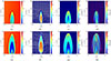Fig. 4. Interaction between a relativistic magnetized jet and a stellar wind: (a) ρ at t = 25 s, (b) γ at t = 25 s, (c) p at t = 25 s, (d) $|\overline{B}|$ at t = 25 s, (e) ρ at t = 50 s, (f) γ at t = 50 s, (g) p at t = 50 s, (h) $|\overline{B}|$ at t = 50 s. The streamlines in (b) and (f) indicate plasma flow, the streamlines in (d) and (h) indicate magnetic field lines.

Figure 4 shows the interaction between a relativistic magnetized jet and a stellar wind. The snapshots of plasma variables at t = 25 and 50 s, respectively, are presented to manifest the evolution of the jet–wind interaction. Figures 4(a)–4(d) show that at t = 25 s the jet manifests a spine-sheath with ρ ≃ 2 × 10⁻¹⁵ g/cm³ in the central spine region and dilutes away from it. A shock front is forged by the relativistic jet and reaches z ≃ 67.2R_j (4.03 × 10¹¹ cm), carrying mass density of ρ ≃ 10⁻¹⁴ g/cm³ and gas pressure of p ≃ 10⁵ erg/cm³. The shock front is followed by a rarefied sheath region with lower mass density and gas pressure. The Lorentz factor in the central spine region of the jet is γ ≃ 2.5. The magnetic field manifests a petal-like shape with $|\overline{B}|\simeq {10}^2$-10³ gauss in the jet region. The stellar wind blows into the computational domain from the donor star, with v_w = 2 × 10⁸ cm/s, leading to a fanning-out pattern of plasma flow and slightly skewed patterns of ρ, p, and $|\overline{B}|$ about the z-axis.

Figures 4(e)–4(h) show that at t = 50 s, the jet reaches z ≃ 110.2R_j (6.61 × 10¹¹ cm), and is blown by the stellar wind to incline toward the −y direction. A forward shock and a cocoon-like region (enclosed by a white contour) are formed, and a spine-sheath region (enclosed by a red contour) is formed within the cocoon. The gas pressure within the cocoon drops suddenly across the red contour. The gas pressure around the nose cone (marked by a red arrow) is higher than that within the cocoon as the shock front pushes forward, similar to the observed features in Leismann et al. (2005). The mass density in the cocoon region is ρ ≃ 10⁻¹⁶–10⁻¹⁵ g/cm³, and that within the red contour decreases to ρ ≃ 10⁻¹⁷ g/cm³, except near the origin of the jet. The Lorentz factor between the red and white contours is γ ≃ 1.5, and that within the red contour increases to γ ≃ 2.1. The gas pressure between the red and white contours is higher than 10⁴ erg/cm³, and that within the red contour drops to 10² erg/cm³, except near the origin of the jet. The mass density and gas pressure increase near the black hole. The magnetic field manifests a petal-like shape with $|\overline{B}|\simeq {10}^2$–10³ gauss in the jet region. The magnetic field strength increases to $|\overline{B}|\simeq {10}^4$ gauss near the black hole.

The jet eruption halts at t = 50 s. The previous jet burst moves out of the computational domain, forming a depletion region in which the magnitudes of mass density, Lorentz factor, internal energy, and magnetic field are lower than its surrounding.

In short, the evolution of a jet eruption through a background stellar wind over a region of 10¹² cm in scale was simulated; it manifested many detailed features with a spatial resolution of 1.5 × 10⁹ cm. It provides useful clues for future observations, in which the current resolution in detecting γ-ray photons is about 5′ (≃10¹⁹ cm) (Sabatini et al. 2013; Zanin et al. 2016).

3.2. Nonthermal emission

The γ-ray emission from Cygnus X-1 was estimated to originate from a region farther than 10¹¹ cm from and nearer than 10¹³ cm to the black hole (Zanin et al. 2016). The nonthermal emission model in Section 2.2 can be used to reconstruct the γ-ray emission in terms of the plasma distributions simulated with the RMHD model.

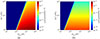Fig. 5. Spectral emissivity (a) jsy attributed to synchrotron radiation and (b) jic attributed to inverse Compton scattering, N0 = 1, $|\overline{B}|=1000$ (G), θ′=π/2, (x, y, z) = (0, 0, 1012) cm.

Figure 5 shows the spectral emissivity j_sy attributed to synchrotron radiation and inverse Compton scattering in Eq. (23) and Eq. (26), respectively. Figure 5(a) shows the spectral emissivity j_sy attributed to synchrotron radiation, as a function of photon energy ϵ′=hν′ and maximum internal energy E′_max of nonthermal electrons. At a given photon energy level, the emissivity rises suddenly from 0 to a plateau when E′_max is increased across certain threshold. The typical value of E′_max estimated with (21) is about 10¹¹–10¹² eV; the pumping synchrotron radiation energy is about ϵ′ = 10⁹–10¹⁰ eV. Figure 5(b) shows the spectral emissivity attributed to inverse Compton scattering in terms of ϵ′ and E′_max. A similar threshold of E′_max is observed. With E′_max ≃ 10¹¹–10¹² eV, the emission energy attributed to inverse Compton scattering is about ϵ′ = 10¹² eV. A comparison of Figures 5(a) and 5(b), shows that the E′_max threshold of inverse Compton scattering is lower than that of synchrotron radiation, and the magnitude of synchrotron radiation is larger than that of inverse Compton scattering.

The typical value of E′_max is several hundred GeV in the jet region. The synchrotron radiation with a higher photon energy ϵ′=hν′ requires a higher E′_max threshold, and hence the synchrotron radiation prevails at lower photon energies. On the same argument, the emission at higher energies is dominated by the inverse Compton scattering.

The cooling effect on nonthermal electrons is exerted by the Coulomb interaction of low-energy electrons, as well as synchrotron radiation and inverse Compton scattering of high-energy electrons, characterized with the cooling timescales (Miniati 2001; Chang & Kiang 2024)

$$\begin{array}{cc}& {\tau }_{\mathrm{Comb}}=2.53\times {10}^9\left(\frac{|\overline{p}|}{100m_{e}c}\right){\left(\frac{n}{{10}^{-3}}\right)}^{-1}(\mathrm{yr}),\hfill \\ \hfill & {\tau }_{\mathrm{sync}+\mathrm{IC}}=2.3\times {10}^8{\left(\frac{|\overline{p}|}{{10}^4{m}_{e}c}\right)}^{-1}{(1+\frac{u_B}{u_{\mathrm{cmb}}})}^{-1}(\mathrm{yr}),\hfill \end{array}$$(44)

respectively, where $|\overline{p}|$ is the electron momentum, n is the electron number density, $u_B={|\overline{B}|}^2/(8\pi )$ and u_cmb = 4.2 × 10⁻¹³ erg/cm³ are the energy densities of the magnetic field and cosmic microwave background, respectively. Their values in the simulations on Cygnus X-1 are n = 10⁻¹⁶ cm⁻³, $|\overline{B}|=1000$ gauss, τ_Comb ≃ 10¹⁰ yr and τ_{sync + IC} ≃ 10⁵ yr at E′ = 1 MeV, and τ_Comb ≃ 10¹⁵ yr and τ_{sync + IC} ≃ 3.7 yr at E′ = 100 GeV. Since the cooling timescales are much longer than the dynamical timescale of Cygnus X-1, the cooling effect is negligible in computing the nonthermal emissions.

To obtain spectral energy distributions that are comparable to the observations, radiation maps at different photon energies and a specific azimuth angle ϕ_i are computed first by integrating (16) along the line of sight. Then, these radiation maps are integrated over a solid angle extended by Cygnus X-1. The emissivity and absorption coefficients in (16) are computed by using (23), (26), (34), and (36), respectively, with the plasma distribution shown in Fig. 4, at t = 50 s. The radiation maps at the simulated resolution cannot be observed directly, but they can provide clues to understanding the nonthermal emission distribution.

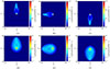Fig. 6. Radiation intensity Iν with photon energy ϵ from Cygnus X-1 observed at different azimuth angles, (a) ϵ = 1 MeV, ϕi = −π/2, (b) ϵ = 1 MeV, ϕi = 0, (c) ϵ = 1 MeV, ϕi = π/2, (d) ϵ = 1 GeV, ϕi = −π/2, (e) ϵ = 1 GeV, ϕi = 0, (f) ϵ = 1 GeV, ϕi = π/2.

Figure 6 shows the radiation intensity I_ν (erg/s/sr/eV/cm²) from Cygnus X-1, at specific frequency ν, which is obtained by solving the radiative transfer equation in Eq. (16) and then projected onto the plane of the sky, as shown in Fig. 1. The azimuth angle ϕ_i is arbitrarily set to −π/2, 0, and π/2, respectively, to demonstrate the flux orbital variability. Cygnus X-1 is observed from the upwind direction if ϕ_i = π/2, and from the downwind direction if ϕ_i = −π/2. The emissions concentrate around the origin. Subtle differences appear in the internal structure at a resolution much finer than that of observation. The differences are attributed to the asymmetrical emission and absorption aroused by the stellar wind, thus resulting in flux orbital variability.

Figure 6(a) shows that at ϵ = hν = 1 MeV, the jet observed at ϕ_i = −π/2 travels in the y′ direction. The emission around the origin is about I_ν = 10¹⁰ erg/s/sr/eV/cm², and drops to about I_ν = 10⁶ erg/s/sr/eV/cm² in the jet head. The emission at ϵ = 1 MeV is dominated by synchrotron radiation. The emission pattern is highly affected by the magnetic field strength, which is relatively high around the origin and the jet head.

The per-unit-energy radiation flux at specific ϵ is computed by integrating I_ν(ϵ) over a solid angle Ω extended by Cygnus X-1 as

$$\begin{array}{c}\hfill F(ϵ)=ϵN_{\mathrm{ph}}(ϵ)={\displaystyle {\int }_{\mathrm{\Omega }}}{I}_{\nu }(ϵ)\mathrm{d}\mathrm{\Omega },\end{array}$$(45)

where N_ph(ϵ) is the photon number density in unit of counts/s/eV/cm². The corresponding radiation flux in Fig. 6(a) is ϵF(ϵ) = 3.66 × 10⁻⁹ erg/s/cm².

Figures 6(b) and 6(c) show that the jet observed at ϕ_i = 0 and π/2 traverses in the −x′ direction and −y′ direction, respectively. These two emission patterns appear similar. The radiation flux at ϕ_i = 0 is ϵF(ν) = 5.05 × 10⁻⁹ erg/s/cm², and that at ϕ_i = π/2 is ϵF(ν) = 4.10 × 10⁻⁹ erg/s/cm². The difference in radiation fluxes at different ϕ_i values verifies the flux orbital variability.

Figure 6(d) shows that at ϵ = hν = 1 GeV the jet observed at ϕ_i = −π/2 traverses in the y′ direction. The emission around the origin drops to I_ν = 10³ erg/s/sr/eV/cm², and that in the jet it is about I_ν = 10⁻¹ erg/s/sr/eV/cm². Nonthermal electrons permeate the whole jet, and inverse Compton scattering prevails in high-energy emission, and thus the emission is contributed by the whole jet. The radiation flux is ϵF(ν) = 1.40 × 10⁻¹² erg/s/cm². Figures 6(e) and 6(f) show similar features to those in Fig. 6(d), while their traversing directions are different. The radiation flux at ϕ_i = 0 is ϵF(ν) = 1.73 × 10⁻¹² erg/s/cm², and that at ϕ_i = π/2 is ϵF(ν) = 1.51 × 10⁻¹² erg/s/cm². The phenomenon of flux orbital variability is verified again.

The current resolution of γ-ray photon detection is about 5′ (≃10¹⁹ cm), and hence detailed features of emission cannot be revealed on the plane of the sky (Sabatini et al. 2013; Zanin et al. 2016). In this work, the distribution of emission from a jet eruption through the background stellar wind is computed on the length scale of about 10¹² cm, with resolution of 1.5 × 10⁹ cm, which can provide useful clues to the detailed features for future studies.

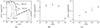Fig. 7. Spectra of radiation flux from Cygnus X-1. Panel (a) Spectrum in 104 ≤ ϵ ≤ 1014 eV; panel (b) spectrum in 104 ≤ ϵ ≤ 108 eV; panel (c) spectrum in 109 ≤ ϵ ≤ 1013 eV. The color-coding is as follows: •ϕi = −π/2, •ϕi = 0, •ϕi = π/2. The black curves are computed with the typical jet parameters: ρ = 2.8 × 10−15 g/cm3, p = 106 erg/cm3, and $|\overline{B}|={10}^3$ gauss, under different E′max.

Figure 7 shows the spectra of radiation flux ϵF(ν) computed with photon energies in the range 10 keV≤ϵ ≤ 100 TeV, and ϕ_i = −π/2, 0, and π/2, respectively, where F(ν) is the per-unit-energy radiation flux computed with (42). We assume that the photon number density follows a power-law distribution, N_ph(ϵ)∝ϵ^−Γ, where Γ is the photon index. In Zanin et al. (2016), the photon index of Cygnus X-1 was estimated as Γ = 2.3 ± 0.2, leading to F ∝ ϵ^−α and ϵF ∝ ϵ^−α′, with α = Γ − 1 and α′=Γ − 2. In Zanin et al. (2016), the photon index of Cygnus X-1 was estimated from the observed spectrum as Γ = 2.3 ± 0.2.

Figure 7(a) shows the spectra of radiation flux computed with different photon energies and different azimuth angles. By regressing upon the simulation data, the power-law indices at ϕ_i = −π/2, 0 and ϕ_i = π/2 are α′ = 0.38, 0.34 and 0.36, respectively, corresponding to the photon indices of Γ = 2.38, 2.34 and 2.36, respectively. For ϵ ≤ 10⁶ eV, the radiation flux ϵF at ϕ_i = −π/2 is the highest and that at ϕ_i = 0 is the lowest. For ϵ ≥ 10⁹ eV, the radiation flux at ϕ_i = 0 is the highest and that at ϕ_i = −π/2 is the lowest.

The black curves represent the estimated radiation flux computed with typical jet parameters, ρ = 2.8 × 10⁻¹⁵ g/cm³, p = 10⁶ erg/cm³, and $|\overline{B}|={10}^3$ gauss, under different E′_max. The radiation flux is estimated as ϵF = ϵj_νV/(4πd²), where j_ν is the emissivity computed with typical jet parameters, V is the jet volume, and d = 2.22 kpc is the distance between Cygnus X-1 and the Earth (Zanin et al. 2016; Miller-Jones et al. 2021). The emission mainly comes from the vicinity of the origin, with the volume approximated as a cylinder with radius 5R_j and height 20R_j, leading to V ≃ 10³²π cm³. The emission in ϵ ≃ 10⁴–10⁷ eV is mainly attributed to synchrotron radiation, and that in ϵ ≃ 10⁹–10¹⁴ eV is mainly attributed to inverse Compton scattering. The simulated data fit the curve with E′_max = 600 GeV well.

It is observed that for ϵ ≤ 10⁸ eV, the fluxes observed at ϕ_i = ±π/2 are stronger than that at ϕ_i = 0. For ϵ ≥ 10⁹ eV, the fluxes observed at ϕ_i = ±π/2 are weaker than that at ϕ_i = 0.

Figure 7(b) shows the spectrum in 10⁴ ≤ ϵ ≤ 10⁸ eV. The radiation fluxes observed in the upwind and downwind directions are stronger than that at ϕ_i = 0. In general, the fluxes observed in the downwind direction (ϕ_i = −π/2) are stronger than those in the upwind direction (ϕ_i = π/2), except at ϵ = 10⁷ eV.

Figure 7(c) shows the spectrum in 10⁹ ≤ ϵ ≤ 10¹³ eV. The radiation fluxes observed in the upwind and downwind directions are weaker than that at ϕ_i = 0. The fluxes observed in the downwind direction (ϕ_i = −π/2) are weaker than those in the upwind direction (ϕ_i = π/2).

4. Conclusions

The plasma evolution and high-energy emission from a relativistic magnetized jet traversing a stellar wind were simulated and analyzed. A self-consistent RMHD model was applied, which takes into account the interaction among the relativistic jet, stellar wind, and magnetic field. The relevant parameters were estimated from the data of Cygnus X-1 in Fermi observation, and hence the simulated spectrum closely matches the observed counterpart. The fine features of high-energy emissions, not available in the observation, were acquired as useful clues for future studies. The simulated jet dynamics, radiation map, flux orbital variability, spectrum of radiation flux, and photon index were justified with consistent models, and validated wherever possible with available observation data. The observed spectral features between 10⁴–10¹³ eV and the flux orbital variability were reproduced, and their radiation mechanisms were analyzed by simulations.

We found that a jet drives a shock front, which is followed by a rarefied region of lower mass density and gas pressure. The distributions of mass density, plasma flow speed, pressure, and magnetic field manifest petal-like shapes around the jet region. The emission at lower energy is mainly contributed by synchrotron radiation, and that at higher energy it is mainly contributed by inverse Compton scattering. The emissivity is negligible if the maximum electron internal energy E′_max falls below a certain threshold, and significantly increases if E′_max rises above the threshold.

The emission pattern of radiation intensity I_ν, induced by the jet–wind interaction on the plane of the sky at various photon energies are computed. Separate spectra contributed by synchrotron radiation and inverse Compton scattering are also derived. The radiation flux at different azimuth angles ϕ_i manifests the orbital variability. The photon indices regressed from the simulation data are Γ = 2.38, 2.34, and 2.36 at ϕ_i = −π/2, 0, and π/2, respectively.

Acknowledgments

This work was partly sponsored by the National Science and Technology Council, Taiwan, under Project NSTC 113-2221-E-002-150-MY2.

References

All Figures

	Fig. 1. Schematic of a relativistic magnetized jet erupting from a HMMQ.
In the text

	Fig. 2. Schematic of interaction between γ-ray photons (generated via synchrotron radiation or inverse Compton scattering) and X-ray photons emitted from the accretion disk or donor star. The path of the X-ray photon from the accretion disk and donor star are marked by the blue line and green line, respectively. The LoS is marked by the red line.
In the text

	Fig. 3. Blackbody radiation spectrum of donor star.
In the text

	Fig. 4. Interaction between a relativistic magnetized jet and a stellar wind: (a) ρ at t = 25 s, (b) γ at t = 25 s, (c) p at t = 25 s, (d) $|\overline{B}|$ at t = 25 s, (e) ρ at t = 50 s, (f) γ at t = 50 s, (g) p at t = 50 s, (h) $|\overline{B}|$ at t = 50 s. The streamlines in (b) and (f) indicate plasma flow, the streamlines in (d) and (h) indicate magnetic field lines.
In the text

	Fig. 5. Spectral emissivity (a) jsy attributed to synchrotron radiation and (b) jic attributed to inverse Compton scattering, N0 = 1, $|\overline{B}|=1000$ (G), θ′=π/2, (x, y, z) = (0, 0, 1012) cm.
In the text

	Fig. 6. Radiation intensity Iν with photon energy ϵ from Cygnus X-1 observed at different azimuth angles, (a) ϵ = 1 MeV, ϕi = −π/2, (b) ϵ = 1 MeV, ϕi = 0, (c) ϵ = 1 MeV, ϕi = π/2, (d) ϵ = 1 GeV, ϕi = −π/2, (e) ϵ = 1 GeV, ϕi = 0, (f) ϵ = 1 GeV, ϕi = π/2.
In the text

	Fig. 7. Spectra of radiation flux from Cygnus X-1. Panel (a) Spectrum in 104 ≤ ϵ ≤ 1014 eV; panel (b) spectrum in 104 ≤ ϵ ≤ 108 eV; panel (c) spectrum in 109 ≤ ϵ ≤ 1013 eV. The color-coding is as follows: •ϕi = −π/2, •ϕi = 0, •ϕi = π/2. The black curves are computed with the typical jet parameters: ρ = 2.8 × 10−15 g/cm3, p = 106 erg/cm3, and $|\overline{B}|={10}^3$ gauss, under different E′max.
In the text

References

- Akharonian, F. A., & Vardanian, V. V. 1985, Ap&SS, 115, 31 [Google Scholar]
- Albert, J., Aliu, E., Anderhub, H., et al. 2007, ApJ, 665, L51 [NASA ADS] [CrossRef] [Google Scholar]
- Becker, P. A., & Kafatos, M. 1995, ApJ, 453, 83 [Google Scholar]
- Böttcher, M., & Dermer, C. D. 2005, ApJ, 634, L81 [CrossRef] [Google Scholar]
- Cerutti, B., Dubus, G., Malzac, J., et al. 2011, A&A, 529, A120 [NASA ADS] [CrossRef] [EDP Sciences] [Google Scholar]
- Chang, C.-J., & Kiang, J.-F. 2023, Universe, 9(5), 235 [Google Scholar]
- Chang, C.-J., & Kiang, J.-F. 2024, Universe, 10(7), 279 [Google Scholar]
- de la Cita, V. M., Bosch-Ramon, V., Paredes-Fortuny, X., Khangulyan, D., & Perucho, M. 2016, A&A, 591, A15 [NASA ADS] [CrossRef] [EDP Sciences] [Google Scholar]
- de la Cita, V. M., del Palacio, S., Bosch-Ramon, V., et al. 2017, A&A, 604, A39 [NASA ADS] [CrossRef] [EDP Sciences] [Google Scholar]
- Dermer, C. D., & Menon, G. 2009, High Energy Radiation from Black Holes: Gamma Rays, Cosmic Rays, and Neutrinos [Google Scholar]
- El Mellah, I., Sundqvist, J. O., & Keppens, R. 2017, MNRAS, 475, 3240 [Google Scholar]
- Gallo, E., Miller, B. P., & Fender, R. 2012, MNRAS, 423, 590 [Google Scholar]
- Gomez, J. L., Alberdi, A., & Marcaide, J. M. 1994, A&A, 284, 51 [NASA ADS] [Google Scholar]
- Griffiths, D. 1987, Introduction to Elementary Particles (Wiley-VCH) [Google Scholar]
- Leismann, T., Antón, L., Aloy, M. A., et al. 2005, A&A, 436, 503 [NASA ADS] [CrossRef] [EDP Sciences] [Google Scholar]
- Londrillo, P., & Del Zanna, L. 2004, J. Comput. Phys., 195, 17 [NASA ADS] [CrossRef] [Google Scholar]
- López-Miralles, J., Perucho, M., Martí, J. M., Migliari, S., & Bosch-Ramon, V. 2022, A&A, 661, A117 [NASA ADS] [CrossRef] [EDP Sciences] [Google Scholar]
- Malyshev, D., Zdziarski, A. A., & Chernyakova, M. 2013, MNRAS, 434, 2380 [NASA ADS] [CrossRef] [Google Scholar]
- Markoff, S., Nowak, M., Corbel, S., Fender, R., & Falcke, H. 2003, A&A, 397, 645 [CrossRef] [EDP Sciences] [Google Scholar]
- Mignone, A., & Bodo, G. 2006, MNRAS, 368, 1040 [Google Scholar]
- Miller-Jones, J. C. A., Bahramian, A., Orosz, J. A., et al. 2021, Science, 371, 1046 [Google Scholar]
- Miniati, F. 2001, CPC, 141, 17 [NASA ADS] [Google Scholar]
- Pacholczyk, A. G. 1970, Radio astrophysics. Nonthermal processes in galactic and extragalactic sources [Google Scholar]
- Papavasileiou, T. V., Kosmas, O. T., & Sinatkas, I. 2023, A&A, 673, A162 [NASA ADS] [CrossRef] [EDP Sciences] [Google Scholar]
- Perucho, M., & Bosch-Ramon, V. 2008, A&A, 482, 917 [NASA ADS] [CrossRef] [EDP Sciences] [Google Scholar]
- Perucho, M., Bosch-Ramon, V., & Khangulyan, D. 2010, A&A, 512, L4 [NASA ADS] [CrossRef] [EDP Sciences] [Google Scholar]
- Reid, M. J., McClintock, J. E., Narayan, R., et al. 2011, ApJ, 742, 83 [Google Scholar]
- Rodriguez, J., Grinberg, V., Laurent, P., et al. 2015, Spectral state dependence of the 0.4-2 MeV polarized emission in Cygnus X-1 seen with INTEGRAL/IBIS, and links with the AMI radio data [Google Scholar]
- Rybicki, G. B., & Lightman, A. P. 1979, Radiative processes in astrophysics [Google Scholar]
- Sabatini, S., Tavani, M., Coppi, P., et al. 2013, ApJ, 766, 83 [Google Scholar]
- Salvo, T. D., Done, C., Zycki, P. T., Burderi, L., & Robba, N. R. 2001, ApJ, 547, 1024 [NASA ADS] [CrossRef] [Google Scholar]
- Shapiro, S. L., Lightman, A. P., & Eardley, D. M. 1976, ApJ, 204, 187 [NASA ADS] [CrossRef] [Google Scholar]
- Sundqvist, J. O., Owocki, S. P., & Puls, J. 2018, A&A, 611, A17 [NASA ADS] [CrossRef] [EDP Sciences] [Google Scholar]
- Tetarenko, A. J., Casella, P., Miller-Jones, J. C. A., et al. 2019, MNRAS, 484, 2987 [NASA ADS] [CrossRef] [Google Scholar]
- Toro, E. F. 2009, Riemann Solvers and Numerical Methods for FluidDynamics: A Practical Introduction [Google Scholar]
- Zanin, R., Fernández-Barral, A., de Oña Wilhelmi, E., et al. 2016, A&A, 596, A55 [NASA ADS] [CrossRef] [EDP Sciences] [Google Scholar]
- Zdziarski, A. A., & Gierliński, M. 2004, PTP Supplement, 155, 99 [Google Scholar]