| Issue |
A&A
Volume 705, January 2026
|
|
|---|---|---|
| Article Number | A140 | |
| Number of page(s) | 8 | |
| Section | Astrophysical processes | |
| DOI | https://doi.org/10.1051/0004-6361/202554175 | |
| Published online | 14 January 2026 | |
The 3D pulsar magnetosphere with machine learning: First results
1
Department of Physics, University of Patras Rio 26504, Greece
2
Research Center for Astronomy and Applied Mathematics, Academy of Athens Athens 11527, Greece
3
Department of Electrical Engineering, National Technical University of Athens Athens 15772, Greece
★ Corresponding authors: This email address is being protected from spambots. You need JavaScript enabled to view it.
, This email address is being protected from spambots. You need JavaScript enabled to view it.
Received:
18
February
2025
Accepted:
16
November
2025
Abstract
Context. All particle-in-cell (PIC) simulations of the pulsar magnetosphere over the past decade show closed line regions that end a significant distance inside the light cylinder, and manifest thick, strongly dissipative separatrix surfaces instead of thin current sheets, with a tip that has a distinct pointed Y shape rather than a T shape.
Aims. We need to understand the origin of these results, which were not predicted by our earlier numerical simulations of the pulsar magnetosphere. To gain new insight into this problem, we set out to obtain the theoretical steady-state solution of the ideal 3D force-free magnetosphere with zero dissipation along the separatrix and equatorial current sheets. To achieve this goal, we developed a novel numerical method.
Methods. We solved two independent magnetospheric problems without current sheet discontinuities in the domains of open and closed field lines and adjusted the shape of their interface (the separatrix) to satisfy the pressure balance between the two regions. We obtained the solution using meshless physics-informed neural networks (PINNs).
Results. We present our first results for an inclined dipole rotator using the new methodology. We are able to zoom-in around the Y-point and inside the closed line region, and we observe new interesting features. This is the first time the steady-state 3D problem is addressed directly, rather than through a time-dependent simulation that eventually relaxes to a steady state.
Conclusions. We trained a neural network that instantaneously yields the three components of the magnetic field and their spatial derivatives at any given point. Our results demonstrate the potential of the new method to generate new solutions of the ideal pulsar magnetosphere.
Key words: magnetic fields / magnetohydrodynamics (MHD) / methods: numerical / stars: neutron / pulsars: general
© The Authors 2026
 Open Access article, published by EDP Sciences, under the terms of the Creative Commons Attribution License (https://creativecommons.org/licenses/by/4.0), which permits unrestricted use, distribution, and reproduction in any medium, provided the original work is properly cited.
This article is published in open access under the Subscribe to Open model. This email address is being protected from spambots. You need JavaScript enabled to view it. to support open access publication.
1. Gaps in our current understanding
Immediately after the discovery of pulsars (Hewish 1968), Goldreich and Julian formulated the mathematical description of their plasma-filled magnetospheres in the ideal force-free limit, assuming steady-state and axisymmetry (Goldreich & Julian 1969). It took three decades to produce the first solution of this idealized problem, mainly because of the mathematical singularity along the light cylinder (Contopoulos et al. 1999). Since then, this solution has become a reference against which the results of numerical simulations are evaluated. As discussed below, the ideal force-free steady-state 3D problem is also well formulated mathematically but still lacks a reference solution. This is mainly due to the presence of electric current sheets within the magnetosphere, which strongly complicate all standard numerical approaches1.
Recent advances in global particle-in-cell (PIC) simulations (e.g., Philippov et al. 2015; Hu & Beloborodov 2022; Hakobyan et al. 2023; Bransgrove et al. 2023; Soudais et al. 2024) yield separatrix regions between open and closed field lines that exhibit a significant thickness beyond the simulation resolution (see the Appendix), and a multi-layered internal structure. This is intriguing because the same simulations can generate Harris-type equatorial current sheets with thickness at the limit of their numerical resolution (the skin depth). Moreover, the closed line regions terminate well inside the light cylinder, with regions of strong electromagnetic dissipation beyond their tips, which was not expected by Goldreich and Julian. The shape of the tips resembles a pointed Y, thus deviating from the theoretically predicted T shape (Uzdensky 2003). Furthermore, the extent of the closed line region and the sharpness of the Y appear to be related to the efficiency of pair production in the simulation (see comment in Kalapotharakos et al. 2018). Finally, our recent work Contopoulos et al. (2024) indicates that as the closed line region approaches the light cylinder, the electric current in the current sheet decreases, and in the limit where it touches the light cylinder, the equatorial current sheet vanishes entirely.
The origin of these results remains unclear. Some researchers suspect that they arise either from insufficient resolution in current PIC simulations or from inadequate running times to reach a true steady state. However, the resolution of current PIC simulations falls significantly short in modeling the microphysics of the equatorial current sheet. To generate pulsar light curves and spectra for comparison with observations, simulation results are extrapolated by several orders of magnitude (particle Lorentz factors, magnetic field values, electromagnetic spectra, and similar quantities). There is no consensus among research groups regarding the specific extrapolation method. Consequently, a universally accepted understanding of the physical origin of high-energy radiation from pulsars remains elusive.
This work revisits fundamental principles and independently derives the ideal force-free magnetosphere using a novel numerical approach that treats the separatrix and equatorial discontinuities as genuine ideal current sheets. In the present paper, we generalize in 3D the axisymmetric ideal solutions of Dimitropoulos et al. (2024, hereafter Paper I) and Contopoulos et al. (2024, hereafter Paper II). This is the third paper (Paper III) of an ongoing investigation that aims to produce the reference ideal solution of the 3D pulsar magnetosphere.
2. Domain decomposition
Our goal was to obtain the steady-state structure of the inclined, rotating pulsar magnetosphere with an independent new methodology. We addressed the problem in the mathematical frame that corotates with the star, while keeping the values of the magnetic and electric fields as measured in the laboratory (non-rotating) frame. We used both Cartesian (x, y, z) and spherical coordinates (r, θ, ϕ) centered on the star and oriented along the axis of rotation. This is a mathematical coordinate system corotating with the star, and there are no Lorentz transformations between this frame and the laboratory frame. The problem was formulated in this way by Muslimov & Harding (2009) (see also Pétri 2012, for further analysis), and the requirement of steady state is equivalent to setting ∂/∂t = 0 in the corotating frame. Following the Muslimov and Harding formulation, it is straightforward to show that, in steady state,
 (1)
(1)
Here, the subscript p denotes a poloidal field component (i.e., only the r and θ components of the field). The radius of the so-called light cylinder is given by Rlc ≡ c/Ω is. In steady state, Eϕ = 0, even in the general 3D problem. Furthermore, the force-free condition
 (2)
(2)
may be rewritten in steady-state as
![Mathematical equation: $$ \begin{aligned} \nabla \times \left\{ \left(1-\left[\frac{r\sin \theta }{R_{\rm lc}}\right]^2\right)\mathbf{B }_{\rm p}+\mathbf{B }_\phi \right\} -\alpha \mathbf B =0, \end{aligned} $$](/articles/aa/full_html/2026/01/aa54175-25/aa54175-25-eq3.gif) (3)
(3)
where α is an electric current function that is constant along individual field lines, namely
 (4)
(4)
Eq. (3) was first obtained by Endean (1974) and Mestel (1975) but has not previously been solved in 3D.
Solving in the corotating frame offers an important advantage over time-dependent simulations in the non-rotating (laboratory) frame. In the latter, the final configuration rotates, i.e., it is time-dependent. All complex features (such as current sheets and the Y-point) rotate in the simulation frame of reference; hence, it is difficult to guarantee that a steady state is truly reached. In contrast, solving for the steady-state configuration in the rotating frame is a relaxation approach that more naturally reaches the final steady state. In this frame, current sheets develop at fixed positions on the numerical grid.
The new methodology, first proposed in Paper I to avoid the mathematical problems associated with the magnetospheric current sheet, is the decomposition of the domain into open and closed field lines (see schematic in Fig. 1 of that paper). In particular, at the beginning of the simulation, we specify which field lines are open and which are closed. This is equivalent to an ad hoc determination from the start of the extent of the polar cap (see below). In general, the solution contains a closed line region that does not extend all the way to the light cylinder. The choice of the extent and shape of the polar cap is arbitrary; thus, the solution is degenerate, as in the axisymmetric analyses of Contopoulos (2005) and Timokhin (2006).
In the early literature (i.e., before the era of ab-initio global PIC simulations; Philippov et al. 2015; Kalapotharakos et al. 2018), it was expected that the single solution chosen by nature is the one in which the closed line region attains its maximum extent and everywhere touches the light cylinder. However, the PIC literature of the past ten years shows that this is not the case and that the closed line region ends a significant distance inside the light cylinder. Contopoulos et al. (2024) provides a tentative explanation for this effect. The issue of the extent of the closed line region is further complicated after Paper II, which concludes that when the closed line region reaches the light cylinder, the entire magnetosphere is contained inside it, the open line region disappears altogether, and the pulsar dies out completely. Several numerical simulations in the literature show the closed line region touching the light cylinder (e.g., Contopoulos et al. 1999; Timokhin 2006; Spitkovsky 2006, etc.); thus, the origin of this discrepancy must be understood.
Once we determined the size and shape of the polar cap, we also determined the separatrix surface. Initially, however, its shape was unknown to us. We then implemented in 3D the procedure first proposed in Paper I. We began by separating the regions of open and closed field lines with an ad hoc chosen surface, namely
 (5)
(5)
This surface originates at the edges of the polar caps around the magnetic poles of the central star. We denote this surface the “interim separatrix”. We then iteratively adjusted its shape above the polar cap until it reached the final shape of the true separatrix corresponding to the fixed size and shape of the polar cap that we chose. A natural, though not unique, initial choice might be a dipolar surface that ends on a circular polar cap centered around the magnetic axis. We separated the two regions because the electric current sheet that flows along the separatrix between the two regions produces a strong contact discontinuity (of practically infinitesimal thickness) in the magnetic and electric fields along the separatrix. Uzdensky (2003) integrated Eq. (2) across current sheets and found that
 (6)
(6)
(see also Lyubarskii 1990). Treating such discontinuities within a computational domain is problematic, and all computational methods generate spurious Gibbs oscillations around the separatrix (see discussion in Cao & Yang 2022). We propose a new method for treating such discontinuities as follows:
-
Solve Eqs. (3) and (4) independently in the two regions for an initially arbitrary choice of the interim separatrix between them.
-
Implement boundary conditions for Br on the stellar surface (we do not impose boundary conditions on Bθ and Bϕ as this would overdetermine the problem).
-
Implement the condition that the interim separatrix lies along magnetic field lines, namely
 immediately above and below it, where
  is a vector perpendicular to the interim separatrix.
 -
Implement the requirement that ∇ ⋅ B = 0.
-
Implement special boundary conditions at large radial distances (e.g., Br > 0, Bθ/B → 0, Eθ/Bϕ → 1 etc. as r → ∞) to aid the convergence of the numerical method.
-
Adjust the shape of the interim separatrix to gradually remove the discontinuity of B2 − E2 over its surface (B2 − E2 is generally discontinuous for an ad hoc choice of the interim separatrix; see Papers I and II for details).
-
Repeat all of the above steps after each readjustment of the interim separatrix until pressure balance is satisfied at all points and the interim separatrix no longer requires readjustment. The true separatrix and the final steady-state solution are thus obtained.
We implemented an additional method that greatly simplifies the problem: a novel numerical treatment of the equatorial current sheet originating at the tip of the closed line region, as first proposed in Paper II. An equatorial current sheet exists because magnetic field lines leave one pole of the star, extend to infinity, and return from infinity to the other pole. In doing so, they carry the same amount of poloidal electric current in each hemisphere from each pole to infinity. These electric currents return to the star via the equatorial current sheet. In other words, the equatorial current sheet develops solely to satisfy closure of the global poloidal electric current circuit (Contopoulos et al. 1999). It follows that if we artificially (numerically) invert the direction of the field lines that leave the star from the southern pole, the electric current direction in the southern hemisphere will be inverted, and the global poloidal electric current circuit no longer requires closure through an equatorial current sheet. This configuration is clearly artificial (equivalent to a magnetic monopole), but it is mathematically and dynamically equivalent to the configuration under investigation in the open line region, without the mathematical discontinuity of the equatorial current sheet. We were able to implement this method because the open line region is treated independently from the closed line region. This is the same approach used by Bogovalov (1999) to obtain the solution for the tilted split monopole. We generalized his approach and show that it is also valid and effective in the numerical treatment of the open line region in the more general dipole magnetosphere. Thus, our method can make the equatorial current sheet discontinuity “numerically disappear”. The undulating surface separating open magnetic field lines that originate in the north stellar hemisphere from those that originate in the south represents the true location of the equatorial current sheet when the magnetic field direction in the southern stellar hemisphere is restored.
Requirement (1) corresponds to three equations for the three components of the force-balance equation and one additional equation for Eq. (4), while requirements (2), (3), (4), and (5) add four further equations. All equations are written in Cartesian coordinates to avoid the singularity of spherical coordinates around the axis θ = 0 and the requirement of periodicity between ϕ = 0 and ϕ = 2π. The solution does not require central symmetry. All these requirements were satisfied using machine learning techniques, in particular standard fully connected neural networks (NNs). The advantage of NNs is that they are meshless and can thus be trained with ease over complex deformable domains, while they have the disadvantage that they occasionally fail to converge to the absolute optimization minimum. Physics-informed NNs (PINNs) are ordinary NNs trained using loss functions that are related to a physical problem. In particular, we trained our PINNs with a loss function comprising the eight individual requirements discussed above, all of which must be minimized to zero. Each part consists of the square of the expression to be minimized, averaged over corresponding training points (i.e., in the exterior and interior pulsar magnetosphere, along the separatrix between the two regions, along the stellar surface, and at the outer boundary of our simulation at large r). Neural networks (NNs) are well-established as capable optimizers and can satisfy all of the above constraints with sufficient precision.
3. Results
We experimented with various NN configurations, including the number of layers, nodes per layer, optimization procedures, and activation functions. Tuning these hyperparameters is a manual process that requires significant effort before obtaining meaningful results. In the solution presented below, we implemented two fully connected NNs with three entries (x, y, z), five internal layers consisting of 128 nodes each, and four exits (Bx, By, Bz, α), first-order Adam optimizers initially, and second-order Broyden-Fletcher-Goldfarb-Shanno (BFGS) optimizers later, tanh activation functions, and roughly 270 000 training points distributed randomly over the various magnetospheric computational domains and their boundaries. We periodically updated the training points to avoid overfitting. We used a Cartesian coordinate system to avoid the singularities of spherical coordinates around the axis θ = 0 and the need for periodicity between ϕ = 0 and ϕ = 2π. We validated the procedure by training the NNs with the analytic vacuum dipole solution ∇ × B = 0 (no rotation, no light cylinder, and no electric currents). The comparison with the analytic dipolar solution was satisfactory (see also Paper I), and this validation gave us confidence to address the full 3D pulsar magnetosphere problem using PINNs. Fig. 1 shows the evolution of the total training losses for our main NNs. The shape of the interim separatrix was readjusted every 30 000 training epochs. We performed 25 readjustments (high spikes in Fig. 1) to reach a solution in which all individual requirements were satisfied with a precision of a few times 10−6 in both NNs. The solution relaxes to a particular separatrix shape that satisfies the pressure balance at all points across it. Training the two NNs required approximately 24 hours of computational time on a standard off-the-shelf computer with a GPU. We thus obtain a dissipationless ideal steady-state solution for a star with radius r* = 0.25Rlc, a uniform polar cap with constant angular opening θpc = 36° (π/5) around the magnetic axis, and an inclination angle of λ = 20° (π/9). The first results are promising and demonstrate the potential of our method.
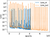 |
Fig. 1. Total neural network (NN) loss for the solution with λ = 20° and θpc = 36° in the closed line (blue) and open line (orange) regions versus training epochs. The differences in epochs arises from the varying number of steps taken by the training algorithm during second-order optimization. Training initially employed a first-order optimizer, which was switched to a second-order optimizer after 104 training epochs. Beyond that, we adjusted the shape of the interim separatrix every 3 × 10⁴ epochs, producing the blue and orange high spikes. The total training loss achieved, between 10−5 and 10−6, is considered satisfactory. |
Figs. 2 and 3 show two cross sections of the 3D solutions: one along the corotating xz plane that contains both the rotation and magnetic axes, and one along the corotating yz plane perpendicular to it. The initially dipolar separatrices are significantly stretched closer to the light cylinder. We also observe a clear nulling of the poloidal field Bp at the Y-point, where Bϕ is non-zero due to the return current flowing back to the star along the equatorial current sheet. This result was predicted by Uzdensky (2003) but has not been observed so clearly previously, mainly because until now no ideal force-free solution has obtained zero-thickness equatorial and separatrix current sheets. Uzdensky (2003) also predicted that because Bp = 0 and Bϕ ≠ 0 are immediately outside the Y-point, while Bϕ ≈ 0 immediately inside, Bp must be non-zero just inside the Y-point to achieve pressure balance between the interior and exterior at that point. Consequently, the shape of the Y-point must be a T, as clearly shown in Figs. 2 and 3. This feature has not been observed in previous numerical solutions, starting from Contopoulos et al. (1999), in which the separatrix was always shown with a pointed shape at the origin of the equatorial current sheet.
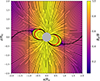 |
Fig. 2. Cross section of steady-state solution for an inclined rotator with λ = 20° and θpc = 36°, where r* = 0.25Rlc. The rotation axis aligns with the z axis and the inclined magnetic axis lies along the corotating xz plane. This cross section represents phase 0 (or π) of the corresponding rotating time-dependent solution. Closed thick black lines show the separatrix between open and closed field lines. Open thick black lines indicate the separatrix between open field lines that originate from the northern and southern magnetic poles, marking the location of the equatorial current sheet. Red lines show the initial dipolar shapes of the interim separatrices before readjustment. For this polar-cap choice, the dipole is significantly stretched outward toward the light cylinder (dashed lines at x/Rlc = ±1). The equatorial current sheet lies where lines from the north and south polar cap rim meet. The color scale shows the ratio Bp/B, representing the development of the azimuthal magnetic field Bϕ across the magnetosphere. At the magnetospheric Y-point, where the equatorial current sheet connects to the separatrix current sheet, Bp = 0 and Bϕ ≠ 0 as expected (Uzdensky 2003). In this solution, the Y-point remains significantly inside the light cylinder. |
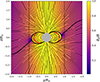 |
Fig. 3. Same as Fig. 2, but along the corotating yz plane. This cross section represents phase π/2 (or 3π/2) of the corresponding rotating time-dependent solution. |
Figs. 4 and 5 show the 3D distribution of open magnetic field lines immediately above and below the magnetospheric equatorial and separatrix current sheet. The value of α is numerically adjusted along each open field line so that it smoothly crosses the light cylinder. In particular, while Contopoulos et al. (1999) developed a complex numerical method to perform this adjustment, NNs accomplish it automatically. Fig. 5 shows the undulating shape of the equatorial current sheet beyond the closed line region. This corresponds to the boundary between the regions of open field lines that originate from the north and south magnetic poles. The undulating black lines in Figs. 2 and 3 are obtained from the intersection of the 3D undulating current sheet in Figs. 4 and 5 with the xz and yz planes, respectively.
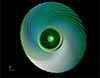 |
Fig. 4. Steady-state solution of Fig. 2 in 3D as seen from above. The yellow cylinder denotes the light cylinder and the pale undulating surface is the equatorial current sheet. Only open magnetic field lines just inside the rim of the northern polar cap are plotted. The Y-point in this solution lies significantly inside the light cylinder. The clear azimuthal break of open field lines is evident very close to the Y-point where Bp → 0 and Bϕ ≠ 0. |
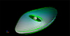 |
Fig. 5. The steady-state solution of Fig. 4 as seen from the side. Open magnetic field lines just inside the rims of both polar caps are plotted. The undulating shape of the equatorial current sheet between them is clearly visible. The solution does not develop the physical instabilities seen in all previous numerical solutions because this physics is not included in our method (we obtain the solution without a current sheet and then reverse the field direction in the southern magnetic hemisphere). |
Figure 6 shows that closed field lines develop a stronger azimuthal twist relative to the magnetic axis as they approach the separatrix. Nevertheless, in the closed line region we required that α = 0. Apparently, closed field lines must connect footpoints of equal potential to prevent electric currents from flowing along them. For an inclined rotator, these footpoints do not lie on the same stellar meridian, unlike in an axisymmetric rotator. This interesting result requires further investigation. In a non-rotating inclined dipole, the footpoints of closed magnetic field lines are not connected to each other. This raises the question of how initially dipolar closed magnetic field lines evolve in a time-dependent ideal simulation that involves the rotation of an initially static inclined dipole (as e.g., in Spitkovsky 2006, and thereafter). An ideal time-dependent simulation should preserve the same footpoints indefinitely. It remains unclear how these footpoints evolve in previous time-dependent ideal simulations. Fig. 7 shows the distribution of the electric current parameter α on the neutron star surface from above the rotation axis. The main magnetospheric current flows along the blue region where α < 0 for a pulsar with inclination λ < 90°, as in the present solution. The return current flows mainly along the separatrix (dotted black line) and partly in the yellow-red region inside the polar cap (compare with Fig. 4 of Bai & Spitkovsky 2010).
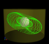 |
Fig. 6. Close-up of Fig. 5 near the stellar surface in the closed line region. This solution requires that α = 0 in this region. Nevertheless, the field lines develop a clear azimuthal twist with respect to the magnetic axis. |
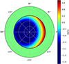 |
Fig. 7. Distribution of current parameter α along the stellar surface as seen from above the polar cap for the solution of Fig. 2. In the green closed line region outside the polar caps, α = 0. The azithmuthal angle ϕ = 0 lies along the corotating xz plane of Fig. 2 in the direction of inclination of the magnetic axis. The blue region shows the main magnetospheric current. The yellow-red region indicates part of the return current, with the main part of the return currently lying along the separatrix (thick dotted black line). |
Figure 8 shows the integral of the Poynting vector, E × B/(4π), over spheres of radius r centered on the star. Due to the absence of numerical current sheets, the total Poynting flux is almost conserved in the open line region, and we observe a slight numerical dissipation of around 10% out to 3Rlc. All previous numerical solutions show a clear drop in the integrated Poynting flux beyond the light cylinder as a result of dissipation at the equatorial current sheet. The total electromagnetic luminosity L is comparable to the estimate of Spitkovsky (2006), namely
 (7)
(7)
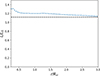 |
Fig. 8. Evolution with distance of the total Poynting flux L, calculated over spheres of radius r centered on the central star and normalized with respect to the aligned rotator’s canonical luminosity, L0 ≡ B*2r*6c/(4Rlc4). The value of L agrees with previous estimates in the literature (dashed line from Spitkovsky 2006 for the pulsar inclination angle considered). Energy is (almost) conserved beyond the Y-point and the light cylinder. |
from r ≈ 0.4Rlc to about 3Rlc. Here L0 = B*2r*6c/(4Rlc4) is the canonical aligned rotator’s luminosity value, and λ = 20° is the pulsar inclination angle. In Paper IV, we will compute a complete sequence of pulsar inclination angles, polar cap openings, and polar cap shapes. This will demonstrate whether the result of Paper II is reproduced in 3D, namely whether magnetospheric solutions exist even for arbitrarily small polar caps with luminosities L much smaller than the canonical value of Eq. (7).
4. Summary and conclusions
We have developed a robust numerical method that allows us to calculate steady-state force-free ideal 3D pulsar magnetospheres for various pulsar inclinations and polar cap shapes. Unlike all previous attempts, our method does not involve a time-dependent simulation that eventually relaxes to a steady-state. Instead, we directly solve the 3D generalization of the axisymmetric pulsar equation (Scharlemann & Wagoner 1973; Endean 1974; Mestel 1975). The method is not restricted to centrally located dipole fields and can accommodate more complex stellar magnetic field configurations.
For example, we can determine a particular magnetic field configuration that reproduces X-ray hotspot observations from the NICER satellite. These hotspots are assumed to correspond to the origin of open magnetic field lines (i.e., they are assumed to be the polar caps), enabling the calculation of the corresponding 3D ideal magnetosphere using our methodology. The initial field configuration reproducing these polar cap shapes requires inclusion of higher multipoles. Very small polar caps can be produced by slowly rotating inclined dipole and quadrupole fields (e.g. Gralla et al. 2017), while NICER hotspots require more complicated field structures with offset dipole and quadrupole configurations (Chen et al. 2020; Kalapotharakos et al. 2021). Although this complicates the initial ad hoc shape of the interim separatrix, as long as the polar caps remain fixed, the iteratively adjustable shape of the interim separatrix will remain topologically the same. We therefore expect our procedure to remain directly applicable and eventually converge to the true shape of the separatrix.
This methodology involves the decomposition of the pulsar magnetosphere into regions of open and closed field lines. This enables us to treat the separatrix current sheet as a perfect mathematical discontinuity between the two regions. We also “numerically remove” the equatorial current sheet by reversing the field direction in the southern hemisphere and restoring its true direction after the 3D solution is obtained. We acknowledge that although this approach facilitates numerical treatment of magnetospheric current sheets, it ignores the physics of reconnection, electromagnetic energy dissipation, plasma instabilities, and particle acceleration along them. In this sense, the solutions should be regarded as ideal solutions that require augmentation with the microphysics of current sheets. Our method can be directly applied to more general ideal MHD problems that contain current sheets, such as those in active regions of the solar corona. In this work we present our first solution for a particular (circular) polar cap size and shape of open magnetic field lines and a specific pulsar inclination angle relative to the rotation axis. The solution is obtained in a coordinate system that corotates with the star. Our results demonstrate the potential of the method to generate new solutions of the ideal pulsar magnetosphere.
We emphasize that the general steady-state ideal force-free solution is degenerate in the same sense as the axisymmetric solutions of Contopoulos (2005) and Timokhin (2006). In the axisymmetric case, the polar cap is circular, but its radial extent is arbitrary and depends on how far the closed line region extends from the light cylinder; a larger polar cap corresponds to a shorter closed line region. The solution in which the closed line region reaches the light cylinder is unique, and consequently the corresponding extent of the polar cap is also uniquely defined. In the present 3D case, not only is the size of the polar cap arbitrary, but also its shape and position. The solution obtained in this work corresponds to a circular polar cap centered around the magnetic axis. This choice causes the closed field line boundary to lie at different distances from the light cylinder as a function of azimuth and therefore does not correctly capture the field line sweepback at the polar cap. With the chosen inclination of 20°, this does not significantly affect the solution, but for larger inclination angles, it is expected to make a substantial difference.
We do not claim that this is the only ideal steady-state force-free solution of the pulsar magnetosphere. The general solution is clearly degenerate, and the configuration presented here represents only one valid solution. If we require the closed line region to reach the light cylinder everywhere, the resulting solution becomes unique and corresponds to a single polar cap shape that is neither circular nor centered around the magnetic axis. Multiple studies have shown that polar caps onto which previous time-dependent numerical simulations converge differ significantly from those of a static (or even retarded) vacuum dipole and depend on the magnetic inclination angle (e.g., Dyks & Harding 2004; Timokhin & Arons 2013).
In this paper, we trained two NNs that instantaneously yield the three components Bx, By, Bz of the magnetic field and their spatial derivatives at any given point (x, y, z) of the magnetosphere for one particular pulsar inclination, and one particular polar cap size and shape. This capability is extremely useful for visualizing magnetospheric features such as magnetic and electric field lines, charge, and current distributions, Poynting flux, and current sheets. We will present a detailed investigation of the pulsar magnetosphere for a range of pulsar inclinations and for various polar cap sizes and shapes in a forthcoming extended publication, along with the corresponding trained NNs (Paper IV). We also plan to investigate the unique solution in which the closed line region reached the light cylinder everywhere. Determining this unique solution will require adjustment of both the polar caps and the separatrix at each iteration step.
We aim to determine whether magnetospheric solutions exist even for arbitrarily small polar caps with correspondingly small luminosities, as suggested by the 2D results in (Paper II). We emphasize that our methodology allows us to obtain new ideal 3D pulsar-magnetosphere solutions by specifying various shapes and sizes of the polar cap a priori. Such solutions have not been obtained previously because existing numerical solutions approaches invariably relax to a single magnetospheric configuration, i.e., to a polar cap shape and size determined by the simulation itself, without any possibility for control by the programmer. Our approach opens up a broad spectrum of possible solutions through which a real pulsar magnetosphere may choose to transition during its evolution. Further work along these lines is warranted.
Data availability
The data underlying this article will be shared on reasonable request to the corresponding author.
Acknowledgments
This work was supported by computational time granted from the National Infrastructure for Research and Technology S.A. (GRNET) in the National HPC facility – ARIS – under project ID pr016005-gpu. ID is supported by the Hellenic Foundation for Research and Innovation (HFRI) under the 4th Call for HFRI PhD Fellowships (Fellowship Number: 9239). EC is supported by the Sectoral Development Program (OΠΣ 5223471) of the Ministry of Education, Religious Affairs and Sports of Greece, through the National Development Program (NDP) 2021-25.
References
- Bai, X.-N., & Spitkovsky, A. 2010, ApJ, 715, 1282 [Google Scholar]
- Bogovalov, S. V. 1999, A&A, 349, 1017 [Google Scholar]
- Bransgrove, A., Beloborodov, A. M., & Levin, Y. 2023, ApJ, 958, L9 [NASA ADS] [CrossRef] [Google Scholar]
- Cao, G., & Yang, X. 2022, ApJ, 925, 130 [Google Scholar]
- Cerutti, B., Philippov, A., Parfrey, K., & Spitkovsky, A. 2015, MNRAS, 448, 606 [Google Scholar]
- Chen, A. Y., Yuan, Y., & Vasilopoulos, G. 2020, ApJ, 893, L38 [Google Scholar]
- Contopoulos, I. 2005, A&A, 442, 579 [NASA ADS] [CrossRef] [EDP Sciences] [Google Scholar]
- Contopoulos, I., Kazanas, D., & Fendt, C. 1999, ApJ, 511, 351 [Google Scholar]
- Contopoulos, I., Pétri, J., & Stefanou, P. 2020, MNRAS, 491, 5579 [NASA ADS] [CrossRef] [Google Scholar]
- Contopoulos, I., Ntotsikas, D., & Gourgouliatos, K. 2024, MNRAS, 527, L127 [Google Scholar]
- Contopoulos, I., Dimitropoulos, I., Ntotsikas, D., & Gourgouliatos, K. N. 2024, Universe, 10, 178 [Google Scholar]
- Dimitropoulos, I., Contopoulos, I., Mpisketzis, V., & Chaniadakis, E. 2024, MNRAS, 528, 3141 [Google Scholar]
- Dyks, J., & Harding, A. K. 2004, ApJ, 614, 869 [Google Scholar]
- Endean, V. G. 1974, ApJ, 187, 359 [CrossRef] [Google Scholar]
- Goldreich, P., & Julian, W. H. 1969, ApJ, 157, 869 [Google Scholar]
- Gralla, S. E., Lupsasca, A., & Philippov, A. 2017, ApJ, 851, 137 [NASA ADS] [CrossRef] [Google Scholar]
- Hakobyan, H., Philippov, A., & Spitkovsky, A. 2023, ApJ, 943, 105 [NASA ADS] [CrossRef] [Google Scholar]
- Hewish, A. 1968, Sci. Am., 219, 25 [Google Scholar]
- Hu, R., & Beloborodov, A. M. 2022, ApJ, 939, 42 [NASA ADS] [CrossRef] [Google Scholar]
- Kalapotharakos, C., Brambilla, G., Timokhin, A., Harding, A. K., & Kazanas, D. 2018, ApJ, 857, 44 [NASA ADS] [CrossRef] [Google Scholar]
- Kalapotharakos, C., Wadiasingh, Z., Harding, A. K., & Kazanas, D. 2021, ApJ, 907, 63 [NASA ADS] [CrossRef] [Google Scholar]
- Lyubarskii, Y. E. 1990, Soviet Astronomy Letters, 16, 16 [Google Scholar]
- Mestel, L. 1975, Mem. Soc. Roy. Sci. Liege, 8, 79 [Google Scholar]
- Muslimov, A. G., & Harding, A. K. 2009, ApJ, 692, 140 [Google Scholar]
- Pétri, J. 2012, MNRAS, 424, 605 [Google Scholar]
- Philippov, A. A., Spitkovsky, A., & Cerutti, B. 2015, ApJ, 801, L19 [NASA ADS] [CrossRef] [Google Scholar]
- Scharlemann, E. T., & Wagoner, R. V. 1973, ApJ, 182, 951 [Google Scholar]
- Soudais, A., Cerutti, B., & Contopoulos, I. 2024, A&A, 690, A170 [NASA ADS] [CrossRef] [EDP Sciences] [Google Scholar]
- Spitkovsky, A. 2006, ApJ, 648, L51 [Google Scholar]
- Timokhin, A. N. 2006, MNRAS, 368, 1055 [Google Scholar]
- Timokhin, A. N., & Arons, J. 2013, MNRAS, 429, 20 [NASA ADS] [CrossRef] [Google Scholar]
- Uzdensky, D. A. 2003, ApJ, 598, 446 [NASA ADS] [CrossRef] [Google Scholar]
In axisymmetry, the current sheet may be fixed to lie along the boundary of the computational domain in the equator as in Contopoulos et al. (1999), while in 3D the position of the current sheet must be determined by the simulation. If one decides to simulate the full axisymmetric magnetosphere as in Cerutti et al. (2015), the same complication arises, since the current sheet is free to oscillate around the equator.
Without them, the negative surface charge density at the footpoint of the separatrix on the polar cap due to the electrons inflowing from the Y-point would be orders of magnitude higher than the expected electric field discontinuity accross the separatrix at that position.
Appendix A: Thickness of separatrix layer
We offer here a tentative explanation why, in all PIC simulations of the past decade, the separatrix current sheet turns out to be so much thicker than the equatorial current sheet.
Both current sheet are charged due to the discontinuity of the vertical electric field component across them (which is itself due to the discontinuity of the poloidal magnetic field, that is itself due to the presence of poloidal electric currents only in the open line region). We can thus also call them ‘charge sheets’. The question is what is the source of the electric charges needed to support both the charge and the electric current of the sheet. Regarding the equatorial current sheet, it is well accepted that relativistic reconnection takes place all along it, therefore, magnetospheric field lines enter it over an extended region beyond the Y-point. Each such field line carries electron-positron pairs with it which are thus introduced in the equatorial current sheet. Therefore, the supply of charges in the equator is ample. As a result, the equatorial current sheet can be really thin as is indeed seen in all previous PIC simulations.
This is not the case, however, with the separatrix surface. Reconnection along it is minor because this is not a Harris-type current sheet as the equatorial one (it contains a strong guide field), and there are no field lines entering it along the way from the stellar surface to its tip at the Y-point. One might think that the high density of magnetospherically supplied pairs that allowed the equatorial current sheet to appear so thin in the numerical PIC simulations will also supply the necessary pairs in the separatrix. Unfortunately these are not enough since, as we have shown in Contopoulos et al. (2020), an extra outward flow of positrons/protons is required through the separatrix to support the separatrix electric current and electric charge2. This flow of positive charges must originate on the stellar polar cap, where their charge density must accordingly be immense (a positronic current sheet corresponds also to a positronic charge sheet of infinite density-mathematically). In all previous PIC simulations, however, only a finite pair density on the order of the Goldreich-Julian value is introduced everywhere on the stellar surface. This is insufficient to support a current/charge sheet, therefore, the separatrix electric current is distributed over a wide region of poloidal field lines on the stellar surface. This effect eliminates the concept of a ‘separatrix surface’ and leads to the strange features observed in all previous PIC simulations, namely a thick separatrix and a region of strong dissipation just inside the light cylinder. We suspect that, if one introduces a much higher multiplicity of pairs on the stellar surface (e.g., 100 times the Goldreich-Julian value), the separatrix return current region will be correspondingly thinner (e.g., 100 times; see also Contopoulos et al. 2020). This would be a very interesting numerical experiment to perform that would justify our present approach of dividing the magnetosphere in the two regions of open and closed field lines separated by a separatrix surface (not the thick separatrix region of PIC simulations).
All Figures
|
Fig. 1. Total neural network (NN) loss for the solution with λ = 20° and θpc = 36° in the closed line (blue) and open line (orange) regions versus training epochs. The differences in epochs arises from the varying number of steps taken by the training algorithm during second-order optimization. Training initially employed a first-order optimizer, which was switched to a second-order optimizer after 104 training epochs. Beyond that, we adjusted the shape of the interim separatrix every 3 × 10⁴ epochs, producing the blue and orange high spikes. The total training loss achieved, between 10−5 and 10−6, is considered satisfactory. |
| In the text | |
|
Fig. 2. Cross section of steady-state solution for an inclined rotator with λ = 20° and θpc = 36°, where r* = 0.25Rlc. The rotation axis aligns with the z axis and the inclined magnetic axis lies along the corotating xz plane. This cross section represents phase 0 (or π) of the corresponding rotating time-dependent solution. Closed thick black lines show the separatrix between open and closed field lines. Open thick black lines indicate the separatrix between open field lines that originate from the northern and southern magnetic poles, marking the location of the equatorial current sheet. Red lines show the initial dipolar shapes of the interim separatrices before readjustment. For this polar-cap choice, the dipole is significantly stretched outward toward the light cylinder (dashed lines at x/Rlc = ±1). The equatorial current sheet lies where lines from the north and south polar cap rim meet. The color scale shows the ratio Bp/B, representing the development of the azimuthal magnetic field Bϕ across the magnetosphere. At the magnetospheric Y-point, where the equatorial current sheet connects to the separatrix current sheet, Bp = 0 and Bϕ ≠ 0 as expected (Uzdensky 2003). In this solution, the Y-point remains significantly inside the light cylinder. |
| In the text | |
|
Fig. 3. Same as Fig. 2, but along the corotating yz plane. This cross section represents phase π/2 (or 3π/2) of the corresponding rotating time-dependent solution. |
| In the text | |
|
Fig. 4. Steady-state solution of Fig. 2 in 3D as seen from above. The yellow cylinder denotes the light cylinder and the pale undulating surface is the equatorial current sheet. Only open magnetic field lines just inside the rim of the northern polar cap are plotted. The Y-point in this solution lies significantly inside the light cylinder. The clear azimuthal break of open field lines is evident very close to the Y-point where Bp → 0 and Bϕ ≠ 0. |
| In the text | |
|
Fig. 5. The steady-state solution of Fig. 4 as seen from the side. Open magnetic field lines just inside the rims of both polar caps are plotted. The undulating shape of the equatorial current sheet between them is clearly visible. The solution does not develop the physical instabilities seen in all previous numerical solutions because this physics is not included in our method (we obtain the solution without a current sheet and then reverse the field direction in the southern magnetic hemisphere). |
| In the text | |
|
Fig. 6. Close-up of Fig. 5 near the stellar surface in the closed line region. This solution requires that α = 0 in this region. Nevertheless, the field lines develop a clear azimuthal twist with respect to the magnetic axis. |
| In the text | |
|
Fig. 7. Distribution of current parameter α along the stellar surface as seen from above the polar cap for the solution of Fig. 2. In the green closed line region outside the polar caps, α = 0. The azithmuthal angle ϕ = 0 lies along the corotating xz plane of Fig. 2 in the direction of inclination of the magnetic axis. The blue region shows the main magnetospheric current. The yellow-red region indicates part of the return current, with the main part of the return currently lying along the separatrix (thick dotted black line). |
| In the text | |
|
Fig. 8. Evolution with distance of the total Poynting flux L, calculated over spheres of radius r centered on the central star and normalized with respect to the aligned rotator’s canonical luminosity, L0 ≡ B*2r*6c/(4Rlc4). The value of L agrees with previous estimates in the literature (dashed line from Spitkovsky 2006 for the pulsar inclination angle considered). Energy is (almost) conserved beyond the Y-point and the light cylinder. |
| In the text | |
Current usage metrics show cumulative count of Article Views (full-text article views including HTML views, PDF and ePub downloads, according to the available data) and Abstracts Views on Vision4Press platform.
Data correspond to usage on the plateform after 2015. The current usage metrics is available 48-96 hours after online publication and is updated daily on week days.
Initial download of the metrics may take a while.