| Issue |
A&A
Volume 705, January 2026
|
|
|---|---|---|
| Article Number | A61 | |
| Number of page(s) | 10 | |
| Section | Celestial mechanics and astrometry | |
| DOI | https://doi.org/10.1051/0004-6361/202555309 | |
| Published online | 07 January 2026 | |
Compact binary system dynamics at the second post-Newtonian order: Analytical formula of the coordinate time for eccentric and circular orbits
Ministero dell’Istruzione e del Merito (M.I.M., ex M.I.U.R.),
Italy
★ Corresponding authors: This email address is being protected from spambots. You need JavaScript enabled to view it.
; This email address is being protected from spambots. You need JavaScript enabled to view it.
Received:
26
April
2025
Accepted:
17
November
2025
Abstract
This work is based on our published letter, where we developed the analytical expression of the coordinate time in terms of the eccentric anomaly at the second post-Newtonian (PN) order in general relativity (GR) for a compact binary system moving on eccentric orbits. The aim of this paper is to provide more details about the performed calculations and to produce other new results. More specifically, we focus on deriving the analytical expression of the coordinate time at the second PN order for circular orbits, and then discuss two astrophysical applications involving binary neutron star and black hole systems.
Key words: gravitation / gravitational waves / methods: analytical / time / stars: black holes
© The Authors 2026
 Open Access article, published by EDP Sciences, under the terms of the Creative Commons Attribution License (https://creativecommons.org/licenses/by/4.0), which permits unrestricted use, distribution, and reproduction in any medium, provided the original work is properly cited.
This article is published in open access under the Subscribe to Open model. This email address is being protected from spambots. You need JavaScript enabled to view it. to support open access publication.
1 Introduction
General relativity (GR) is experiencing a flourishing epoch thanks to some breakthrough observational probes that have occurred in astrophysics in recent years, such as the direct detection of gravitational waves (GWs) from the merging of two black holes (BHs; Abbott et al. 2016), and from two neutron stars (NSs; Abbott et al. 2017), as announced by the Virgo and LIGO collaborations in 2015. In 2019, the first image of the supermassive BH located in the centre of the M87 galaxy was released by the Event Horizon Telescope collaboration (Event Horizon Telescope Collaboration 2019). However, other fundamental probes supporting GR have been confirmed over the years (Will 2014; Ishak 2019; Völkel et al. 2021).
These promising events do not stop scientists from inquiring into gravity; on the contrary, they encourage them to provide new solid tests. From an astrophysical perspective, gravity is still not fully understood in the strong field regime, and other alternatives must be considered. In this direction, one of the main targets for investigation is the class of compact binary systems.
From a theoretical point of view, these systems are very difficult to describe, because the non-linear structure of GR makes it even more difficult to derive the equations of motion (EoMs) (Blanchet 2014). However, even if we were able to determine them, they would be governed by retarded partial integrodifferential equations (Maggiore 2007; Blanchet 2014; Poisson & Will 2014), as compact objects are considered to be continuous bodies.
A practical way to solve this issue and, at the same time, to save the observational techniques developed in classical astronomy, is to resort to the post-Newtonian (PN) approximation method (Lorentz & Droste 1937). This approach is based on the following two crucial assumptions (Maggiore 2007; Blanchet 2014; Poisson & Will 2014): first, that the two bodies are slowly moving, weakly self-gravitating, and weakly stressed (also known as PN gravitational sources); second, that the two objects are well separated. In these hypotheses, we can first consider the bodies as two test particles and the curved background can be approximated as a Newtonian absolute Euclidean space, on which we can add the relativistic corrections in the power-series of 1/c (Blanchet 2014). In particular, the n PN order indicates that one expands a formula to order 1/c2n and neglects higher terms. The practical effect of this strategy consists of dealing with ordinary differential equations, which preserve their relativistic nature (i.e. invariance under a global PN-expanded Lorentz transformation; Blanchet 2014; Poisson & Will 2014). Instead, they lose the GR general covariance, as particular coordinate systems are employed (e.g. harmonic coordinates).
The PN technique is widely and successfully exploited in the astrophysical literature (Blanchet 2024), where the various fields of application are gravitational back-reaction in compact binary systems (Taylor & Weisberg 1989; Damour & Taylor 1991; Kramer et al. 2006, 2021); direct detection of GWs from coalescing compact binaries (Blanchet 2014); precision tests of gravity theories (Wex 2014); NS mass measurements in binary pulsars (Özel & Freire 2016); and investigation of the nature of extreme mass-ratio inspiral candidates (Amaro-Seoane 2018).
The focus of this work is on the BH binaries and relative emission of GWs, which are closely related and where the PN method is extensively employed. The state of the art on the conservative dynamics for non-spinning compact binaries is derived at the 4PN order, following different formalisms (Damour et al. 2014, 2016; Bernard et al. 2016; Marchand et al. 2018; Foffa & Sturani 2019; Foffa et al. 2019); it has also been extended to 5PN and 6PN levels, acknowledging that there are some unknown variables to be determined (Bini et al. 2019, 2020b,a, 2021). The GW templates, however, have been derived up to 4PN accuracy (Marchand et al. 2020; Larrouturou et al. 2022).
Finally, for spinning compact binaries, the effects in the radiative field and the energy flux are such that the spin-orbit (SO) contribution is known at 4 PN (Bohé et al. 2013; Marsat et al. 2014), whereas the spin-spin (SS; Bohé et al. 2015; Cho et al. 2021) and the spin-spin-spin (SSS; Marsat 2015) at 3PN; the SO, SS, and SSS interactions in the EoMs have been computed at 3.5PN (Damour et al. 2008; Marsat et al. 2013; Bohe et al. 2013; Levi & Steinhoff 2016), 3PN (Bohé et al. 2015; Levi & Steinhoff 2014; Cho et al. 2021), and 3.5PN level (Marsat 2015), respectively.
After the first GW detection occurred in 2015, more than 100 GW events have been observed from astrophysical compact binary mergers (examples are BH–BH, NS–NS, and looking for BH–NS candidates; Abbott et al. 2023; Soni et al. 2025). In addition, LIGO, Virgo, and KAGRA sensitivities have been updated so that the GW detection rate has been powered to be four times broader than the previous one, thus leading to the current fourth observational run (Cahillane & Mansell 2022; Soni et al. 2025). In this unstoppable observational GW detection survey, there will be other additional and complementary participants, represented by the future third-generation ground-based GW interferometers Einstein Telescope (Maggiore et al. 2020) and Cosmic Explorer (Reitze et al. 2019a,b), as well as the space-based devices LISA (Amaro-Seoane et al. 2017) and TianQin (Luo et al. 2016).
This unwavering drive to increase our observational capacity to investigate gravity and inspiralling BH binaries must be accompanied by appropriate theoretical assessments. This justifies the great excitement for achieving higher and higher PN orders. This is extremely helpful, both for extracting information on the gravitational source studied (Flanagan & Hughes 1998; Mingarelli 2019; Bernard et al. 2019; Soma et al. 2024), but also for generating template matching in ground- and space-based GW astronomy to fit observational data (Schmidt et al. 2024).
It is important to note that the GW signal h(T) is a parametric plot, having on the x-axis the coordinate time T related to the BH binary’s dynamics and on the y-axis the strain h(T) measured in the detector frame. Both functions, h(T) and T, depend on an angle parametrising the motion. Generally, the coordinate time is computed numerically, making production of the GW templates time-consuming and therefore the fit of the observational data arduous. Similarly, for pulsar timing, the pulse profile (depending on the coordinate time T) is computed numerically, thus allowing the development of suitable and elaborate algorithms to speed up the subsequent calculations.
The aim of this paper is to derive the analytical expression of the coordinate time T at the 2PN level as a function of the eccentric anomaly u. Therefore, providing T(u) allows us to have h(T(u)) as an analytical function, making the production of GW templates easier and faster, as well as the benchmark against observations. The same reasoning also applies to pulsar timing, as it drastically reduces the implementation of numerical schemes within software such as TEMPO (Taylor & Weisberg 1989), TEMPO2 (Edwards et al. 2006), and PINT (Luo et al. 2021). Moreover, it is applicable to coherent pulsar search algorithms (Lentati et al. 2018; Freire & Ridolfi 2018). This approach demonstrates substantial efficacy even at low PN orders, delivering tangible practical outcomes. The importance of this work lies primarily in the introduction of a novel methodology, absent from previous literature, that can be readily extended to higher PN orders.
This work provides more details on the derivation of the analytical expression of the coordinate time T at the 2PN level, already obtained in the letter (De Falco & Gallo 2025). In this regard, it is useful to recall that in a previous work (De Falco et al. 2023), De Falco and collaborators have derived the 1PN-accurate analytical formula of T(ϕ), where ϕ is the polar angle in the plane where the binary dynamics occurs. This result is obtained by considering the analytical formula of the relative distance R between the two bodies as a function of ϕ, namely R(ϕ), provided by Damour and Deruelle (Damour & Deruelle 1985). The derivation of T(ϕ), using the ϕ-parametrisation, is composed of three steps: determining the differential equation dT=f(ϕ) d ϕ, where f(ϕ) is the integrating function expressed up to the 1 PN level; analytically integrating the function f(ϕ); the final expression gives rise to a non-continuous function, as it shows periodic non-connected branches, not adapted to describe the coordinate time (being a monotonically increasing function). The cause of this effect is the presence of the tangent function, which appears in a non-linear way in the ensuing integrated formula. Therefore, to attain the continuity, we introduce the concept of accumulation function, which at every period smoothly connects the periodic curves to then have a regular map. The final result perfectly matches the coordinate time computed numerically.
In this paper, we show how to determine T(u) at the 2PN order as a function of the eccentric anomaly u. This time, the alternative u-parametrisation is due to the different orbit description offered by Schäfer and Wex at the 2PN order (Schäfer & Wex 1993). It is important to note that the authors do not provide an analytical expression of R(ϕ), as this expression is extremely demanding due to the equations involved, which turn out to be highly non-linear. Our analytical expression is the combination of various intertwined procedures, which will be better explained in this paper. The surprising result is that, up to the 1PN level, we do not need to invoke the accumulation function, whereas it must be necessarily exploited to work out the 2PN term. BH binary’s dynamics and related GW emission are breeding grounds for applying the 2PN coordinate time formula, where higher PN schemes are fundamental. Instead, for pulsar binary systems the 2PN contribution seems to be less essential1. However, through our analytical formula it is easier to fit the observational data and thus the extraction of the 2PN parameters related to the binary compact object under study. Indeed, having the two bodies’ masses, the relative distance, the relative radial velocity, and the orbital eccentricity, we are able to estimate the relativistic precession and reconstruct the orbital motion up to the 2PN order.
The paper is organized as follows: in Sect. 2 we provide the physics and mathematical setting related to the motion of compact binary systems; we first focus on the elliptic dynamics (see Sect. 3) and then on the circular orbits (see Sect. 4); we then provide two astrophysical applications of our formula (see Sect. 5); we finally draw the conclusions and future perspectives (see Sect. 6).
2 Compact binary system setting
We consider a compact binary system composed of two selfgravitating bodies with masses m1>m2, total mass M=m1+ m2, position vectors r1(T) and r2(T), and velocity vectors v1(T) and v2(T), where T is the coordinate time. Furthermore, we define the separation vector R(T)=r1(T)−r2(T) and its modulus R=|R(T)|, the reduced mass μ=m1 m2/M, the symmetric mass ratio v=μ/M, and the unit vector n=R(T)/R. Introducing r=R /(GM) and r=|r|, the coordinate time scales as t=T(GM) (Memmesheimer et al. 2004). The EoMs at the 2PN order in the centre-of-mass frame in harmonic coordinates are derived via the Hamiltonian formalism and read as (Memmesheimer et al. 2004; Schäfer & Wex 1993):
 (1a)
(1a)
 (1b)
where s=1/r, s−and s+are the inverse of the apastron and periastron, respectively2. The last quantities are determined by searching for the non-vanishing positive roots having finite limit as
(1b)
where s=1/r, s−and s+are the inverse of the apastron and periastron, respectively2. The last quantities are determined by searching for the non-vanishing positive roots having finite limit as  of the fifth-degree polynomial in Eq. (1a). The coefficients Aj, (see Eq. (A3a) in Memmesheimer et al. 2004) and Bj (see Eq. (A4a) in Memmesheimer et al. 2004), are functions of v, 2 PN energy
  , and reduced 2PN angular momentum
  , with h=J /(GM) and J being the angular momentum. The explicit expressions of E and h can be found in Memmesheimer et al. (2004). The EoMs can be written employing the following “Keplerian-like” parametrisation (Memmesheimer et al. 2004):
 (2a)
(2a)
 (2b)
(2b)
 (2c)
(2c)
![Mathematical equation: $v =2 \arctan \left[\left(\frac{1+e_{\varphi}}{1-e_{\varphi}}\right)^{1 / 2} \tan \frac{u}{2}\right],$](/articles/aa/full_html/2026/01/aa55309-25/aa55309-25-eq9.png) (2d)
where u and v are the eccentric and true anomalies, respectively, ϕ the polar angle, l=n(t−t0) the mean anomaly,
(2d)
where u and v are the eccentric and true anomalies, respectively, ϕ the polar angle, l=n(t−t0) the mean anomaly,  the mean motion with P the orbital period, ϕ0 and t0 the initial orbital phase and initial time, respectively. In (Eq. (2c)), the factor 2 π/K gives the angle of advance of the periastron per orbital revolution, where K is a function of v, E, h3. Finally, ar is the semi-major axis of the orbit, er, eϕ, et the PN eccentricities, and f4 ϕ, g4 ϕ, f4 t, g4 t some PN functions depending on v, E, h. The explicit expressions of all the aforementioned quantities can be found in Memmesheimer et al. (2004); Schäfer & Wex (1993).
Now, let us singularly analyse the system of Eq. (2). Equation (2a) is the parametrisation of the orbit (where ar has been divided by GM to agree with the definition of r); Eq. (2b) is the 2PN version of the Kepler equation; Eq. (2c) gives the equation connecting the polar angle with the true anomaly, where at the 2PN order v is not linearly linked to ϕ, as there is the addition of trigonometric functions of v weighted with some PN coefficients; eventually, Eq. (2d) gives the classical relation that exists between true and eccentric anomalies.
3 Elliptic case
We assume that the two bodies in the binary system move on eccentric orbits (i.e. er ≠ 0, et ≠ 0, eϕ ≠ 0). In this framework, we derive the analytical expression of the coordinate time t in terms of the eccentric anomaly u. This section is organized in three parts: we first derive the function pertaining to the time that must be integrated (see Sect. 3.1); in this derivation, we display the presence of infinite sums and how to treat them (see Sect. 3.2); after these preparatory steps, we show how to derive the analytical expression of the coordinate time up to the 2PN order (see Sect. 3.3).
3.1 Integrating function
The differential equation underlying the coordinate time is ruled by Eq. (1a). However, this form is not suitable yet, because we would obtain t(r). However, from the Keplerian-like parametrisation (2a), we have that r=r(u). This suggests first combining Eqs. (1a) and (1b) by introducing this helping function
 (3)
Knowing that s=s(u)=1/r(u), we arrive at
(3)
Knowing that s=s(u)=1/r(u), we arrive at
 (4)
where
(4)
where  , and deriving Eq. (2c) we have
![Mathematical equation: $\begin{align*} \frac{\mathrm{d} \varphi}{\mathrm{~d} u}= & \left(\frac{2 \pi}{K}\right)^{-1} \frac{\sqrt{1-e_{\varphi}^{2}}}{1-e_{\varphi} \cos u} \\ & \times\left[1+2 \frac{f_{4 \varphi}}{c^{4}} \cos (2 v)+3 \frac{g_{4 \varphi}}{c^{4}} \cos (3 v)\right]. \end{align*}$](/articles/aa/full_html/2026/01/aa55309-25/aa55309-25-eq14.png) (5)
Equation (4) cannot be still integrated, because in the above expression there is v, which can be linked to u via Eq. (2d). However, this simple substitution would provide a highly non-linear differential equation. For that reason, following the approach of Boetzel et al. (2017), Eq. (5) can be equivalently written as (see Appendix A for details)
(5)
Equation (4) cannot be still integrated, because in the above expression there is v, which can be linked to u via Eq. (2d). However, this simple substitution would provide a highly non-linear differential equation. For that reason, following the approach of Boetzel et al. (2017), Eq. (5) can be equivalently written as (see Appendix A for details)
![Mathematical equation: $\begin{align*} \cos (2 v)= & \frac{2-e_{\varphi}^{2}-2 \sqrt{1-e_{\varphi}^{2}}}{e_{\varphi}^{2}}+\frac{4 \sqrt{1-e_{\varphi}^{2}}}{e_{\varphi}^{2}} \\ & \times\left[\sum_{m=1}^{+\infty} \beta^{m}\left(m \sqrt{1-e_{\varphi}^{2}}-1\right) \cos (m u)\right], \end{align*}$](/articles/aa/full_html/2026/01/aa55309-25/aa55309-25-eq15.png) (6a)
(6a)
![Mathematical equation: $\begin{align*} \cos (3 v)= & \frac{3 e_{\varphi}^{2}-4+\left(4-e_{\varphi}^{2}\right) \sqrt{1-e_{\varphi}^{2}}}{e_{\phi}^{3}} \\ & +\frac{2 \sqrt{1-e_{\varphi}^{2}}}{e_{\varphi}^{3}}\left\{\sum _ { m = 1 } ^ { + \infty } \beta ^ { m } \left[2 m^{2}\left(1-e_{\varphi}^{2}\right)\right.\right. \\ & \left.\left.-6 m \sqrt{1-e_{\varphi}^{2}}+4-e_{\varphi}^{2}\right] \cos (m u)\right\}, \end{align*}$](/articles/aa/full_html/2026/01/aa55309-25/aa55309-25-eq16.png) (6b)
where
(6b)
where  . Therefore, to avoid dealing with non-linear expressions, we are forced to introduce infinite sums, which both depend directly on cos (mu) through some different coefficients.
3.2 Compact form of the infinite sums
We have seen that Eq. (6) introduces infinite sums in Eq. (4). However, this kind of representation is useless for application purposes, as they cannot be implemented in a numerical code. Therefore, we need to truncate them to a certain finite threshold mmax. This value strongly depends on the values of the input parameter and the tolerance we would like to achieve. The form of Eq. (6) is not helpful for our objectives. Therefore, we manipulate them by introducing a more compact expression given by
![Mathematical equation: $\begin{align*} \chi\left(m_{\max }\right)= & 2 \frac{f_{4 \varphi}}{c^{4}} \cos (2 v)+3 \frac{g_{4 \varphi}}{c^{4}} \cos (3 v) \\ = & \frac{1}{c^{4}}\left\{\sum_{m=1}^{m_{\max }}\left[2 f_{4 \varphi 0} x(m)+3 g_{4 \varphi} y(m)\right] \cos (m u)\right. \\ & \left.+2 f_{4 \varphi 0} x_{0}+3 g_{4 \varphi 0} y_{0}\right\}, \end{align*}$](/articles/aa/full_html/2026/01/aa55309-25/aa55309-25-eq18.png) (7)
where
(7)
where  is the 0PN eccentricity,
  , and the other coefficients read as
![Mathematical equation: $f_{4 \varphi 0} =\frac{e_{0}^{2}[v(19-3 v)+1]}{8 h_{0}^{4}},$](/articles/aa/full_html/2026/01/aa55309-25/aa55309-25-eq21.png) (8a)
(8a)
 (8b)
(8b)
 (8c)
(8c)
![Mathematical equation: $y(m) =\frac{\left[2 e_{1}\left(2 e_{1} m^{2}-3 \sqrt{2} m+e_{1}\right)+3\right]}{2 e_{0}\left(\sqrt{2} e_{1} m-1\right)} x(m),$](/articles/aa/full_html/2026/01/aa55309-25/aa55309-25-eq24.png) (8d)
(8d)
 (8e)
(8e)
![Mathematical equation: $y_{0} =\frac{e_{0}^{3}\left[3 e_{0}^{2}+\sqrt{2} e_{1}\left(2 e_{1}^{2}+3\right)-4\right]}{\left(1-2 e_{1}^{2}\right)^{3}}.$](/articles/aa/full_html/2026/01/aa55309-25/aa55309-25-eq26.png) (8f)
Since the problem is invariant with respect to time- and polar-angle shifts, we can set without loss of generality t0=0 and ϕ0=0. We fix the initial conditions as follows: R0=r(0) being the initial separation between the bodies; ṙ(0)=0 because we assume that the motion starts with no radial advance;
(8f)
Since the problem is invariant with respect to time- and polar-angle shifts, we can set without loss of generality t0=0 and ϕ0=0. We fix the initial conditions as follows: R0=r(0) being the initial separation between the bodies; ṙ(0)=0 because we assume that the motion starts with no radial advance;  , where
  is the initial orbital eccentricity. In this setting, the function χ depends only on γ (or e0) and r0.
The study of the truncation error related to the χ function can be easily performed via Eq. (7) through the introduction of the following function
 (9)
where Δ(0) means that we neglect all the infinite sum, that is, we have χ(0)=2 f4 ϕ 0 x0+3 g4 ϕ 0 y0. In Fig. 1, we display the function χ versus u for different values of mmax. Substituting in χ these expressions,
(9)
where Δ(0) means that we neglect all the infinite sum, that is, we have χ(0)=2 f4 ϕ 0 x0+3 g4 ϕ 0 y0. In Fig. 1, we display the function χ versus u for different values of mmax. Substituting in χ these expressions,  , and letting r0, γ, M free to vary, it is possible to check that χ depends only on r0 and γ (or equivalently from e0). To better understand the relation existing among Δ, r0, e0, we produce a 3D plot fixing the value of mmax and evaluating χ in u=π. It is important to note that the selected value of u corresponds to the maximum achieved by χ, as can be seen from Fig. 1. In Fig. 2, we conclude that high eccentricities e0 (or equivalently low initial orbit eccentricities γ) are responsible for the increment of the truncation error, whereas higher initial distances r0 make it lower.
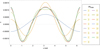 |
Fig. 1 Plot of function χ versus eccentric anomaly u ∈[0, 2 π] for different values of mmax=1, …, 15. |
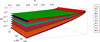 |
Fig. 2 3D plot showing link among Δ(i), r0, e0 for ten different fixed values of mmax. |
3.3 Analytical expression
In this section, we explain how to obtain the analytical expression of the coordinate time at 2 PN order. We structure the argument in these five parts: we first write down the integrating function (see Sect. 3.3.1); then we easily obtain the coordinate time at 1PN order (see Sect. 3.3.2); as a further step, we work out the 2PN term (see Sect. 3.3.3), which requires introducing the concept of accumulation function to make t(u) a smooth function (see Sect. 3.3.4); finally, we study the accuracy of the analytical formula determined (see Sect. 3.3.5).
3.3.1 General setting
The integrating function τ(u) (cf. Eq. (4)) can be split at the various PN orders as follows:
 (10)
The analytical formula for the coordinate time as a function of u is obtained by solving the following integrals:
(10)
The analytical formula for the coordinate time as a function of u is obtained by solving the following integrals:
![Mathematical equation: $\begin{align*} t(u) & =\int\left[\tau_{0 \mathrm{PN}}(u)+\frac{1}{c^{2}} \tau_{1 \mathrm{PN}}(u)+\frac{1}{c^{4}} \tau_{2 \mathrm{PN}}(u)\right] \mathrm{d} u \\ & =t_{0 \mathrm{PN}}(u)+\frac{1}{c^{2}} t_{1 \mathrm{PN}}(u)+\frac{1}{c^{4}} t_{2 \mathrm{PN}}(u) \end{align*}$](/articles/aa/full_html/2026/01/aa55309-25/aa55309-25-eq32.png) (11)
(11)
The numerical integration of Eq. (11) presents a monotonically increasing trend, as we expect (De Falco et al. 2023). Instead, the analytical solution t(u) can be derived by explicitly computing the three integrals in Eq. (11).
3.3.2 1PN formula
The first two terms in Eq. (11) are easily integrated, thus providing the 1PN formula of the coordinate time
 (12a)
(12a)
![Mathematical equation: $\begin{align*} t_{1 \mathrm{PN}}(u)= & \frac{1}{8 \sqrt{2} e_{0}\left(-E_{0}\right)^{5 / 2}}\left\{E _ { 0 } ^ { 2 } \left[8 h_{0} h_{1}+4 e_{1}^{2}(3 v-1)\right.\right. \\ & -7(v+1)] \sin u+2 e_{1}\left(4 e_{1}^{2}-3\right) \sin u \\ & \left.+e_{0} u\left[6 E_{1}-E_{0}^{2}(v-15)\right]\right\}. \end{align*}$](/articles/aa/full_html/2026/01/aa55309-25/aa55309-25-eq35.png) (12b)
We note that this result recovers the one proposed in our previous work4 (De Falco et al. 2023). The main difference relies on the employment of the angle ϕ, inspired by the analytical expression R(ϕ) provided by Damour & Deruelle (Damour & Deruelle 1985). However, this approach leads to discontinuous trigonometric functions. We can build up a smooth coordinate time by resorting to the accumulation function, which regularly connects the periodic branches. Here, we circumvent the issue by exploiting the angle u, which directly yields a smooth function at 1PN order.
(12b)
We note that this result recovers the one proposed in our previous work4 (De Falco et al. 2023). The main difference relies on the employment of the angle ϕ, inspired by the analytical expression R(ϕ) provided by Damour & Deruelle (Damour & Deruelle 1985). However, this approach leads to discontinuous trigonometric functions. We can build up a smooth coordinate time by resorting to the accumulation function, which regularly connects the periodic branches. Here, we circumvent the issue by exploiting the angle u, which directly yields a smooth function at 1PN order.
3.3.3 2PN formula
Finally, we need to determine only the 2PN contribution t2 PN, which can be written as
![Mathematical equation: $\begin{align*} \int \tau_{2 \mathrm{PN}}(u) \mathrm{d} u= & C\left[\sum_{i=0}^{3} a_{i} \mathcal{I}(i, 1)+\sum_{i=0}^{4} b_{i} \mathcal{I}(i, 2)\right. \\ & \left.+\sum_{i=0}^{5} c_{i} \mathcal{I}(i, 3)+\sum_{i=2}^{m_{\max }} d_{i} \mathcal{J}(i)\right], \end{align*}$](/articles/aa/full_html/2026/01/aa55309-25/aa55309-25-eq36.png) (13)
where the coefficients C, ai, bi, ci, di depend on v, E, h and can be found in De Falco & Gallo (2025), whereas
(13)
where the coefficients C, ai, bi, ci, di depend on v, E, h and can be found in De Falco & Gallo (2025), whereas
![Mathematical equation: $\mathcal{I}(n, m) =\int \frac{\cos ^{n} u \mathrm{~d} u}{\left[-e_{0}+\left(1-2 e_{1}\right) \cos u\right]\left(1-e_{0} \cos u\right)^{m}}$](/articles/aa/full_html/2026/01/aa55309-25/aa55309-25-eq37.png) (14a)
(14a)
![Mathematical equation: $\mathcal{J}(n) =\int \frac{\cos (n u) \mathrm{d} u}{\left[-e_{0}+\left(1-2 e_{1}\right) \cos u\right]\left(1-e_{0} \cos u\right)}$](/articles/aa/full_html/2026/01/aa55309-25/aa55309-25-eq38.png) (14b)
After the integration process, we obtain
(14b)
After the integration process, we obtain
 (15)
with
(15)
with
![Mathematical equation: $\mathcal{A}_{1}=\arctan \left[\sqrt{\frac{1+e_{0}}{1-e_{0}}} \tan \left(\frac{u}{2}\right)\right],$](/articles/aa/full_html/2026/01/aa55309-25/aa55309-25-eq40.png) (16a)
(16a)
![Mathematical equation: $\mathcal{A}_{2}=\arctan \left[\sqrt{\frac{e_{0}-2 e_{1}+1}{e_{0}+2 e_{1}-1}} \tan \left(\frac{u}{2}\right)\right].$](/articles/aa/full_html/2026/01/aa55309-25/aa55309-25-eq41.png) (16b)
The coefficients D1, D2, D3 are listed in De Falco & Gallo (2025).
(16b)
The coefficients D1, D2, D3 are listed in De Falco & Gallo (2025).
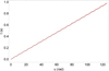 |
Fig. 3 Numerical integration of T(u) (black line) and analytical formula (red dashed line) with u ∈[0, 40 π]. The following parameter values have been used: m1=1.60 M⊙, m2=1.17 M⊙, γ=0.7, R0= r0(GM)=100 M, and ṙ(0)=0. The infinite sums have been truncated at mmax=10. |
3.3.4 Accumulation function
We note that 𝒜1 and 𝒜2 both have discontinuous periodic branches. Therefore, we need to resort to accumulation functions to obtain a smooth coordinate time. It is easy to check that 𝒜1 and 𝒜2 both share the same accumulation function, which reads as
![Mathematical equation: $ F(u)= \begin{cases}0 & \text { if } u \in[0, \pi],\\ \pi\left\{\left[\frac{u-\pi}{2 \pi}\right]+1\right\} & \text { otherwise, }\end{cases} $](/articles/aa/full_html/2026/01/aa55309-25/aa55309-25-eq42.png) (17)
where the symbol [·] in the above expression represents the integer part. Therefore, the continuous functions are
(17)
where the symbol [·] in the above expression represents the integer part. Therefore, the continuous functions are
 (18)
Therefore, the final 2PN contribution (15) reads as
(18)
Therefore, the final 2PN contribution (15) reads as
 (19)
(19)
3.3.5 Accuracy of the analytical formula
By substituting Eqs. (12a), (12b), (19) into Eq. (11), we finally retrieve the analytical expression of the coordinate time at the 2PN order in terms of u. To check the accuracy of our analytical formula with respect to the numerical integration of Eq. (11), we produce the plot reported in Fig. 3, where we note a good agreement5. The mean relative error, defined as the difference of the numerical and analytical expressions in modulus over the absolute value of the numerical formula, for our input parameters, and selecting mmax=10, amounts to 0.3%. We have chosen a high value of mmax as an example, to show the power of the compact form (7).
4 Circular case
In this section, we analyse the particular situation where the two bodies move on circular orbits. This case is realised by setting er=et=eϕ=0 (see Eqs. (26a) and (26b) in Memmesheimer et al. 2004). This implies that the Keplerian circular orbit parametrisation (2) becomes
 (20)
It is easy to check that f4 t=g4 t=f4 ϕ=g4 ϕ=0 (Memmesheimer et al. 2004).
(20)
It is easy to check that f4 t=g4 t=f4 ϕ=g4 ϕ=0 (Memmesheimer et al. 2004).
Based on these premises, τ(u) is independent of u (cf. Eq. (4)), as s=1/r does not depend on u, so also ψ(u) is independent of u. Furthermore, we have
 (21)
Therefore, we can write dt = 𝒯 du, where 𝒯 is a constant value that depends only on v, E, h, which reads as:
(21)
Therefore, we can write dt = 𝒯 du, where 𝒯 is a constant value that depends only on v, E, h, which reads as:
![Mathematical equation: $\begin{align*} \mathcal{T}= & \frac{G M}{4 E_{0}^{2} h_{0}}\left\{1+\frac{2 E_{1} h_{0}^{2}+E_{0}\left(h_{0} h_{1}-3\right)}{c^{2} e_{1}^{2}}\right. \\ & +\frac{1}{4 c^{4} e_{1}^{4}}\left[8 e_{1}^{2} h_{0}\left(E_{2} h_{0}-E_{1} h_{1}\right)+12 E_{1}\left(E_{1} h_{0}^{4}+2 e_{1}^{2}\right)\right. \\ & +4 e_{1}^{2} E_{0} h_{0} h_{2}+16 e_{1}^{6} E_{0}^{2} v(2 v+3)+2 e_{1}^{2} E_{0}^{2}(62 v-47) \\ & +4 E_{0}^{2} h_{0} h_{1}\left(h_{0} h_{1}-9\right)-e_{1}^{4} E_{0}^{2}\left(17 v^{2}+216 v-47\right) \\ & \left.\left.-15 E_{0}^{2}(2 v-7)\right]\right\}. \end{align*}$](/articles/aa/full_html/2026/01/aa55309-25/aa55309-25-eq47.png) (22)
Since t(u)=𝒯u, the coordinate time displays a linear trend in terms of u, where the slope is given by 𝒯.
(22)
Since t(u)=𝒯u, the coordinate time displays a linear trend in terms of u, where the slope is given by 𝒯.
For a circular orbit, the orbital period P can be computed as P=2 π 𝒯. It is also interesting to calculate the mean motion  , which reads as:
![Mathematical equation: $\begin{align*} n= & \frac{1}{G M h_{0}}\left\{-4 e_{1}^{2} E_{0}+\frac{4}{c^{2}}\left(E_{0}^{2} h_{0} h_{1}-2 E_{1} e_{1}^{2}\right)\right. \\ & +\frac{1}{c^{4}}\left[4 E_{1}^{2} h_{0}^{2}+8 E_{0} E_{1} h_{0} h_{1}-8 E_{2} e_{1}^{2}+4 E_{0}^{2} h_{0} h_{2}\right. \\ & +16 E_{0}^{3} e_{1}^{4} v(2 v+3)+16 E_{0}^{3}(7 v-4)-E_{0}^{3} e_{1}^{2}\left(17 v^{2}\right. \\ & +216 v-47)]\}. \end{align*}$](/articles/aa/full_html/2026/01/aa55309-25/aa55309-25-eq49.png) (23)
The case of quasi-circular orbits (generally present in some astrophysical scenarios; Alcubierre et al. 2005; Lorimer 2008) can either be computed by resorting to the coordinate time of the elliptic motion (low eccentricity, e0 ≪ 1), or can be directly approximated with that of the circular orbit case (zero eccentricity, e0=0). This choice strongly relies on the input values and the accuracy we need to achieve.
(23)
The case of quasi-circular orbits (generally present in some astrophysical scenarios; Alcubierre et al. 2005; Lorimer 2008) can either be computed by resorting to the coordinate time of the elliptic motion (low eccentricity, e0 ≪ 1), or can be directly approximated with that of the circular orbit case (zero eccentricity, e0=0). This choice strongly relies on the input values and the accuracy we need to achieve.
5 Astrophysical applications
We provide two astrophysical applications of Eq. (11): one related to binary NSs (see Sect. 5.1), and the other to binary BHs (see Sect. 5.2). Our formula allowed us to calculate the orbital period P associated with a compact binary system by assigning as input data: m1, m2, R0, e06. We note that another relevant input parameter is represented by the initial radial velocity ṙ0, which we approximated as zero. Its value can be computed from the differential form of Kepler’s third law, since the orbital motion remains Keplerian-like at any instant (De Falco et al. 2025):
 (24)
where Ṗ denotes the orbital period derivative. The compact binary systems that we considered show a Ṗ that typically lies in the range [10−19, 10−12], producing ṙ0 of the order [10−10, 10−7]. Such values can reasonably be assumed to be negligible, thus justifying our assumption ṙ0 ≈ 0.
(24)
where Ṗ denotes the orbital period derivative. The compact binary systems that we considered show a Ṗ that typically lies in the range [10−19, 10−12], producing ṙ0 of the order [10−10, 10−7]. Such values can reasonably be assumed to be negligible, thus justifying our assumption ṙ0 ≈ 0.
The orbital separation for eccentric binaries was estimated as the apastron distance, namely R0=a(1+e), where the semimajor axis length a was computed by again employing Kepler’s third law, yielding a=[GMP2 /(2 π)]1/3. These two remarks permitted us to reduce the input data to only three, namely m1, m2, e0.
We used our 2PN coordinate time formula (using mmax=10) to determine the companion mass for NS binaries and the orbital period for BH binaries. In both cases, we confirmed our theoretical values (denoted by an overbar, e.g.  , P̄) by benchmarking them against the observed ones reported in the literature.
5.1 Binary neutron stars
As reported in Nair & Stevenson (2025), more than 30 Galactic double NS (DNS) binaries have been identified in total through radio pulsar timing, while the number of systems with reliably measured total masses amounts to about 24 of those in the Galactic field. We selectes six DNS sources, and we used the observational data to test Eq. (11), because our 2PN formula allowed us to infer the companion mass m2. In addition, we estimated the secular periastron advance parameter  defined as
  (Kramer et al. 2021).
Among the selected DNS systems, we first considered the Hulse-Taylor gravitational source (also known as PSR B1913+16), composed of a NS and a pulsar. This is the most famous binary system, as it was not only the first to be discovered, but also provided an important confirmation of GR (Taylor & Weisberg 1982). Indeed, it has been shown that the observed orbital decay is consistent with the loss of energy due to the GW emission in GR. We chose other five candidates: PSR J0737-3039, the first detected binary pulsar (Kramer et al. 2021); PSR J0453+1559, another pulsar-NS asymmetric DNS, having the lightest known NS as companion (Martinez et al. 2015); PSR J0509+3801, formed by a pulsar and NS, moving on highly eccentric orbits, similarly to the Hulse-Taylor pulsar (Martinez et al. 2015); PSR J0514-4002A, composed of a millisecond pulsar and a massive white dwarf (WD) companion (McEwen et al. 2024; Ding et al. 2024), and finally PSR J1518+4904, formed by a pulsar and NS (Janssen et al. 2008).
In Table 1 we list all the input parameters related to the aforementioned DNS systems and the quantities we calculated. It can be seen that there is good agreement between the observed values and those computed with our formula. In fact, calculating the mean relative error, it is ∼ 2 × 10⁻³%. It is important to note that for some systems it would be possible to improve the accuracy of our predictions by considering that the bodies also are spinning, since there are relativistic spin precession effects that we did not actually take into account.
Among the ∼ 3600 pulsars identified in the Milky Way, a substantial subset resides in binary systems, most commonly with WD companions. Estimates place the Galactic population of pulsar-WD binaries at roughly 200 (Lorimer & Kramer 2012; Tauris & van den Heuvel 2023). We applied Eq. (11) to this class, which is dynamically less relativistic than the previously considered cases, to highlight the robustness of our formulation. In Table 2, we report the input parameters of some pulsar-WD systems. In this case, we estimated only the companion mass, because the observability of the relativistic precession advance strongly depends on the orbital eccentricity. For the majority of pulsar-WD binaries with nearly circular orbits, it is not measurable, whereas in rare eccentric systems it provides a powerful test of GR. In this case, we also noted a very good agreement between our theoretical predictions and the observational data, as the mean relative error was ∼ 10−3%. Since the eccentricities of these systems are very small, we checked our results also employing Eq. (22), which led to a mean relative error of 2% with respect to the eccentric 2PN formula. We stress that Eq. (11) is too accurate for the aforementioned binary systems, as they present mild relativistic effects.
Input parameters related to six selected DNS systems, together with quantities estimated by us.
Parameters of selected NS-WD binaries together with relative difference between companion mass values.
5.2 Binary black holes
We now consider eccentric, non-spinning BH binaries, following Ficarra & Lousto (2025). That study presents a systematic numerical relativity analysis, aimed at refining simulation strategies and assessing the impact of eccentricity and mass ratio on merger times and gravitational waveforms, ultimately contributing to the construction of a waveform catalogue for GW astronomy. Using the Einstein Toolkit, the authors performed 30 simulations covering mass ratios up to m1/m2=8.5 and initial eccentricities as large as e0 ≈ 0.45. The main diagnostic is the merger time, the coordinate instant when a common horizon emerges, normalised to its quasi-circular counterpart. From these runs, they extracted the relevant parameters, summarised in Table VII of Ficarra & Lousto (2025).
We selected six simulations reported in Table 3. In all cases, we set the total mass of the system to M=20 M⊙. However, the subsequent analysis was independent of this number, since all quantities were scaled by the total mass of the system, as required by general covariance. The orbital period was calculated using Kepler’s third law:
 (25)
(25)
As can be noted, the values estimated using our formula agree with those reported in the literature, with a mean relative accuracy of about 4%, further confirming the predictive power of our approach.
Input parameters for BH binaries taken from Ficarra & Lousto (2025), together with estimation of orbital period.
6 Conclusions
In this paper, we provide further details on the derivation of the analytical expression for the coordinate time (19), previously introduced in De Falco & Gallo (2025). Our guiding strategy is to follow the orbital parameterisation given in Eq. (2). We note that the inclusion of 2PN effects renders the classical and 1PN equations of celestial mechanics highly non-linear. These effects are encoded in the coefficients f4 ϕ, g4 ϕ, f4 t, g4 t, which are accompanied by trigonometric functions of the true anomaly v, which is itself non-linearly dependent on the eccentric anomaly u. This intricate structure prevents us from deriving an analytical expression for the relative separation radius R as a function of ϕ. We only have R(u), given a priori.
The first step is to derive the differential equation that governs the coordinate time, which can be written as dT=f(u), du, where f(u) is expanded up to 2PN order. Starting from Eq. (1b) and expressing it in terms of the inverse radius s, together with the parametrisation (2d), we still obtain d ϕ. Therefore, calculating the Jacobian of the transformation d ϕ/du, it seems that we have found the desired integrating function. However, the last term involves only v, which is not a simple function of u. A non-trivial procedure allows one to express the last term as an infinite series of trigonometric functions of u (see Eq. (6) and Appendix A for details). After some lengthy algebraic manipulations and 2PN expansions, we finally obtain the aforementioned differential equation.
In general, the procedure mentioned above to obtain the differential equation for the coordinate time could require long calculations, but it should also lead straightforwardly to its derivation. In particular, from the 2PN order onward, it will be more and more arduous to achieve this objective for the appearance of non-linear PN effects in the orbit parametrisation. In this work, we learned how to overcome the delicate issue of the nonlinearities existing between v and u using the method discussed in Appendix A. In particular, we expressed such infinite sums in a more compact form through Eq. (7), which must be truncated to a certain finite value mmax for application purposes. In addition, we showed how to properly estimate mmax once the input parameters are assigned and the accuracy error is chosen.
We stress that this preparatory part is fundamental for proceeding with the next steps, which are then expected to include a series of other demanding computations. In fact, once we obtain the function f(u), we can integrate it. We note that up to the 1PN order, it does not present discontinuities, as instead they occur whether or not we employ the ϕ-parametrisation and the analytical expression R(ϕ) (Damour & Deruelle 1985; De Falco et al. 2023). However, the 2PN term presents the appearance of two tangent functions and so the occurrence of discontinuities. This issue was solved via the accumulation function to make the overall formula regular.
This work presents two important results under a theoretical perspective in the GR PN literature: (1) the derivation of a more accurate formula for the coordinate time; (2) the refinement of a strategy from the 1PN to the 2PN order, which permits us to gather the differential equation for the coordinate time, handle the presence of infinite sums, and deal with discontinuous trigonometric maps via the accumulation function.
These aspects have never been treated in the literature by other authors. The developed methodology can be used broadly in other research fields, which share the same starting hypotheses of the problem we studied.
As we also underlined in the introduction, our formula is useful for computing the orbital period of compact binary systems during the inspiral stage, as well as to fit the observational data to extract information from the gravitational sources under study. We focus mainly on BH systems, as they normally feature considerable masses (and so also strong gravitational fields), which have a great impact on the 2PN term.
In addition, we point out that we derived T(u), but through Eq. (2c) it is also possible to obtain T(ϕ). In the latter case, we should be aware that we are adding a discontinuity, so we must resort to an accumulation function. In applications, it could happen that we need u(T) or ϕ(T). As the problem is formulated, we deem it extremely complicated to determine such analytical formulae. However, we can still employ T(u) or T(ϕ) and invert them numerically via an interpolation procedure, which generally is not so computationally expansive.
As already stressed initially, the actual and near future upgrades of our observational capacities and sensitivities motivate us to improve the order of the PN expansions. This activity at higher and higher PN orders is fundamental, not only for the practical result but also because it allows one to determine more about PN effects on the coordinate time and about the existence of new advantageous parametrisation, which could avoid the intervention of the accumulation function.
Our future perspectives aim at extending the present work to 3PN conservative dynamics and also to spinning binary systems. Regarding the latter topic, we have already worked in this direction, as we discovered a formal analogy existing between the GR and Einstein-Cartan theory at 1PN order (De Falco & Battista 2023). Indeed, we were able to formally relate the quantum spin effects with the macroscopic angular momentum, being thus able to switch between the two cases, depending on the problem under study.
It would also be stimulating to see how this approach changes depending on the addition of dissipative GW effects, and what kinds of new mathematical challenges will emerge (Blanchet 2024). Finally, another interesting avenue would be to extend our approach to the merger and ringdown stages, where the new effective-one-body model must be employed (Buonanno & Damour 1999, 2000; Damour & Nagar 2011). In this case, the technique presented in this work must be strongly refined, as the involved calculations will surely become more complicated and new fascinating issues may arise.
Acknowledgements
VDF is grateful to Gruppo Nazionale di Fisica Matematica of Istituto Nazionale di Alta Matematica for support. VDF acknowledges the support of INFN sez. di Napoli, iniziative specifiche TEONGRAV. The authors are grateful to Alessandro Ridolfi and Delphine Perrodin for the useful discussions and suggestions.
References
- Abbott, B. P., Abbott, R., Abbott, T. D., et al. 2016, Phys. Rev. Lett., 116, 061102 [Google Scholar]
- Abbott, B. P., Abbott, R., Abbott, T. D., et al. 2017, Phys. Rev. Lett., 119, 161101 [Google Scholar]
- Abbott, R., Abbott, T. D., Acernese, F., et al. 2023, Phys. Rev. X, 13, 041039 [Google Scholar]
- Alcubierre, M., Brügmann, B., Diener, P., et al. 2005, Phys. Rev. D, 72, 044004 [Google Scholar]
- Amaro-Seoane, P. 2018, Liv. Rev. Relativ., 21, 4 [NASA ADS] [CrossRef] [Google Scholar]
- Amaro-Seoane, P., Audley, H., Babak, S., et al. 2017, arXiv e-prints [arXiv:1702.00786] [Google Scholar]
- Bailes, M., Ord, S. M., Knight, H. S., & Hotan, A. W., 2003, ApJ, 595, L49 [Google Scholar]
- Bernard, L., Blanchet, L., Bohé, A., Faye, G., & Marsat, S. 2016, Phys. Rev. D, 93, 084037 [Google Scholar]
- Bernard, L., Cardoso, V., Ikeda, T., & Zilhão, M., 2019, Phys. Rev. D, 100, 044002 [Google Scholar]
- Bini, D., Damour, T., & Geralico, A., 2019, Phys. Rev. Lett., 123, 231104 [Google Scholar]
- Bini, D., Damour, T., & Geralico, A. 2020a, Phys. Rev. D, 102, 024061 [Google Scholar]
- Bini, D., Damour, T., & Geralico, A. 2020b, Phys. Rev. D, 102, 084047 [Google Scholar]
- Bini, D., Damour, T., Geralico, A., Laporta, S., & Mastrolia, P., 2021, Phys. Rev. D, 103, 044038 [Google Scholar]
- Blanchet, L., 2014, Liv. Rev. Relativ., 17, 2 [NASA ADS] [CrossRef] [Google Scholar]
- Blanchet, L., 2024, Liv. Rev. Relativ., 27, 4 [NASA ADS] [CrossRef] [Google Scholar]
- Boetzel, Y., Susobhanan, A., Gopakumar, A., Klein, A., & Jetzer, P., 2017, Phys. Rev. D, 96, 044011 [Google Scholar]
- Bohé, A., Marsat, S., & Blanchet, L., 2013, Class. Quant. Grav., 30, 135009 [Google Scholar]
- Bohe, A., Marsat, S., Faye, G., & Blanchet, L., 2013, Class. Quant. Grav., 30, 075017 [CrossRef] [Google Scholar]
- Bohé, A., Faye, G., Marsat, S., & Porter, E. K., 2015, Class. Quant. Grav., 32, 195010 [Google Scholar]
- Buonanno, A., & Damour, T., 1999, Phys. Rev. D, 59, 084006 [Google Scholar]
- Buonanno, A., & Damour, T., 2000, Phys. Rev. D, 62, 064015 [Google Scholar]
- Cahillane, C., & Mansell, G., 2022, Galaxies, 10, 36 [Google Scholar]
- Cho, G., Pardo, B., & Porto, R. A., 2021, Phys. Rev. D, 104, 024037 [CrossRef] [Google Scholar]
- Colwell, P., 1993, Solving Kepler’s Equation Over Three Centuries (Willmann-Bell) [Google Scholar]
- Damour, T., & Deruelle, N., 1985, Ann. Inst. Henri Poincaré Phys. Théor, 43, 107 [Google Scholar]
- Damour, T., & Nagar, A., 2011, Fundam. Theor. Phys., 162, 211 [Google Scholar]
- Damour, T., & Taylor, J. H., 1991, ApJ, 366, 501 [NASA ADS] [CrossRef] [Google Scholar]
- Damour, T., Jaranowski, P., & Schäfer, G., 2008, Phys. Rev. D, 77, 064032 [Google Scholar]
- Damour, T., Jaranowski, P., & Schäfer, G., 2014, Phys. Rev. D, 89, 064058 [Google Scholar]
- Damour, T., Jaranowski, P., & Schäfer, G., 2016, Phys. Rev. D, 93, 084014 [Google Scholar]
- De Falco, V., & Battista, E., 2023, Phys. Rev. D, 108, 064032 [Google Scholar]
- De Falco, V., & Gallo, M., 2025, Phys. Lett. B, 865, 139484 [Google Scholar]
- De Falco, V., Battista, E., & Antoniadis, J., 2023, Europhys. Lett., 141, 29002 [Google Scholar]
- De Falco, V., Carleo, A., Ridolfi, A., & Corongiu, A., 2025, A&A, 696, A49 [NASA ADS] [CrossRef] [EDP Sciences] [Google Scholar]
- Ding, H., Deller, A. T., Swiggum, J. K., et al. 2024, ApJ, 970, 90 [NASA ADS] [CrossRef] [Google Scholar]
- Edwards, R. T., Hobbs, G. B., & Manchester, R. N., 2006, MNRAS, 372, 1549 [Google Scholar]
- Event Horizon Telescope Collaboration. 2019, ApJ, 875, L1 [Google Scholar]
- Ficarra, G., & Lousto, C. O., 2025, Phys. Rev. D, 111, 044015 [Google Scholar]
- Flanagan, É. É., & Hughes, S. A. 1998, Phys. Rev. D, 57, 4566 [Google Scholar]
- Foffa, S., & Sturani, R., 2019, Phys. Rev. D, 100, 024047 [CrossRef] [Google Scholar]
- Foffa, S., Porto, R. A., Rothstein, I., & Sturani, R., 2019, Phys. Rev. D, 100, 024048 [Google Scholar]
- Freire, P. C. C., & Ridolfi, A., 2018, MNRAS, 476, 4794 [CrossRef] [Google Scholar]
- Freire, P. C. C., Ransom, S. M., & Gupta, Y., 2007, ApJ, 662, 1177 [NASA ADS] [CrossRef] [Google Scholar]
- Ishak, M., 2019, Liv. Rev. Relativ., 22, 1 [Google Scholar]
- Janssen, G. H., Stappers, B. W., Kramer, M., et al. 2008, A&A, 490, 753 [NASA ADS] [CrossRef] [EDP Sciences] [Google Scholar]
- Königsdörffer, C., & Gopakumar, A., 2006, Phys. Rev. D, 73, 124012 [Google Scholar]
- Kramer, M., Stairs, I. H., Manchester, R. N., et al. 2006, Science, 314, 97 [NASA ADS] [CrossRef] [Google Scholar]
- Kramer, M., Stairs, I. H., Manchester, R. N., et al. 2021, Phys. Rev. X, 11, 041050 [NASA ADS] [Google Scholar]
- Larrouturou, F., Blanchet, L., Henry, Q., & Faye, G., 2022, Class. Quant. Grav., 39, 115008 [Google Scholar]
- Lentati, L., Champion, D. J., Kramer, M., Barr, E., & Torne, P., 2018, MNRAS, 473, 5026 [Google Scholar]
- Levi, M., & Steinhoff, J., 2014, JCAP, 12, 003 [Google Scholar]
- Levi, M., & Steinhoff, J., 2016, J. Cosmol. Astropart. Phys., 2016, 011 [Google Scholar]
- Lorentz, H. A., & Droste, J., 1937, The Motion of a System of Bodies under the Influence of their Mutual Attraction, According to Einstein’s Theory (Dordrecht: Springer Netherlands), 330 [Google Scholar]
- Lorimer, D. R., 2008, Liv. Rev. Relativ., 11, 8 [NASA ADS] [CrossRef] [Google Scholar]
- Lorimer, D. R., & Kramer, M., 2012, Handbook of Pulsar Astronomy (Cambridge, UK: Cambridge University Press) [Google Scholar]
- Luo, J., et al. 2016, Class. Quant. Grav., 33, 035010 [NASA ADS] [CrossRef] [Google Scholar]
- Luo, J., Ransom, S., Demorest, P., et al. 2021, ApJ, 911, 45 [NASA ADS] [CrossRef] [Google Scholar]
- Maggiore, M., 2007, Gravitational Waves, 1: Theory and Experiments, Oxford Master Series in Physics (Oxford University Press) [Google Scholar]
- Maggiore, M., Van Den Broeck, C., Bartolo, N., et al. 2020, JCAP, 2020, 050 [Google Scholar]
- Marchand, T., Bernard, L., Blanchet, L., & Faye, G., 2018, Phys. Rev. D, 97, 044023 [Google Scholar]
- Marchand, T., Henry, Q., Larrouturou, F., et al. 2020, Class. Quant. Grav., 37, 215006 [Google Scholar]
- Marsat, S., 2015, Class. Quant. Grav., 32, 085008 [Google Scholar]
- Marsat, S., Bohe, A., Faye, G., & Blanchet, L., 2013, Class. Quant. Grav., 30, 055007 [Google Scholar]
- Marsat, S., Bohé, A., Blanchet, L., & Buonanno, A., 2014, Class. Quant. Grav., 31, 025023 [Google Scholar]
- Martinez, J. G., Stovall, K., Freire, P. C. C., et al. 2015, ApJ, 812, 143 [NASA ADS] [CrossRef] [Google Scholar]
- McEwen, A. E., Swiggum, J. K., Kaplan, D. L., et al. 2024, ApJ, 962, 167 [NASA ADS] [CrossRef] [Google Scholar]
- Memmesheimer, R.-M., Gopakumar, A., & Schäfer, G., 2004, Phys. Rev. D, 70, 104011 [NASA ADS] [CrossRef] [Google Scholar]
- Mingarelli, C. M. F., 2019, Nat. Astron., 3, 8 [CrossRef] [Google Scholar]
- Nair, A., & Stevenson, S., 2025, MNRAS, 543, 233 [Google Scholar]
- Özel, F., & Freire, P., 2016, ARA&A, 54, 401 [Google Scholar]
- Poisson, E., & Will, C. M., 2014, Gravity: Newtonian, Post-Newtonian, Relativistic (Cambridge University Press) [Google Scholar]
- Reitze, D., Adhikari, R. X., Ballmer, S., et al. 2019a, in Bulletin of the American Astronomical Society, 51, 35 [Google Scholar]
- Reitze, D., LIGO Laboratory: California Institute of Technology, LIGO Laboratory: Massachusetts Institute of Technology, LIGO Hanford Observatory, & LIGO Livingston Observatory 2019b, Bull. Am. Astron. Soc., 51, 141 [Google Scholar]
- Schäfer, G., & Wex, N., 1993, Phys. Lett. A, 174, 196 [Google Scholar]
- Schmidt, S., Gadre, B., & Caudill, S., 2024, Phys. Rev. D, 109, 042005 [Google Scholar]
- Serylak, M., Venkatraman Krishnan, V., Freire, P. C. C., et al. 2022, A&A, 665, A53 [NASA ADS] [CrossRef] [EDP Sciences] [Google Scholar]
- Sigurdsson, S., Richer, H. B., Hansen, B. M., Stairs, I. H., & Thorsett, S. E., 2003, Science, 301, 193 [NASA ADS] [CrossRef] [Google Scholar]
- Soma, S., Stöcker, H., & Zhou, K., 2024, JCAP, 01, 009 [Google Scholar]
- Soni, S., Berger, B. K., Davis, D., 2025, Class. Quant. Grav., 42, 085016 [Google Scholar]
- Stovall, K., Freire, P. C. C., Antoniadis, J., et al. 2019, ApJ, 870, 74 [NASA ADS] [CrossRef] [Google Scholar]
- Tauris, T. M., & van den Heuvel, E. P. J., 2023, Physics of Binary Star Evolution. From Stars to X-ray Binaries and Gravitational Wave Sources [Google Scholar]
- Taylor, J. H., & Weisberg, J. M., 1982, ApJ, 253, 908 [NASA ADS] [CrossRef] [Google Scholar]
- Taylor, J. H., & Weisberg, J. M., 1989, ApJ, 345, 434 [NASA ADS] [CrossRef] [Google Scholar]
- Völkel, S. H., Barausse, E., Franchini, N., & Broderick, A. E., 2021, Class. Quant. Grav., 38, 21LT01 [Google Scholar]
- Weisberg, J. M., & Huang, Y., 2016, ApJ, 829, 55 [NASA ADS] [CrossRef] [Google Scholar]
- Wex, N., 2014, Testing Relativistic Gravity with Radio Pulsars [Google Scholar]
- Will, C. M., 2014, Liv. Rev. Relativ., 17, 4 [Google Scholar]
- Zhu, W. W., Freire, P. C. C., Knispel, B., et al. 2019, ApJ, 881, 165 [NASA ADS] [CrossRef] [Google Scholar]
It seems that there is no implementation of the 2PN orbit in any of the existing timing packages (e.g. TEMPO2 and PINT), since there is no known system so far where the Schäfer & Wex 2PN terms (Schäfer & Wex 1993) are even remotely relevant (N. Wex, priv. commun.).
It is important to note that at the 0PN level, we have
 where the lengths are scaled by GM. We have used the classical relation
 , where e0 is the 0PN eccentricity.
The parameter K is defined as  ; see Eq. (20k) in Memmesheimer et al. (2004).
We note that to compare both results, we have to consider the transformation ϕ(u) or u(ϕ) at 1PN level (cf. Eq. (2d)). In this angle conversion, the function involved is not continuous, so we must regularise it through the accumulation function.
We use the dimensional initial relative radius R0, being related to r0 via a scaling factor, see above Eq. (1).
Appendix A Derivation of infinite sums in Eq. (6)
In this appendix we outline how to derive Eq. (6). However, we suggest that the interested reader also consults Appendix B in Colwell (1993); Boetzel et al. (2017), for more technical details.
Starting from  , we consider Eq. (2d), which can be also written in terms of β as:
 (A.1)
Now, it is possible to show that by manipulating Eq. (A.1) by first considering the related differential equation, together with some algebraic manipulations, invoking the complex representation of trigonometric functions, and expressing the final result as convergent geometric series, we end up with the expression (Colwell 1993)
(A.1)
Now, it is possible to show that by manipulating Eq. (A.1) by first considering the related differential equation, together with some algebraic manipulations, invoking the complex representation of trigonometric functions, and expressing the final result as convergent geometric series, we end up with the expression (Colwell 1993)
 (A.2)
One can prove that Eq. (A.2) can also be written as (see Appendix A in Königsdörffer & Gopakumar (2006), for more details)
(A.2)
One can prove that Eq. (A.2) can also be written as (see Appendix A in Königsdörffer & Gopakumar (2006), for more details)
 (A.3)
Employing the complex exponential representation of Eq. (A.1) and solving it in terms of eiv, we obtain
(A.3)
Employing the complex exponential representation of Eq. (A.1) and solving it in terms of eiv, we obtain
 (A.4)
where i stands for the imaginary unit. Expanding then Eq. (A.4) in geometric series of eiu, we obtain:
(A.4)
where i stands for the imaginary unit. Expanding then Eq. (A.4) in geometric series of eiu, we obtain:
 (A.5)
In order to have cos (2 v) and cos (3 v), we expand e2 iu and e3 iu respectively in power series, that is,
(A.5)
In order to have cos (2 v) and cos (3 v), we expand e2 iu and e3 iu respectively in power series, that is,
![Mathematical equation: $\begin{align*} e^{2 i u} & =\frac{2-e_{\varphi}^{2}-2 \sqrt{1-e_{\varphi}^{2}}}{e_{\varphi}^{2}}+\frac{4 \sqrt{1-e_{\varphi}^{2}}}{e_{\varphi}^{2}} \\ & \times\left[\sum_{m=1}^{+\infty} \beta^{m}\left(m \sqrt{1-e_{\varphi}^{2}}-1\right) e^{i m u}\right], \end{align*}$](/articles/aa/full_html/2026/01/aa55309-25/aa55309-25-eq73.png) (A.6a)
(A.6a)
![Mathematical equation: $\begin{align*} e^{3 i u} & =\frac{3 e_{\varphi}^{2}-4+\left(4-e_{\varphi}^{2}\right) \sqrt{1-e_{\varphi}^{2}}}{e_{\phi}^{3}} \\ & +\frac{2 \sqrt{1-e_{\varphi}^{2}}}{e_{\varphi}^{3}}\left\{\sum _ { m = 1 } ^ { + \infty } \beta ^ { m } \left[2 m^{2}\left(1-e_{\varphi}^{2}\right)\right.\right. \\ & \left.\left.-6 m \sqrt{1-e_{\varphi}^{2}}+4-e_{\varphi}^{2}\right] e^{i m u}\right\}. \end{align*}$](/articles/aa/full_html/2026/01/aa55309-25/aa55309-25-eq74.png) (A.6b)
Finally, we recover the expressions for cos (2 v) and cos (3 v) as reported in Eq. (6), taking into account in both cases the real parts of Eq. (A.6).
(A.6b)
Finally, we recover the expressions for cos (2 v) and cos (3 v) as reported in Eq. (6), taking into account in both cases the real parts of Eq. (A.6).
All Tables
Input parameters related to six selected DNS systems, together with quantities estimated by us.
Parameters of selected NS-WD binaries together with relative difference between companion mass values.
Input parameters for BH binaries taken from Ficarra & Lousto (2025), together with estimation of orbital period.
All Figures
|
Fig. 1 Plot of function χ versus eccentric anomaly u ∈[0, 2 π] for different values of mmax=1, …, 15. |
| In the text | |
|
Fig. 2 3D plot showing link among Δ(i), r0, e0 for ten different fixed values of mmax. |
| In the text | |
|
Fig. 3 Numerical integration of T(u) (black line) and analytical formula (red dashed line) with u ∈[0, 40 π]. The following parameter values have been used: m1=1.60 M⊙, m2=1.17 M⊙, γ=0.7, R0= r0(GM)=100 M, and ṙ(0)=0. The infinite sums have been truncated at mmax=10. |
| In the text | |
Current usage metrics show cumulative count of Article Views (full-text article views including HTML views, PDF and ePub downloads, according to the available data) and Abstracts Views on Vision4Press platform.
Data correspond to usage on the plateform after 2015. The current usage metrics is available 48-96 hours after online publication and is updated daily on week days.
Initial download of the metrics may take a while.