| Issue |
A&A
Volume 705, January 2026
|
|
|---|---|---|
| Article Number | A58 | |
| Number of page(s) | 9 | |
| Section | Astrophysical processes | |
| DOI | https://doi.org/10.1051/0004-6361/202555714 | |
| Published online | 06 January 2026 | |
Tidal disruption and evaporation of rubble-pile and monolithic bodies as a source of flaring activity in Sgr A★
1
Université Côte d’Azur, Observatoire de la Côte d’Azur, CNRS, Laboratoire Lagrange, Nice, France
2
Department of Earth and Planetary Science, The University of Tokyo, Tokyo, Japan
3
Department of Climate and Space Sciences and Engineering, University of Michigan, Ann Arbor, MI, 48109
USA
4
Department of Physics, University of California, Santa Barbara, USA
5
Department of Astronomy and Astrophysics, University of California, Santa Cruz, USA
6
Institute for Advanced Studies, Tsinghua University, Beijing, China
★ Corresponding author: This email address is being protected from spambots. You need JavaScript enabled to view it.
Received:
28
May
2025
Accepted:
19
October
2025
Abstract
Context. Sgr A★, the supermassive black hole at the center of the Milky Way, exhibits frequent short-duration flares (e.g., with luminosity > 1034 erg s−1) across multiple wavelengths. The origin of the flares is still unknown.
Aims. We revisited the role of small planetary bodies, originally from the stellar disk, and their tidally disrupted fragments as a source of flaring activity in Sgr A★. In particular, we refined previous models by incorporating material strength constraints on the tidal disruption limit and by evaluating the evaporation dynamics of the resulting fragments.
Methods. We analyzed the tidal fragmentation and gas-induced fragmentation of small planetary bodies with rubble-pile and monolithic structures. Using constraints from recent space missions (e.g., NASA’s OSIRIS-REx and JAXA’s Hayabusa2 missions), we estimated the survivability of fragments under aerodynamic heating and computed their expected luminosity from ablation, modeled as fireball flares analogous to meteor events.
Results. We find that planetary fragments can approach as close as 8 R• due to material strength, where R• denotes the gravitational radius consistent with flare locations inferred from observations. The fireball model yields luminosities from 1034 to 1036 erg/s for fragments whose parent bodies are a few kilometers in size. The derived flare frequency–luminosity distribution follows a power law with the power index 1.83, in agreement with observed values (1.65–1.9), while the flare duration scales as tf ∝ L−1/3, consistent with observational constraints. We considered the discovered young stars around Sgr A★ as the planetary reservoir. Given a small-body population analogous in mass to the primordial Kuiper belt and the common existence of close-in super-Earths as well as long-period Neptunes, we show that this planetary reservoir can provide an adequate supply for the observed flares.
Conclusions. The tidal disruption and thermal evaporation of small bodies offer a plausible explanation for the observed flare properties of Sgr A★.
Key words: Galaxy: disk / Galaxy: nucleus
© The Authors 2026
 Open Access article, published by EDP Sciences, under the terms of the Creative Commons Attribution License (https://creativecommons.org/licenses/by/4.0), which permits unrestricted use, distribution, and reproduction in any medium, provided the original work is properly cited.
This article is published in open access under the Subscribe to Open model. This email address is being protected from spambots. You need JavaScript enabled to view it. to support open access publication.
1. Introduction
Sgr A★ is a supermassive black hole (SMBH) with mass M• = 4 × 10⁶ M⊙ (Genzel et al. 1997; Ghez et al. 1998) and gravitational radius R• = GM•/c2 = 6 × 1011 cm. It exhibits variability across multiple wavelengths, including the near-infrared (NIR) (Genzel et al. 2003; Yusef-Zadeh et al. 2025), mid-infrared (MIR) (von Fellenberg et al. 2025), submillimeter (Zhao et al. 2003), and X-ray (Baganoff et al. 2001; Nowak et al. 2012; Ponti et al. 2017). Over the past two decades, observations of Sgr A★ have revealed that it undergoes frequent short-lived flares every few hours, during which its X-ray luminosity rises to 1035–1036, erg s−1, its NIR emission peaks at ∼1035 erg s−1 (Genzel et al. 2003; Yusef-Zadeh et al. 2025), its MIR output reaches ∼1034 erg s−1 (von Fellenberg et al. 2025), and other bands can show comparable enhancements of order 1035 erg s−1, all of which lie one to two orders of magnitude above the quiescent level (typically < 1033 erg s−1). The origin of these flares remains an open question; the proposed mechanisms include magnetic reconnection within the accretion flow (e.g., Markoff et al. 2001; Dodds-Eden et al. 2010) and sudden increases in accretion (e.g., Liu & Melia 2002). Another proposed explanation involves the tidal disruption of small bodies (e.g., asteroids and comets) near Sgr A★ (Čadež et al. 2008; Kostić et al. 2009; Zubovas et al. 2012).
A population of small bodies, such as asteroids, comets, and planetesimals, is likely to exist in the Galactic center, originating from the dense stellar environment and fragmented planetary systems (Nayakshin et al. 2012). These objects may have formed in protoplanetary disks similar to that suggested for the G-clouds (Owen & Lin 2023). When these objects enter the tidal sphere of Sgr A★, they experience extreme gravitational stresses that lead to partial or complete disintegration. The resulting debris, which has a significantly larger surface area than the original bodies, interacts with the hot accretion flow and gets evaporated, producing transient emissions via synchrotron radiation by accelerated electrons from asteroid materials (Zubovas et al. 2012). The timescales of these flares, ranging from tens of minutes to a few hours, are consistent with the expected evaporation timescales of disrupted asteroidal debris.
For this work we revisited the hypothesis that the tidal disruption of small bodies contributes to the observed flaring activity of Sgr A★. Here, we define small bodies as minor planets (i.e., asteroids, comets, and planetesimals) and planetary fragments that break apart near the Roche limit. Previous studies oversimplified the modeling of small-body disruption by either neglecting the rubble-pile structure of asteroids (Kostić et al. 2009) or ignoring material strength (Zubovas et al. 2012), leading to an overestimation of the tidal disruption distance. We refined these estimates by incorporating constraints on asteroid material strength derived from recent space missions, such as JAXA’s Hayabusa series and NASA’s OSIRIS-REx mission. Additionally, we consider the role of gas pressure in the disintegration process. Recent JWST NIR observations have reported subflares with continuously varying brightness, followed by a burst of flaring activity (Yusef-Zadeh et al. 2025). We suggest that this behavior may be analogous to fireball flares, where evaporating meteor fragments produce transient emissions. Furthermore, we estimate the delivery rate of small bodies into the vicinity of Sgr A★ by considering their detachment from stars on eccentric orbits.
The paper is organized as follows. In Sect. 2 we describe the fragmentation of planetary bodies due to tidal forces and gas pressure. In Sect. 3 we analyze the evaporation processes of these objects and examine the resulting luminosity and spatial distribution of flares. In Sect. 4 we evaluate the existence of small bodies in the stellar disk and estimate the occurrence rate of their tidal disruption based on the size required to produce the observed flare energy. In Sect. 6 we summarize our findings.
2. Breakup of planetary bodies
In the vicinity of a black hole, due to resonant relaxation, some young stars very close to Sgr A★ and old stars in the nuclear cluster endure eccentricity excitation and undergo tidal disruption when they venture very close to the supermassive black hole. Along the way, they release planets and small bodies around them. This supply of freely floating planets compensates the loss of low-mass objects due to mass segregation. These detached planets and small bodies lose their gaseous envelope when they venture inside the conventional tidal disruption radius and downsize when the material strength of their residual solid cores can no longer withstand the tidal tearing by the supermassive black hole or the gas pressure. Thus, tidal forces and gas pressure impose an upper limit on the maximum size of small bodies that can survive in this environment.
We assume that objects smaller than 100 m in radius are monolithic bodies, based on the fast spin rates observed for similarly-sized objects in the Solar System. Objects between 100 and 10 km are considered rubble-pile bodies, which are gravitational aggregates composed of smaller monolithic fragments (each with r < 100 m) bound together by self-gravity and material cohesive strength (Walsh 2018). As we demonstrate here, thanks to material cohesion, rubble-pile objects retain partial structural integrity and continue to downsize after they cross the traditional Roche limit (∼30R•). Due to the combined effects of tidal disruption and gas pressure overcoming material cohesion, their closest approach to Sgr A★ is approximately 22R•, within which they are reduced to smaller monolithic bodies. These monolithic objects possess sufficiently high material strength to withstand the tidal forces and gas pressures in the vicinity of the black hole.
2.1. Tidal downsizing
A planetary object undergoes tidal disruption once it crosses the tidal disruption radius. For a gravity-dominated object, the tidal disruption radius is (Sridhar & Tremaine 1992)
 (1)
(1)
Here ρ is the bulk density of the object. For a strength-dominated object, the tidal disruption radius is (Holsapple 2007; Holsapple & Michel 2008; Zhang & Lin 2020)
 (2)
(2)
where
 (3)
(3)
 (4)
(4)
Here r is the radius of the planetary object. The cohesive strength, σc, can range from 0.1 Pa (e.g., between particles in rubble piles) to 10 MPa (e.g., monolithic rocks), and the frictional angle ϕ is typically in the range of 25° to 45° (Zhang & Lin 2020). By definition, tanϕ is the ratio of shear to normal stress at which the material begins to fail (e.g., slide, flow, or collapse), representing the internal resistance of granular material to shear deformation. The maximum radius of tidal fragments is a decreasing function of the orbital radius R:
 (5)
(5)
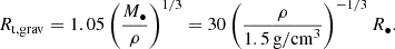
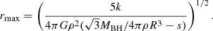
This is called the tidal downsizing process, which generates numerous small bodies. Figure 1 shows the maximum size a small body can survive as a function of the pericenter distance, for different cohesion strengths σc.
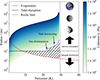 |
Fig. 1. Tidal downsizing and evaporation of planetary bodies. The maximum size of a planetary body surviving tidal forces is denoted by the gradient-filled regions; the color denotes the cohesive strength. The blue curve traces the maximum size of survivable small bodies under the tidal effect. Rubble piles (> 100 m) are typically assumed to have a cohesion of 1 Pa, whereas monolithic bodies (< 100 m) exhibit much higher cohesion, often exceeding 104 Pa. The vertical gray line marks the classical Roche limit. The red line represents the minimum size of survivable small bodies under evaporation via gas drag during a single flyby. The shaded region represents the parameter space where small bodies can persist against both tidal disruption and hydrodynamic ablation. |
By analogy with small Solar System bodies, the objects orbiting the SMBH are also rubble piles; they exhibit cohesive strengths of merely a few pascals. According to Sánchez & Scheeres (2014), the cohesive strength of Solar System rubble-pile small bodies is
 (6)
(6)
where rp is the particle size. For micron-sized surface particles, the cohesion can reach a few hundred pascals. Since the rubble piles (rp > 100 m) are made up of grains of a broad size range (e.g., from microns to meters or larger), estimates of real rubble-pile asteroids suggest cohesive strengths ranging from a few pascals to hundreds of pascals (Rozitis et al. 2014; Scheeres et al. 2010; Zhang et al. 2018). A structural analysis of Bennu, the target of NASA’s OSIRIS-REx mission, implies near-zero surface cohesion, as inferred from the forces measured during surface sampling operations (Walsh et al. 2022). Additionally, the low-speed mobilization of ejecta deposited near the crater suggests a cohesion of less than 2 Pa (Perry et al. 2022). The structure of the crater produced in the impact experiment on the asteroid Ryugu, the target of JAXA’s Hayabusa2, suggests σc ≥ 0.05 Pa (Jutzi et al. 2022). The low σc values of Bennu and Ryugu could be the result of their carbon-dominated compositions as both are classified as C-type asteroids based on the spectra. The S-type (silicate-dominated) asteroids may exhibit higher cohesive strengths. For example, the asteroid Didymos, the target of NASA’s DART mission, is estimated to have a cohesive strength ∼20 Pa (Zhang et al. 2021a; Agrusa et al. 2022). Since C-type asteroids are abundant and typically located closer to comets than S-type asteroids, we assume σ1c,rp ∼ 1 Pa for rubble-pile small bodies. As shown in Fig. 1, the large rubble piles (> 100 m) begin to fragment when crossing RRoche ∼ 30 R•. This downsizing process continues until their size is reduced to ∼100 m, where they become monolithic bodies with much higher material strength. The closest distance for rubble piles to survive is ∼18 R•.
For monolithic bodies, the dependence of material strengths on size is still uncertain. Based on the observed meteoroids, the material strength can be described by
 (7)
(7)
Here α could vary from 0.05 to 0.5 (Popova et al. 2011). We assume α ∼ 0.2. An analysis of the size and depth of craters observed on boulders on the asteroid (101955) Bennu suggests σc, mn ∼ 0.44 − 1.70 MPa for meter-sized boulders (Ballouz et al. 2020). The boulders on the asteroid Ryugu suggest a lower strength 0.2–0.28 MPa (Grott et al. 2019). Constraints by the spin limit of asteroids (Zhang & Michel 2021) give σ0 = 10 kPa, r0 = 0.5 km, and α = 1/6. Despite the considerable uncertainty associated with material strength, various estimation methods consistently indicate that the material strength is higher than > 10 kPa for small bodies with radii smaller than 100 m. Therefore, these monolithic objects can reach the vicinity of the black hole (e.g., ≪18 R•).
2.2. Disintegration caused by gas pressure
However, the gas pressure can disintegrate the object if the gas pressure exceeds the object’s bounding strength. Assuming disk accretion, the gas density ρg at a distance R is
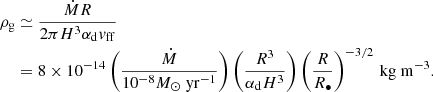 (8)
(8)
Here 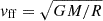 is the free-fall velocity. The scaled height of the disk near the black hole, H/R, can be approximated as 1 (Narayan et al. 1998). The viscosity parameter αd generally remains constant for magnetically arrested disks, while it decreases with distance for the weakly magnetized flow (Liska et al. 2020; Chatterjee & Narayan 2022). A recent general relativistic magnetohydrodynamic simulation on Sgr A★ suggests a constant αd (Chatterjee et al. 2023). Here we adopted αd ∼ 0.3, as suggested by Narayan et al. (1998). The parameter Ṁ is the accretion rate. Observations of Faraday rotation in polarized millimeter emissions suggest a range between 10−7 and 10−9 solar masses per year (Bower et al. 2003; Marrone et al. 2006). Further support comes from the Event Horizon Telescope (EHT) (Akiyama et al. 2022). Modeling suggests that the accretion rate near the event horizon is less than 10−8 M⊙ yr−1. For this work we used Ṁ ∼ 10−8 M⊙ yr−1 for the vicinity of the black hole.
The ram pressure can be estimated as
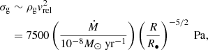 (9)
(9)
where ρg is the gas density and 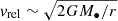 is the relative speed of an asteroid in a nearly parabolic orbit with respect to the gas disk.
For rubble-pile bodies, the survival condition is σg < σc, rb, which gives
 (10)
(10)
This distance is slightly larger than the tidal disruption distance for rubble piles, indicating that rubble piles should become disrupted due to tides around ∼22R•, within which small bodies can only exist in the form of monolithic objects. On the other hand, monolithic objects can easily survive from the gas pressure as their strength (e.g., > 10 kPa) is much greater than σg.
3. Evaporation and erosion of fragments
We show that large objects can survive down to 22R•, where they fragment into smaller bodies with sizes below 100 m as a result of gas pressure and tides. However, these small objects may undergo evaporation during a flyby due to frictional heating by the surrounding gas. In this section, based on the fireball model, we estimate the closest distances these small fragments can approach without being completely evaporated during a single passage, and we evaluate the resulting luminosity.
3.1. Evaporation
The aerodynamic friction experienced by a planetary object moving through the surrounding gas leads to surface heating and potential evaporation. We follow the approach of Zubovas et al. (2012) to estimate the evaporation rate. The mass-loss rate can be estimated by using the classical meteor ablation formula (Bronshten 1983):
 (11)
(11)
Here CH ∼ 1 is a dimensionless factor that measures the fraction of the energy that is used for evaporation instead of thermal emission (Zubovas et al. 2012). The parameter Q ∼ 3 × 10⁶ J kg−1 is the specific heat of ablation, which is the energy required to ablate a unit mass of the material (Borovička et al. 2007). The radius shrinkage rate is
 (12)
(12)
Here we assume the density ρ ∼ 3000 kg m−3, which is the typical grain density of carbonaceous chondrite meteorites (Flynn et al. 1999). After the time spent by the object at a distance comparable to the pericenter radius,  , the evaporation radius is
  m.
m.
The red curve in Fig. 1 represents the depth of evaporation caused by frictional heating during a single pericenter passage, setting a lower limit on the size of surviving objects. This analysis suggests that the largest monolithic objects can reach ∼8R•. This location is consistent with the flare observed at ∼7R• (Vincent et al. 2011; GRAVITY Collaboration 2023).
These estimates assume that objects experience continuous gas friction throughout a flyby and that their velocity is not significantly reduced by gas drag. Below, we justify these assumptions. Objects with inclination sin i < H/R are embedded in the gas disk and continuously experience drag heating. Objects with sin i > H/R experience a heating time ∼tflyH/πR. However, considering the value of H/R ∼ 1 in the vicinity of the black hole, the objects that come from the stellar disk with i < 45° are expected to be embedded in the gas disk, and thus subject to sustained heating. If the aerodynamic drag slows the fragments on a timescale shorter than the evaporation timescale, the fragments will co-move with the ambient gas, effectively halting further evaporation. However, in Appendix A, we show that the aerodynamic stopping time is much longer than the evaporation time.
3.2. Discussions on luminosity
The interaction between evaporated small-body fragments and the background accretion flow could generate strong emissions through different mechanisms, including high-energy electrons generated after sublimation and the thermal emission. Through high-energy electrons, Zubovas et al. (2012) assumed that the power released by a fragment is a fraction of the rest-mass energy per unit time, i.e.,
 (13)
(13)
Here ξ ∼ 0.1 is the dimensionless fraction of the released rest-mass energy (Zubovas et al. 2012). The pericenters of the fragments of the parent planetary scatter randomly around the disk and can be evaporated during one or a few passages to the black hole. The total bulk energy of the fragments is equal to that of the parent body. For a 10 km object, the luminosity could reach 3 × 1035 erg s−1.
Here we reinvestigate the scenario of thermal emission of fragments by adopting the fireball flare model. As the fragments spread out, each fragment heats up individually, increasing the total surface area exposed to the atmosphere (see, e.g., Fig. 5 in Hulfeld et al. (2021)). This could result in a sudden burst of light or flare as the fragments continue to ablate, releasing energy over a short time. A similar mechanism is responsible for the bright flashes observed during meteor fireballs in Earth’s atmosphere.
Simulations by Hulfeld et al. (2021) indicate that shortly after fragment formation, there is no mutual shielding among fragments, meaning that each fragment grain receives the full heat flux without obstruction. A commonly used approach to estimate the luminosity of each fragment is
 (14)
(14)
where f is the luminosity efficiency and ṙ can be obtained from Eq. (12).
To determine the total luminosity produced by all fragments, an appropriate size distribution must be adopted. We implement the size distribution of meteor fragments, which has been studied extensively based on recovered meteoritic debris. Several distribution models have been considered in previous works, including a simple power law (Frost 1969), a power law with an exponential cutoff (Oddershede et al. 1998; Vinnikov et al. 2016; Gritsevich et al. 2017), a third-degree polynomial (Badyukov & Dudorov 2013), and bimodal distributions. Recent findings by Brykina & Egorova (2024) indicate that the mass distribution of meteorite fragments and impact experiment debris is well described by a power law of the form dN ∝ m−βdm, which could translate to a size distribution of
 (15)
(15)
Applying the condition that the total mass of fragments equals the mass of the parent body, we have
 (16)
(16)
where r0 is the size of the parent body, and rmin and rmax are the minimum and maximum size of the fragments. The total luminosity can be calculated by summing up the energy released by all the fragments,
 (17)
(17)
which gives the relation between the parent body size, r0, and the total luminosity, Lfireball. In our calculation, we take rmin = 100 μm, as suggested by observations of meteors (Borovička et al. 2007), and rmax= 100 m. The power index, β, is found to be ∼1.45–1.7 for meteoritic fragments and ∼1.68–1.88 for impact experiment fragments (Brykina & Egorova 2024). They also found there could be bias against small fragments in the collection, suggesting that the β could become larger when more fragments are collected. Fragments produced via tidal disruption follow a different size distribution.
Numerical simulations by Zhang & Lin (2020) demonstrate that the size distribution of tidal fragments cannot be described by a single power law. For large fragments with sizes exceeding 30% of the parent body’s radius, the power-law index is as steep as β ∼ 3, while for smaller fragments β is ∼1.3. This shallower distribution may result from the re-union of the fragments due to the self-gravity in the gas-free environment, which is not suitable when accounting for the disruption process induced by the gas flow around the black hole. Therefore, we implement the size distribution of meteor fragments instead of tidal fragments. We chose β = 1.8 for this study.
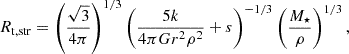
Figure 2 shows the luminosity generated by asteroids based on the two mechanisms discussed above. Our calculation indicates that the fireball luminosity produced by a parent body with radius r = 10 km could reach 5 × 1036 erg/s at 8R•, typically one order of magnitude higher than the bulk energy luminosity. As illustrated in Fig. 2, planetary bodies with radii from a few kilometers to ten kilometers are sufficient to reproduce the observed flare luminosities. In contrast to Zubovas et al. (2012), we show that the thermal emission from fragments could reproduce the observed luminosity using the fireball model adopted in meteor luminosity studies. However, it is likely that multiple emission mechanisms contribute to the observed flares. Our estimated size requirement is slightly smaller than their 10 km estimate.
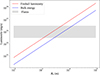 |
Fig. 2. Luminosity produced by asteroids at ∼8 R• based on the estimate of the bulk energy (red) and the fireball luminosity (blue). The luminosity of the observed flares is represented by the gray region. |
While the exact emission mechanism remains uncertain, we can compare the statistical properties of observed flares with those expected from asteroid-induced emissions. The flare frequency–luminosity relation is described by dNf ∝ L−αL. Statistical studies suggest αL to be 1.9 (Neilsen et al. 2013), 1.8 (Wang et al. 2015), 1.65 (Li et al. 2015), and 1.73 (Yuan et al. 2018). For asteroid-induced flares, luminosity is proportional to mass. Under a collisional cascade, the asteroid mass distribution follows a power law with index 1.83, implying αL = 1.83, consistent with the observational range.
The duration distribution of flares does not follow a clear power law (Yuan et al. 2018), but may be approximated by tf ∝ L−αt with αt < 0.55 (Li et al. 2015). In the asteroid emission scenario, the flare duration corresponds to the evaporation time, tevap = r/ṙ. Since ṙ is independent of r (Eq. 12), we find tf ∝ r ∝ m−1/3 ∝ L−1/3, consistent with constraint of αt < 0.55.
4. Delivery of planetary bodies to Sgr A★
Sgr A★ is surrounded by a nuclear cluster of N★ ∼ M•/M★ old stars (Schödel et al. 2007; Trippe et al. 2008) with solar or subsolar masses M★. Under the dominance of the SMBH’s gravity, these stars undergo scalar resonant relaxation (Rauch & Tremaine 1996; Hopman & Alexander 2006; Yu et al. 2007), which redistributes angular momentum among themselves. On a secular (scalar relaxation) timescale τsecular ∼ P★M•/M★(∼109 yr at 0.1pc), a small fraction of stars attain a sufficiently small pericenter distance Rperi(≲Rt, grav, Eq. (1)) to undergo tidal disruption (Rees 1988). Under the assumption that the cluster’s dynamical structure evolved concurrently with the growth of the SMBH’s mass, M•, the stellar tidal disruption rate around Sgr A★ is expected to be ∼10−5 yr−1 (Alexander 2005). Since close-in super-Earths are common around solar-type stars (Kunimoto & Matthews 2020; Bryson et al. 2021), they may accompany their host stars destined to the SMBH proximity at a rate of ∼10−11 M⊙ yr−1, corresponding to a rest-mass energy flux of a few × 1035 erg s−1, sufficient to account for the observed flare energetics.
Host stars cannot retain planets or small bodies with a semimajor axis asb ≳ Rperi(M★/M•)1/3. For the main belt-like asteroids and Kuiper belt-like objects, the detachment distance is Rperi ∼ 400 AU > > Rt,grav and ∼ 7000 AU, respectively. For super-Earths with periods that range from weeks to months, the detachment distance is Rperi∼ a few AU, well outside Rt, grav. After their detachment from their host stars, resonant relaxation leads some freely floating planetary bodies, including small bodies and gas giants, to Rt, grav for tidal disruption of their gaseous envelopes and to Rt, str (Eq. 2) for tidal downsizing of their solid cores. Zubovas et al. (2012) reproduced the delivery rate inferred from the observed outbursts under the assumption that all the cluster stars carry a population of Nsb outlying (beyond the ice giant planets) small bodies with a total mass Mtotal ∼ 10−5 M⊙. Their time-average detachment rate is ∼N★Nsb/τsecular. The assumed magnitude of Mtotal is comparable to that of super-Earths and long-period Neptune-mass planets (Zang et al. 2025). It is a fraction that of the primordial Kuiper belt required (∼6 × 10⁻⁵ M⊙) to establish the current kinematic structure of the outer Solar System (Gomes et al. 2005; Nesvorný et al. 2018). Comparable masses have been inferred for debris disks around other main sequence stars, including β Pictoris. It is also within the range needed to continually pollute the atmospheres of some white dwarfs (Zhang et al. 2021b).
Although concurrent mass segregation is associated with dynamical friction (also leading to a gradual depletion of freely floating small bodies and planets from the nuclear cluster), it proceeds on a characteristic timescale of τloss = 109 yr, which is ∼τsecular. In a continuous detachment-loss equilibrium, the population of small bodies in the nuclear cluster remains relatively constant over time.
Here we consider another potential supply that increases the tidal disruption rates of stars and planetary bodies. Sgr A★ is surrounded by a group of young S stars (Ghez et al. 2003; Gillessen et al. 2017) with highly eccentric and isotropic orbits at 5 × 10⁻³ − 0.04pc, a clockwise rotating disk of O/WR stars (CWSs) with modest orbital eccentricities, and some off-the-disk B stars (ODSs) with high eccentricity and inclination (relative to the clockwise-rotating disk) extends from approximately 0.04 pc to 0.5 pc (Levin & Beloborodov 2003; Paumard et al. 2006; Lu et al. 2009; Yelda et al. 2014; Ali et al. 2020; von Fellenberg et al. 2022). These young massive stars (∼200 in number) either recently formed through gravitational instability(Goodman 2003) or rejuvenated after being captured (Artymowicz et al. 1993; Davies & Lin 2020) by a gaseous disk around the SMBH. These young stars are likely to be surrounded by their own protoplanetary disks, some of which may have persisted for several megayears and manifested as G-clouds (Gillessen et al. 2019; Owen & Lin 2023). The planet formation probability in these protoplanetary disks may be increased (Ida & Lin 2004) by the supersolar metallicity commonly found in typical active galactic nucleus (AGN) disks (Huang et al. 2023). Moreover, entities with masses comparable to planets, also known as blanets, may also form in situ and concurrently with emerging stars, directly within the disk around the SMBH (Wada et al. 2019, 2021).
Although the natal disk of S stars, CWSs, and ODEs no longer exists in the proximity of Sgr A★ today, its surface density and temperature distribution may be inferred from AGN disks around other SMBHs with similar M•. These quantities have been extrapolated from the reverberation mapping and radiation transfer models of broad emission lines and spectral energy distribution of typical AGN disks. The interaction of embedded and surrounding stars with their natal disk increases their in-spiral and tidal disruption rates (MacLeod & Lin 2020; Wang et al. 2024). During the depletion of their natal disk, the stars’ eccentricity e★ is further excited, together with a decline in their Rperi by either the von Zeipel-Lidov-Kozai effect (Valtonen & Karttunen 2006) or sweeping secular resonance (Zheng et al. 2020, 2021) of any intermediate-mass companion to the SMBH, such as IRS 13E (Krabbe et al. 1995).
In comparison with the old nuclear cluster stars, these young stars have higher masses (M★ ∼ 15 M⊙). With their periods of decades to centuries, S stars’ τsecular ∼ 107 yrs. Many (NS > 20) S stars also have Rperi ≲ 10−2 pc (Burkert et al. 2024). Around them, even planets with semimajor axes less than that of the ice giant planets in the Solar System and some known cold Jupiters around other stars in the solar neighborhood can also become detached from their hosts. These escapers form a super-Oort cloud composed of a population of planets and small bodies detached from their original host stars (Nayakshin et al. 2012). These free-floating planetary bodies provide a rich reservoir for subsequent planetary tidal disruption of their gaseous envelope and downsizing of their solid cores when they venture to the SMBH’s Rt, grav and Rt, str. Under the assumption that short-period super-Earths and long-period Neptunes are common (Kunimoto & Matthews 2020; Bryson et al. 2021; Zang et al. 2025), we estimate the total mass of the super-Oort cloud to be MSO ≳ NSM⊕ ∼ 1028 − 29 g. From these estimates, we infer a time-averaged delivery rate ∼MSO/τsecular ∼ 1013 − 15g s−1, which exceeds that needed to account for the flares.
5. Emission signatures from ionized asteroidal materials
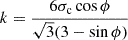
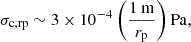
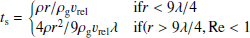
To investigate the observable spectral signatures of the post-flare under the asteroid disruption hypothesis, we computed photoionization models of the evaporated asteroidal gas using CLOUDY. We assumed that the fragments are exposed to the ionizing continuum associated with the observed flare SED of the Galactic center, scaled such that the incident ionizing flux at the cloud surface is ϕ = 2 × 10¹⁵ photons s−1 cm−2 (e.g., Fig.1 in Owen & Lin 2023). We assume that the composition of the gas reflects the supersolar metallicity expected for asteroid material, with Z = 100 Z⊙. The mean density of the evaporated material can be approximated as ρast = mast/vrelcs2tevp3. For a representative case with mast = 1019 g, vrel = 0.3c at 10 R•, cs ≤ 108 cm s−1, tevp = 30 min, we obtain ρast ∼ 1.5 × 10⁻¹⁷ g cm−3, which is equivalent to nH ≤ 107 cm−3. Four representative models are shown in Figure 3, corresponding to hydrogen densities nH = 106 and 107 cm−3 and total hydrogen column densities NH = 1016 and 1017 cm−2. A covering factor of C = 0.05 was adopted to account for the small projected area of the fragment swarm. In these models, the dominant emission features include C IVλ1550 and C IIIλ1909. For the higher-density and higher-column models, Fe II blend and [NeV] also become prominent.
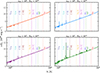 |
Fig. 3. Predicted UV–optical emission spectra of photoionized asteroid material irradiated by ionizing continuum with ϕ = 2 × 10¹⁵ photons s−1 cm−2. The four panels correspond to different combinations of gas density, nH = 106 (upper two panels) or 107 cm−3 (bottom) and total hydrogen column density, NH = 1018 (left) and 1019 cm−2 (right). Prominent emission lines are indicated by vertical dashed lines. We adopt a metallicity of Z = 100 Z⊙ and a covering factor of 5%. These spectra illustrate how the emission-line strengths vary with gas density and column depth in the evaporating asteroidal clouds. |
As shown in Figure 3, the emission-line luminosities systematically increase with gas density. We estimate the Strömgren radius ( ), RS = 2.3 × 10¹⁶ and 2.3 × 1014 cm for nH = 106 and 107 cm−3, respectively. The corresponding ionized columns are NS ≃ 2 × 10²² and 2 × 1021 cm−2, both far exceeding the adopted model columns implied by the size and density of the asteroidal material. This implies that the clouds are fully ionized in all cases, and therefore recombination lines are generally weak in the predicted spectra. Nevertheless, the higher-density models radiate more efficiently because the emissivity of collisionally excited lines scales approximately as
  , while the stronger cooling at high density lowers the equilibrium temperature (Te ∼ 104 K) and increases the efficiency of metal-line excitation. Consequently, intermediate ions such as C2+ and C3+ become more abundant, producing prominent CIII] and C IV features. The [Ne V] λ3426 line also becomes stronger with both higher density and larger column depth, since a larger column simply provides more emitting material within the fully ionized region. Together, these effects indicate that the enhanced C IV, CIII], and [Ne V] emission in the high-density model.
If we focus on the model that produces the strongest emission lines (nH = 107 cm−3 and NH = 1019 cm−2), the most prominent feature in the UV spectrum is the C IV line. The luminosities of individual lines are obtained by multiplying the CLOUDY surface flux by the illuminated surface area and the covering factor, yielding LC IV = 5.04 × 1027 erg s−1. This corresponds to an observed flux of 6.3 × 10⁻¹⁹ erg s−1 cm−2. For comparison, the 5σ line detection limit of HST/Cosmic Origins Spectrograph (COS Green et al. 2012) using the low-resolution grating G140L, which covers the C IV wavelength range, is approximately 10−15 erg s−1cm−2 for a typical total integration time of ∼1800 s (see, e.g., Anderson & Sunyaev 2016). Therefore, even the brightest predicted UV line would remain well below the current detection threshold.
In summary, the metal line emission has a characteristic luminosity of about 1029 to 1030 erg s−1, roughly five orders of magnitude lower than the typical emission from Sgr A★ (1035 to 1036 erg s−1). Consequently, any emission lines produced by vaporized asteroid material near the Galactic center would be far too faint to detect with the present-day instruments.
6. Summary and discussions
Sgr A★, the supermassive black hole at the center of the Milky Way, exhibits frequent short-duration flares across multiple wavelengths. The origin of these flares remains an open question. In this work, we revisited the mechanism involving the tidal disruption and subsequent evaporation of small planetary bodies. We refined the previous models by incorporating the material strengths constrained from recent space missions and dynamical studies.
We first analyzed the fragmentation of planetary bodies due to tidal forces and gas pressure. Large rubble-pile asteroids (> 100 m) with cohesion ∼1 Pa can survive down to ∼22R•, within which they break into monolithic fragments (< 100 m) of much higher material strength. These monolithic objects, possessing higher material strength, can withstand further tidal disruption, but may still be subject to evaporation via aerodynamic heating during their close passage around the black hole. We estimated the surface temperature and mass-loss rate of these fragments, demonstrating that the strongest monolithic bodies can survive as close as ∼8R• over one passage. This region is more consistent with observed locations (∼7R•) of flaring events than ∼20R• predicted by the previous study, which neglected material strength (Zubovas et al. 2012).
We examined the luminosity generated by small bodies and considered two emission mechanisms: (1) the bulk energy emission mechanism from high-energy electrons produced during sublimation, suggested by Zubovas et al. (2012), and (2) thermal emission modeled as fireball flares akin to meteor events in Earth’s atmosphere. In the fireball model, each fragment heats independently, releasing energy as surface area increases. Using a physically motivated fragment size distribution drawn from meteorite and impact studies, we integrated individual fragment luminosities to estimate the total emission. Our results show that a parent body of a few kilometers in size can produce fireball luminosities comparable to the flare luminosity.
Statistical comparisons with observed flares support the asteroid-induced flare hypothesis. The flare frequency–luminosity relation, expected to follow dN ∝ L−αL with αL ∼ 1.83, agrees with the observed values (αL ∼ 1.65 − 1.9; e.g., Neilsen et al. 2013; Wang et al. 2015; Li et al. 2015; Yuan et al. 2018). Additionally, the flare duration-luminosity scaling (tf ∝ L−αt) with αt ∼ 1/3, derived from fragment evaporation times aligns with observational constraints αt < 0.55 (Li et al. 2015). We found that the metal emission in the post-flare phase has a characteristic energy flux of νLν ∼ 1029 − 1030 erg s−1, five orders of magnitude lower than the emission of Sgr A★ (i.e., 1035 − 1036 erg s−1). Consequently, any emission lines produced by the vaporized asteroid material would be far too faint to be detected.
Finally, we consider the delivery of these kilometer-scale small bodies to the Roche limit of Sgr A★. These objects, originally from planetary systems around S stars, CWSs, ODSs, and nuclear cluster stars, are transported along with their host stars to Sgr A★’s proximity thanks to Sgr A★’s dominant gravity and stellar resonant relaxation. After their detachment from their host stars, their orbits continue to evolve through resonant relaxation. Free-floaters lose their gaseous envelope when their pericenter distance is reduce to ≲rt, grav. Eventually, their residual solid cores undergo tidal downsizing when their Rperi is reduced to rt, str. Assuming a total small-body mass comparable to that of the primordial Kuiper belt in the Solar System and the population of exoplanets, the delivery rate to the vicinity of the black hole could reach several per day, consistent with the frequency of observed flares.
Acknowledgments
We would like to thank Eiichiro Kokubo for the useful discussion. W.H. Zhou gratefully acknowledges the support and supervision received at the Observatoire de la Côte d’Azur, where the majority of this work was carried out. W.H.Zhou is currently affiliated with the University of Tokyo.
References
- Agrusa, H. F., Ferrari, F., Zhang, Y., Richardson, D. C., & Michel, P. 2022, Planet. Sci. J., 3, 158 [NASA ADS] [CrossRef] [Google Scholar]
- Akiyama, K., Alberdi, A., Alef, W., et al. 2022, ApJ, 930, L16 [NASA ADS] [CrossRef] [Google Scholar]
- Alexander, T. 2005, Phys. Rep., 419, 65 [CrossRef] [Google Scholar]
- Ali, B., Paul, D., Eckart, A., et al. 2020, ApJ, 896, 100 [NASA ADS] [CrossRef] [Google Scholar]
- Anderson, M. E., & Sunyaev, R. 2016, MNRAS, 459, 2806 [Google Scholar]
- Artymowicz, P., Lin, D. N. C., & Wampler, E. J. 1993, ApJ, 409, 592 [NASA ADS] [CrossRef] [Google Scholar]
- Badyukov, D. D., & Dudorov, A. E. 2013, Geochem. Int., 51, 583 [Google Scholar]
- Baganoff, F. K., Bautz, M. W., Brandt, W. N., et al. 2001, Nature, 413, 45 [Google Scholar]
- Ballouz, R. L., Walsh, K. J., Barnouin, O. S., et al. 2020, Nature, 587, 205 [NASA ADS] [CrossRef] [Google Scholar]
- Borovička, J., Spurný, P., & Koten, P. 2007, A&A, 473, 661 [NASA ADS] [CrossRef] [EDP Sciences] [Google Scholar]
- Bower, G. C., Wright, M. C. H., Falcke, H., & Backer, D. C. 2003, ApJ, 588, 331 [Google Scholar]
- Bronshten, V. A. 1983, Physics of Meteoric Phenomena (Dordrecht: Springer) [Google Scholar]
- Brykina, I. G., & Egorova, L. A. 2024, Planet. Space Sci., 241, 105838 [Google Scholar]
- Bryson, S., Kunimoto, M., Kopparapu, R. K., et al. 2021, AJ, 161, 36 [NASA ADS] [CrossRef] [Google Scholar]
- Burkert, A., Gillessen, S., Lin, D. N. C., et al. 2024, ApJ, 962, 81 [NASA ADS] [CrossRef] [Google Scholar]
- Čadež, A., Calvani, M., & Kostić, U. 2008, A&A, 487, 527 [NASA ADS] [CrossRef] [EDP Sciences] [Google Scholar]
- Chatterjee, K., & Narayan, R. 2022, ApJ, 941, 30 [NASA ADS] [CrossRef] [Google Scholar]
- Chatterjee, K., Chael, A., Tiede, P., et al. 2023, Galaxies, 11, 38 [NASA ADS] [CrossRef] [Google Scholar]
- Chiang, E., & Youdin, A. 2010, Ann. Rev. Earth Planet. Sci., 38, 493 [Google Scholar]
- Davies, M. B., & Lin, D. N. C. 2020, MNRAS, 498, 3452 [Google Scholar]
- Dodds-Eden, K., Sharma, P., Quataert, E., et al. 2010, ApJ, 725, 450 [NASA ADS] [CrossRef] [Google Scholar]
- Flynn, G. J., Moore, L. B., & Klöck, W. 1999, Icarus, 142, 97 [Google Scholar]
- Frost, M. J. 1969, Meteoritics, 4, 217 [Google Scholar]
- Genzel, R., Eckart, A., Ott, T., & Eisenhauer, F. 1997, MNRAS, 291, 219 [NASA ADS] [CrossRef] [Google Scholar]
- Genzel, R., Schödel, R., Ott, T., et al. 2003, Nature, 425, 934 [NASA ADS] [CrossRef] [Google Scholar]
- Ghez, A. M., Klein, B. L., Morris, M., & Becklin, E. E. 1998, ApJ, 509, 678 [NASA ADS] [CrossRef] [Google Scholar]
- Ghez, A. M., Duchêne, G., Matthews, K., et al. 2003, ApJ, 586, L127 [Google Scholar]
- Gillessen, S., Plewa, P. M., Eisenhauer, F., et al. 2017, ApJ, 837, 30 [Google Scholar]
- Gillessen, S., Plewa, P. M., Widmann, F., et al. 2019, ApJ, 871, 126 [NASA ADS] [CrossRef] [Google Scholar]
- Gomes, R., Levison, H. F., Tsiganis, K., & Morbidelli, A. 2005, Nature, 435, 466 [Google Scholar]
- Goodman, J. 2003, MNRAS, 339, 937 [NASA ADS] [CrossRef] [Google Scholar]
- GRAVITY Collaboration 2023, A&A, 677, L10 [NASA ADS] [CrossRef] [EDP Sciences] [Google Scholar]
- Green, J. C., Froning, C. S., Osterman, S., et al. 2012, ApJ, 744, 60 [NASA ADS] [CrossRef] [Google Scholar]
- Gritsevich, M., Dmitriev, V., Vinnikov, V., et al. 2017, Astrophys. Space Sci. Proc., 46, 153 [Google Scholar]
- Grott, M., Knollenberg, J., Hamm, M., et al. 2019, Nat. Astron., 3, 971 [Google Scholar]
- Holsapple, K. A. 2007, Icarus, 187, 500 [NASA ADS] [CrossRef] [Google Scholar]
- Holsapple, K. A., & Michel, P. 2008, Icarus, 193, 283 [NASA ADS] [CrossRef] [Google Scholar]
- Hopman, C., & Alexander, T. 2006, ApJ, 645, 1152 [NASA ADS] [CrossRef] [Google Scholar]
- Huang, J., Lin, D. N. C., & Shields, G. 2023, MNRAS, 525, 5702 [NASA ADS] [CrossRef] [Google Scholar]
- Hulfeld, L., Küchlin, S., & Jenny, P. 2021, A&A, 650, A101 [NASA ADS] [CrossRef] [EDP Sciences] [Google Scholar]
- Ida, S., & Lin, D. N. C. 2004, ApJ, 616, 567 [NASA ADS] [CrossRef] [Google Scholar]
- Jutzi, M., Raducan, S. D., Zhang, Y., Michel, P., & Arakawa, M. 2022, Nat. Commun., 13, 7134 [Google Scholar]
- Kostić, U., Čadež, A., Calvani, M., & Gomboc, A. 2009, A&A, 496, 307 [NASA ADS] [CrossRef] [EDP Sciences] [Google Scholar]
- Krabbe, A., Genzel, R., Eckart, A., et al. 1995, ApJ, 447, L95 [NASA ADS] [CrossRef] [Google Scholar]
- Kunimoto, M., & Matthews, J. M. 2020, AJ, 159, 248 [NASA ADS] [CrossRef] [Google Scholar]
- Levin, Y., & Beloborodov, A. M. 2003, ApJ, 590, L33 [NASA ADS] [CrossRef] [Google Scholar]
- Li, Y.-P., Yuan, F., Yuan, Q., et al. 2015, ApJ, 810, 19 [Google Scholar]
- Liska, M., Tchekhovskoy, A., & Quataert, E. 2020, MNRAS, 494, 3656 [Google Scholar]
- Liu, S., & Melia, F. 2002, ApJ, 566, L77 [Google Scholar]
- Lu, J. R., Ghez, A. M., Hornstein, S. D., et al. 2009, ApJ, 690, 1463 [NASA ADS] [CrossRef] [Google Scholar]
- MacLeod, M., & Lin, D. N. C. 2020, ApJ, 889, 94 [NASA ADS] [CrossRef] [Google Scholar]
- Markoff, S., Falcke, H., Yuan, F., & Biermann, P. L. 2001, A&A, 379, L13 [NASA ADS] [CrossRef] [EDP Sciences] [Google Scholar]
- Marrone, D. P., Moran, J. M., Zhao, J.-H., & Rao, R. 2006, ApJ, 640, 308 [NASA ADS] [CrossRef] [Google Scholar]
- Narayan, R., Mahadevan, R., & Quataert, E. 1998, in Theory of Black Hole Accretion Disks, eds. M. A. Abramowicz, G. Björnsson, & J. E. Pringle, 148 [Google Scholar]
- Nayakshin, S., Sazonov, S., & Sunyaev, R. 2012, MNRAS, 419, 1238 [Google Scholar]
- Neilsen, J., Nowak, M. A., Gammie, C., et al. 2013, ApJ, 774, 42 [NASA ADS] [CrossRef] [Google Scholar]
- Nesvorný, D., Vokrouhlický, D., Bottke, W. F., & Levison, H. F. 2018, Nat. Astron., 2, 878 [Google Scholar]
- Nowak, M. A., Neilsen, J., Markoff, S. B., et al. 2012, ApJ, 759, 95 [NASA ADS] [CrossRef] [Google Scholar]
- Oddershede, L., Meibom, A., & Bohr, J. 1998, EPL (Europhys. Lett.), 43, 598 [Google Scholar]
- Owen, J. E., & Lin, D. N. C. 2023, MNRAS, 519, 397 [Google Scholar]
- Paumard, T., Genzel, R., Martins, F., et al. 2006, ApJ, 643, 1011 [NASA ADS] [CrossRef] [Google Scholar]
- Perry, M., Barnouin, O., Daly, R., et al. 2022, Nat. Geosci., 15, 447 [NASA ADS] [CrossRef] [Google Scholar]
- Ponti, G., George, E., Scaringi, S., et al. 2017, MNRAS, 468, 2447 [NASA ADS] [CrossRef] [Google Scholar]
- Popova, O., Borovička, J., Hartmann, W. K., et al. 2011, Meteor. Planet. Sci., 46, 1525 [NASA ADS] [CrossRef] [Google Scholar]
- Rauch, K. P., & Tremaine, S. 1996, New Astron., 1, 149 [NASA ADS] [CrossRef] [Google Scholar]
- Rees, M. J. 1988, Nature, 333, 523 [Google Scholar]
- Rozitis, B., Maclennan, E., & Emery, J. P. 2014, Nature, 512, 174 [CrossRef] [Google Scholar]
- Sánchez, P., & Scheeres, D. J. 2014, Meteor. Planet. Sci., 49, 788 [Google Scholar]
- Scheeres, D. J., Hartzell, C. M., Sánchez, P., & Swift, M. 2010, Icarus, 210, 968 [NASA ADS] [CrossRef] [Google Scholar]
- Schödel, R., Eckart, A., Alexander, T., et al. 2007, A&A, 469, 125 [NASA ADS] [CrossRef] [EDP Sciences] [Google Scholar]
- Sridhar, S., & Tremaine, S. 1992, Icarus, 95, 86 [NASA ADS] [CrossRef] [Google Scholar]
- Trippe, S., Gillessen, S., Gerhard, O. E., et al. 2008, A&A, 492, 419 [NASA ADS] [CrossRef] [EDP Sciences] [Google Scholar]
- Valtonen, M., & Karttunen, H. 2006, The Three-Body Problem (Cambridge University Press) [Google Scholar]
- Vincent, F. H., Paumard, T., Perrin, G., et al. 2011, MNRAS, 412, 2653 [Google Scholar]
- Vinnikov, V. V., Gritsevich, M. I., Kuznetsova, D. V., & Turchak, L. I. 2016, Phys. Doklady, 61, 305 [Google Scholar]
- von Fellenberg, S. D., Gillessen, S., Stadler, J., et al. 2022, ApJ, 932, L6 [NASA ADS] [CrossRef] [Google Scholar]
- von Fellenberg, S. D., Roychowdhury, T., Michail, J. M., et al. 2025, ApJ, 979, L20 [Google Scholar]
- Wada, K., Tsukamoto, Y., & Kokubo, E. 2019, ApJ, 886, 107 [Google Scholar]
- Wada, K., Tsukamoto, Y., & Kokubo, E. 2021, ApJ, 909, 96 [NASA ADS] [CrossRef] [Google Scholar]
- Walsh, K. J. 2018, ARA&A, 56, 593 [NASA ADS] [CrossRef] [Google Scholar]
- Walsh, K. J., Ballouz, R.-L., Jawin, E. R., et al. 2022, Sci. Adv., 8, eabm6229 [NASA ADS] [CrossRef] [Google Scholar]
- Wang, F. Y., Dai, Z. G., Yi, S. X., & Xi, S. Q. 2015, ApJS, 216, 8 [Google Scholar]
- Wang, Y., Lin, D. N. C., Zhang, B., & Zhu, Z. 2024, ApJ, 962, L7 [NASA ADS] [CrossRef] [Google Scholar]
- Yelda, S., Ghez, A. M., Lu, J. R., et al. 2014, ApJ, 783, 131 [Google Scholar]
- Yu, Q., Lu, Y., & Lin, D. N. C. 2007, ApJ, 666, 919 [Google Scholar]
- Yuan, Q., Wang, Q. D., Liu, S., & Wu, K. 2018, MNRAS, 473, 306 [Google Scholar]
- Yusef-Zadeh, F., Bushouse, H., Arendt, R. G., et al. 2025, ApJ, 980, L35 [Google Scholar]
- Zang, W., Jung, Y. K., Yee, J. C., et al. 2025, Science, 388, 400 [Google Scholar]
- Zhang, Y., & Lin, D. N. 2020, Nat. Astron., 4, 852 [NASA ADS] [CrossRef] [Google Scholar]
- Zhang, Y., & Michel, P. 2021, Astrodynamics, 5, 293 [NASA ADS] [CrossRef] [Google Scholar]
- Zhang, Y., Richardson, D. C., Barnouin, O. S., et al. 2018, ApJ, 857, 15 [Google Scholar]
- Zhang, Y., Michel, P., Richardson, D. C., et al. 2021a, Icarus, 362, 114433 [CrossRef] [Google Scholar]
- Zhang, Y., Liu, S.-F., & Lin, D. N. C. 2021b, ApJ, 915, 91 [NASA ADS] [CrossRef] [Google Scholar]
- Zhao, J.-H., Young, K. H., Herrnstein, R. M., et al. 2003, ApJ, 586, L29 [NASA ADS] [CrossRef] [Google Scholar]
- Zheng, X., Lin, D. N. C., & Mao, S. 2020, ApJ, 905, 169 [Google Scholar]
- Zheng, X., Lin, D. N. C., & Mao, S. 2021, ApJ, 914, 33 [Google Scholar]
- Zubovas, K., Nayakshin, S., & Markoff, S. 2012, MNRAS, 421, 1315 [NASA ADS] [CrossRef] [Google Scholar]
Appendix A: Aerodynamic stopping timescale
The aerodynamic stopping timescale for a fragment due to gas drag is
when their relative speed is faster than the sound speed (Chiang & Youdin 2010). Here Re=rvrel/λcg is the Reynolds number. The mean free path of the gas λ is roughly
 (A.1)
(A.1)
where mH = 1.67 × 10⁻²⁴ g is the mass of the hydrogen atom and σH ∼ 3 × 10⁻¹⁵ cm2 is the effective collisional cross section. The Epstein regime applies to planetary bodies, for which the stopping time can be estimated as
 (A.2)
(A.2)
It turns out that the stopping time is so long that fragments of all sizes evaporate before they are coupled with the ambient gas.
All Figures
|
Fig. 1. Tidal downsizing and evaporation of planetary bodies. The maximum size of a planetary body surviving tidal forces is denoted by the gradient-filled regions; the color denotes the cohesive strength. The blue curve traces the maximum size of survivable small bodies under the tidal effect. Rubble piles (> 100 m) are typically assumed to have a cohesion of 1 Pa, whereas monolithic bodies (< 100 m) exhibit much higher cohesion, often exceeding 104 Pa. The vertical gray line marks the classical Roche limit. The red line represents the minimum size of survivable small bodies under evaporation via gas drag during a single flyby. The shaded region represents the parameter space where small bodies can persist against both tidal disruption and hydrodynamic ablation. |
| In the text | |
|
Fig. 2. Luminosity produced by asteroids at ∼8 R• based on the estimate of the bulk energy (red) and the fireball luminosity (blue). The luminosity of the observed flares is represented by the gray region. |
| In the text | |
|
Fig. 3. Predicted UV–optical emission spectra of photoionized asteroid material irradiated by ionizing continuum with ϕ = 2 × 10¹⁵ photons s−1 cm−2. The four panels correspond to different combinations of gas density, nH = 106 (upper two panels) or 107 cm−3 (bottom) and total hydrogen column density, NH = 1018 (left) and 1019 cm−2 (right). Prominent emission lines are indicated by vertical dashed lines. We adopt a metallicity of Z = 100 Z⊙ and a covering factor of 5%. These spectra illustrate how the emission-line strengths vary with gas density and column depth in the evaporating asteroidal clouds. |
| In the text | |
Current usage metrics show cumulative count of Article Views (full-text article views including HTML views, PDF and ePub downloads, according to the available data) and Abstracts Views on Vision4Press platform.
Data correspond to usage on the plateform after 2015. The current usage metrics is available 48-96 hours after online publication and is updated daily on week days.
Initial download of the metrics may take a while.