| Issue |
A&A
Volume 705, January 2026
|
|
|---|---|---|
| Article Number | A158 | |
| Number of page(s) | 7 | |
| Section | Atomic, molecular, and nuclear data | |
| DOI | https://doi.org/10.1051/0004-6361/202555886 | |
| Published online | 16 January 2026 | |
Potential energy surface and low-temperature rate coefficients of cyano thioformaldehyde (HCSCN) by collision with helium (He)
1
Department of Earth and Environmental Science, University of Pennsylvania,
Philadelphia,
PA
19104,
USA
2
Center for Innovation and Entrepreneurship, Imam Mohammad Ibn Saud Islamic University (IMSIU),
Riyadh
11623,
Saudi Arabia
3
LSAMA, Department of Physics, Faculty of Sciences, Tunis El-Manar University,
1060
Tunis,
Tunisia
4
Department of Chemistry, University of Pennsylvania,
Philadelphia,
PA
19104,
USA
★ Corresponding author: This email address is being protected from spambots. You need JavaScript enabled to view it.
Received:
10
June
2025
Accepted:
17
October
2025
Abstract
Molecular collisional data are essential for accurately modeling molecular abundances and excitation in the interstellar medium (ISM), yet remain scarce for many sulfur-bearing species. In this work, we calculate collisional rate coefficients for the near-prolate asymmetric top molecule HCSCN in collision with helium. A highly accurate three-dimensional potential energy surface (PES) was constructed at the CCSD(T)-F12a/aug-cc-pVTZ level of theory. Utilizing this PES, we performed coupled state calculations of inelastic cross sections for rotational transitions between the first 71 rotational levels with energies below 20 cm−1 and collisional energies up to 500 cm−1, from which we derived collisional rate coefficients up to 100 K. The calculated PES is highly anisotropic, exhibiting numerous minima with the deepest value being 53 cm−1 at certain positions in and out of the HCSCN molecule plane. The collisional rates obtained for the b-type transitions are of the same magnitude as those of a-type transitions, with a slight inferiority. The rotational relaxation rate coefficients have a propensity rule that favors |ΔJ| = 1, |Δka| = |Δkc| = 0 for a-type transitions, while ΔJ = 0, |ΔKa| = |ΔKc| = 1 for b-type transitions. These data provide important insights into sulfur chemistry in the ISM and will aid in more accurate modeling of molecular abundances in environments such as TMC-1.
Key words: ISM: atoms / ISM: molecules
© The Authors 2026
 Open Access article, published by EDP Sciences, under the terms of the Creative Commons Attribution License (https://creativecommons.org/licenses/by/4.0), which permits unrestricted use, distribution, and reproduction in any medium, provided the original work is properly cited.
This article is published in open access under the Subscribe to Open model. This email address is being protected from spambots. You need JavaScript enabled to view it. to support open access publication.
1 Introduction
The observed depletion of sulfur in the interstellar medium (ISM) remains a puzzle and a major area of research due to discrepancies between expected elemental abundances and detected sulfur-bearing species (Agúndez et al. 2018; Laas & Caselli 2019; Shingledecker et al. 2020; Ruffle et al. 1999). In cold dark clouds such as Taurus molecular cloud 1 (TMC-1), sulfur is severely depleted from the gas phase, with only a small fraction of cosmic sulfur appearing in molecules. Nonetheless, more than a dozen sulfur-bearing carbon molecules (organosulfur species) have been identified. Classic examples include the diatomic CS (Fuente et al. 2019), which serves as a tracer of dense interstellar gas. Sulfur-bearing molecules, in general, offer valuable diagnostic tools for probing the physical conditions, chemical composition, and evolutionary stages of astronomical environments, owing to their sensitivity to local density, temperature, and ionization conditions (Gorai et al. 2024; Viti et al. 2004). In recent years, sensitive line surveys have expanded the number of observed species, such as NCS, HCCS, C5S, H2CCS, HC(S)CCH, and HC(S)CN (Cernicharo et al. 2021a,b). More recently, Remijan et al. detected the c-C3H2S from the GOTHAM survey (Remijan et al. 2025), which completes the HCSCCH and H2CCCS isomeric family (Cernicharo et al. 2021a,b). TMC-1 hosts a remarkably rich inventory of sulfur-bearing molecules. This diversity is unexpected given the severe depletion of sulfur in the gas phase, challenging current astro-chemical models to explain their formation pathways.
The detection of the organosulfur species provides important clues about the chemistry of sulfur. As a carbon-rich environment, TMC-1 likely fosters efficient pathways to form complex sulfur compounds, and the current chemical models struggle to reproduce the observed abundances. Such molecules are far more abundant than models predict, indicating that current networks underestimate the available atomic sulfur or lack key reaction pathways (Vidal et al. 2017). For instance, the HCSCN abundance relative to H2 is estimated to be 1.3 × 10⁻¹⁰, which is about four times as abundant as its oxygen analog, HCOCN (Remijan et al. 2008), contrary to expectations based on oxygen’s higher cosmic abundance (Cernicharo et al. 2021b). Similarly, the HNCS/HSCN observed ratio deviates strongly from the model expectation (Cernicharo et al. 2024). Such discrepancies indicate that the formation and destruction processes, the physical and chemical conditions, are still misunderstood.
Detecting a new interstellar molecule is only the first step toward understanding its role and abundance. To properly model its line intensities under non-local thermodynamic equilibrium (non-LTE) conditions, it is essential to compute collisional rate coefficients and rotational cross sections for collisions with the main gas constituents, such as He or H2. If such data are absent or unreliable, model predictions will suffer from significant uncertainties. For instance, Bop et al. (Bop et al. 2024) have demonstrated that collisional processes can significantly impact the interpretation of molecular line emissions. Additionally, in star-forming environments such as TMC-1, the HNCO emission has been shown to deviate from LTE. A non-LTE radiative transfer approach is therefore required to accurately interpret the line profiles, making reliable collisional rate coefficients essential (Hernández-Gómez et al. 2019). The detection of HCSCN in TMC-1 now demands collisional data for accurate modeling. In the absence of such data, analyses of HCSCN lines have assumed a low rotational temperature (of a few Kelvin). This LTE-like assumption is uncertain, especially if HCSCN’s levels are sub-thermally excited.
In this study, we present a novel three-dimensional (3D) potential energy surface (PES) for HCSCN-He, employing a highly accurate ab initio method. We calculated state-to-state rotational cross sections for HCSCN–He collisions using quantum scattering methods, and from these cross sections we derived temperature-dependent rate coefficients for a range of transitions. Such calculations are computationally demanding, as collisions involving asymmetric top molecules present a computational challenge due to the high density of rotational states arising from additional quantum numbers, Ka and Kc, in addition to J (Tebai et al. 2024). While collisions with H2 typically produce larger excitation cross sections and rate coefficients than with He, helium is often preferred due to its spherical geometry and computational simplicity. A scaling factor based on reduced mass can then be applied to estimate H2 collision rates from He-based data.
2 Potential energy surface
2.1 Methodology
In this study, HCSCN was treated as a planar rigid rotor by fixing its intramolecular bond lengths and angles at the calculated CCSD(T)-F12/aug-cc-pVTZ optimized equilibrium geometry (Trabelsi et al. 2025). Within this rigid rotor approximation, the PES for the HCSCN–He complex was defined in terms of Jacobi coordinates, as is illustrated in Figure 1. The OXYZ axes were chosen according to the principal axes of inertia of the HCSCN target molecule, i.e., X–>b, Y–>c, and Z–>a.
The R coordinate representing the distance between He and the HCSCN center of mass was varied from 4.0 to 50.0 Bohr. To capture short-range interactions more accurately, a finer grid of 0.2 Bohr steps was used in the range 4.0 ≤ R ≤ 12, followed by 12 to 16 in steps of 0.5 Bohr, while a coarser grid of 1.0 Bohr steps was employed for 16 < R ≤ 26. Additionally, five discrete R values (28, 30, 35, 40, and 50 Bohr) were included. The angular coordinate θ varied from 0° to 180° in increments of 5°, while ϕ was varied from 0° to 180° in steps of 10°. At each point on this grid, electronic energies were calculated within the C1 symmetry point group.
In total, the 3D PES of the HCSCN–He complex, V(R, θ, ϕ), was constructed using 64 × 19 × 37 = 44 992 energy points for distinct geometries. At each geometry, the basis set superposition error was corrected using the Boys and Bernardi procedure (Boys & Bernardi 1970),
![Mathematical equation: $\[V(R, \theta, \phi)=E_{\mathrm{HCSCN}-\mathrm{He}}(R, \theta, \phi)-E_{\mathrm{He}}(R, \theta, \phi)-E_{\mathrm{HCSCN}}(R, \theta, \phi),\]$](/articles/aa/full_html/2026/01/aa55886-25/aa55886-25-eq1.png) (1)
(1)
where EHCSCN(R, θ, ϕ), EHe(R, θ, ϕ), and EHCSCN–He(R, θ, ϕ) are the total electronic energies of HCSCN, He, and HCSCN–He, respectively. These energies were calculated with the full basis set of the HCSCN–He system. All calculations were done using MOLPRO software (Werner et al. 2012).
The T1 diagnostic (Lee 2003; Lee & Taylor 1989) for the weakly bound HCSCN–He system was found to be less than 0.02 for all calculated ab initio points, indicating a predominantly single-reference character and justifying the use of a coupled cluster approach. However, because the CCSD(T)-F12 method is not rigorously size-consistent (Knizia et al. 2009), the interaction energy does not vanish at infinite separation. Consequently, the residual interaction energy at a large distance (R = 50 Bohr) was subtracted for each orientation (θ, ϕ). It should be noted that the F12a variant was chosen as it typically recovers slightly more correlation energy than F12b.
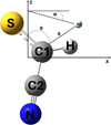 |
Fig. 1 Definition of the center of the Jacobi coordinates system (R, θ, ϕ) of the HCSCN–He complex. |
2.2 Results
In Figure 2, we present two-dimensional cuts of the HCSCN–He PES for He in the HCSCN plane corresponding to ϕ = {0, π} (panel a), in which Z = R cos(θ), X = R sin(θ), and Y = 0, and for He in the bisector plane corresponding to ϕ = π/2 (panel b), in which Z = R cos(θ), Y = R sin(θ), and X = 0. Panels c and d represent helium orbiting HCSCN in a spherical orbit of radius R = 6.2 Bohr and 7.4 Bohr, respectively.
Panel a of this figure reveals four minima on the PES in the molecular plane as helium approaches HCSCN. One minimum lies near the sulfur atom, with a depth of 30.47 cm−1 at R = 9.2 Bohr, θ = 25°, and ϕ = π. A second, deeper minimum (52.14 cm−1), is located near the hydrogen atom, 7 Bohr from the center of mass and inclined by 60° relative to the Z axis. The remaining two minima lie on either side of the carbon atom C2. The deeper one measures 53.03 cm−1 at θ = 125° and R = 7.4 Bohr, ϕ = 0, while the other is 38.36 cm−1 at R = 6.8 Bohr, θ = 105°, and ϕ = π. In the configuration in which helium is in a plane perpendicular to HCSCN (panel b), the PES displays a single minimum, corresponding to helium approaching from the C2 side at θ = 105° and R = 6.4 Bohr.
To analyze the anisotropy of the potential and to locate the minima, we have represented in panels c and d of Figure 4 sections of the equipotential when helium rotates on a spherical orbit around HCSCN. These cuts correspond to spherical orbits of the helium atom around the HCSCN molecule, at fixed radial distances of R = 6.2 Bohr (panel c) and R = 7.4 Bohr (panel d). In these representations, θ and ϕ define the orientation of helium with respect to the principal axes of the asymmetric top molecule HCSCN in spherical coordinates.
Panel d confirms the position of the deepest well observed in panel a, which has a depth of 53.30 cm−1 at the position θ = 122° and ϕ = 20°. Panel c shows us the existence of a well outside the plane of the molecule and the perpendicular one. This well is found at a slightly greater depth than the one in the plane, with a value of 53.76 cm−1. This global well is placed on the sphere of radius R = 6.2 Bohr, placed in the direction given by θ = 102° and ϕ = 112°.
Finally, to interpret the topographical features of the calculated PES, we performed natural bond orbital calculations using the M062X (Zhao & Truhlar 2008) in conjunction with the 6-311++G** basis set. The primary objective was to determine the atomic charge distribution, and the results of these calculations are presented in Table 1.
Close examination of Table 1 reveals that when the He atom nears the partial positive charges on the C2, H, and S atoms, its electron cloud is drawn to these positively charged sites. This attraction manifests as energy wells, which reflect the corresponding attractive potential in the PES. The partial positive charges on the C2, H, and S atoms are nearly identical (approximately +0.2). However, the large electron cloud around sulfur exerts additional repulsion on helium, resulting in a slightly shallower potential well on the sulfur side. The shallow well near S reflects a strong dispersion attraction to its polarizable electron cloud offset by moderate exchange repulsion. Conversely, the well near H is shifted away from the C–H axis due to significant exchange repulsion near the compact H atom. For the cut perpendicular to the plane of the molecule that has a single well, this can be explained by the fact that the H and S atoms containing (+) charges are outside this plane and that the only well at θ = 105° the single well aligns with C2 due to favorable dispersion to its region and reduced repulsion compared to S/H sites.
Panel c of Figure 2 confirms the position of the global minimum when He approaches HCSCN for θ = 102° and ϕ = 112°; this position corresponds exactly to He opposite the C2 carbon of HCSCN, forming a quasi-bond with C2. The C2–He quasi-bond is perpendicular to the plane of HCSCN, of length approximately 5.2 Bohr. Though natural population analysis charges are similar for H, C2, and S (Table 1), the PES topology is governed by their differing polarizabilities and electron density distributions.
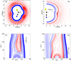 |
Fig. 2 Two-dimensional contour plots of the HCSCN–He PES. (a) Helium in the molecular plane; (b) in the bisector plane; (c) and (d) correspond to R = 6.2 and R = 7.4 Bohr, respectively. Red contours are attractive; blue contours are repulsive. |
Calculated net charge by natural population analysis for HCSCN molecule.
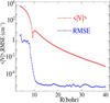 |
Fig. 3 Absolute value of the average interaction potential and the RMSE between the fit and ab initio calculated potential as a function of the separation distance, R. |
2.3 Analytical fit
To be introduced in the cross-section calculation, the 3D PES of HCSCN in interaction with helium was developed as follows:
![Mathematical equation: $\[V(R, \theta, \phi)=\sum_{l=0}^{l_{\max }} \sum_{m=0}^{m_{\max }} \frac{V_{l m}(R)\left(Y_{l, m}(\theta, \phi)+(-1)^m Y_{l,-m}(\theta, \phi)\right)}{1+\delta_{m 0}},\]$](/articles/aa/full_html/2026/01/aa55886-25/aa55886-25-eq2.png) (2)
(2)
where Yl,m(θ, ϕ) are the normalized spherical harmonic functions, Vlm(R) are the radial dependence coefficients to be included in MOLSCAT (Hutson & Green 1994; Hutson & Le Sueur 2019) software, and δm0 is the Kronecker symbol. For each value of R, a least-squares procedure with quadrature was used to deduce the Vlm(R) coefficients. From 37 × 19 values of (θ, ϕ), the PES was adjusted by 260 terms, l ≤ 25 and m ≤ 12.
To examine the accuracy of our fit PES, we determined the root mean square error (RMSE) following the method described by (Alborzpour et al. 2016) using 703 points. The RMSE quantifies the deviation between the fit potential and the original ab initio data across the configuration space. In Figure 3, we present the RMSE as a function of the intermolecular separation, R, plotted alongside the absolute value of the average interaction potential for each R spanning from 4 to 40 Bohr.
This figure shows that in the short-range repulsive region (R < 6 Bohr), the RMSE remains below 5 cm−1, reflecting good agreement even where the potential rises steeply. As the distance increases and the interaction enters the attractive region, the RMSE drops sharply, reaching values as low as 10−5 cm−1 near R = 10 Bohr. This drop indicates a high-quality fit in the region most relevant to the collisional dynamics and bound-state properties. It should be noted that the oscillations visible in Figure 3 are on the order of 10−5 cm−1, while the average potential in that region exceeds 10−3 cm−1. This corresponds to a relative error of less than 1%. Therefore, although minor oscillations are present, they are microscopic and are effectively corrected by the fitting procedure. The Vlm(R) coefficients were extrapolated at short distances (R < 4 Bohr) and at large distances (R > 40 Bohr) automatically using the POTNL routine of MOLSCAT. The R-dependent Vlm(R) components are represented in Figure 4 for m ≤ l ≤ 2. Therefore, the present PES shows enough accuracy to be employed in quantum dynamical calculations over a broad range of temperatures up to 100 K.
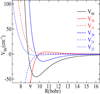 |
Fig. 4 Radial part of the interaction potential of the HCSCN–He molecular system for m ≤ l ≤ 2. |
3 Dynamical calculations
3.1 Rotational energy levels of HCSCN
HCSCN is a near-prolate asymmetric top-type molecule. The rotational Hamiltonian of such an asymmetric rotor is given by
![Mathematical equation: $\[H_{\mathrm{rot}}=A J_X^2+B J_Y^2+C J_Z^2-D_J J^4-D_{J K} J^2 J_Z^2-D_K J_Z^4,\]$](/articles/aa/full_html/2026/01/aa55886-25/aa55886-25-eq3.png) (3)
(3)
where A, B, and C represent the rotational constants, and DJ, DK, and DJK are the corresponding centrifugal distortion constants of HCSCN. The components JX, JY, and JZ denote the projections of the total rotational angular momentum, J, along the principal axes of the molecule, satisfying the relation ![Mathematical equation: $\[J^{2}= J_{X}^{2}+J_{Y}^{2}+J_{Z}^{2}\]$](/articles/aa/full_html/2026/01/aa55886-25/aa55886-25-eq4.png) . The rotational constants and centrifugal constants used in this study are in cm−1 and correspond to those measured by (Cernicharo et al. 2021b), i.e., A = 1.43132, B = 0.09907, C = 0.10659, DJ = 0.427 × 10⁻⁷, DJK = −0.340 × 10⁻⁵, and DK = 0.121 × 10⁻³.
. The rotational constants and centrifugal constants used in this study are in cm−1 and correspond to those measured by (Cernicharo et al. 2021b), i.e., A = 1.43132, B = 0.09907, C = 0.10659, DJ = 0.427 × 10⁻⁷, DJK = −0.340 × 10⁻⁵, and DK = 0.121 × 10⁻³.
For an asymmetric top molecule such as HCSCN, the rotational energy levels are typically labeled using the spectroscopic notation JKa Kc, where J is the rotational quantum number, and Ka and Kc are the projections of J onto the limiting prolate and oblate symmetric top axes, respectively. Figure 5 presents the energy diagram of the HCSCN molecule as a function of the Ka component for levels with energies below 100 cm−1. This figure shows a high density of HCSCN states, characterized by very small energy spacings between adjacent levels. This close spacing increases the number of energetically accessible open channels, which enhances the coupling between levels during collisions, leading to a higher probability of transitions between them.
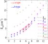 |
Fig. 5 HCSCN rotational levels up to 20 cm−1. Red and blue arrows indicate the a- and b-type observed transitions, respectively. |
Comparison of cross sections (Å2) calculated using CC and CS methods in molscat at different collision energies.
3.2 Cross section
Because HCSCN lacks identical nuclei that would give rise to ortho/para nuclear spin symmetries, all rotational levels contribute without symmetry based restrictions and must be treated simultaneously in the coupled-channel calculations. This requirement significantly increases the computational cost, rendering the close-coupling (CC) approach impractical. Instead, the coupled-states (CS) method, as implemented in MOLSCAT, was employed to compute collisional cross sections. To estimate the accuracy of CS results compared to CC results, we provided a test at three fixed energies: E=50, 100, and 200 cm−1. The results are presented in Table 2. This table shows that data provided by the CS method are very close to those given by the CC method, such that the relative error varies from 5 to 20%.
In our calculations, we included levels up to 13113 (corresponding to rotational energies up to Erot = 20 cm−1) and covered total energies from 0 to 500 cm−1. Several convergence tests were performed before proceeding with the cross-section calculations.
We examined the effect of the rotational basis size, defined by the maximum rotational quantum number Jmax, on the cross sections as a function of the total energy. Convergence was obtained with Jmax = 19 for E ≤ 100 cm−1 and Jmax = 22 for E> 100 cm−1. To better characterize the resonances in the cross section as a function of energy, we employed a fine energy grid at lower energies.
Specifically, for total energies below 50 cm−1, we used a step size of ΔE = 0.1 cm−1. The step size was then gradually increased to 0.2 cm−1 between E = 50 cm−1 and E = 100 cm−1, 1 cm−1 from 100 cm−1 to 200 cm−1, to 5 cm−1 until 300 cm−1, and finally to 10 cm−1 for 300 < E ≤ 500 cm−1.
In Figure 6, we present the variation in the inelastic cross sections ![Mathematical equation: $\[\sigma_{J_{K_{a} K_{c}} \rightarrow J_{K_{a}^{\prime} K_{c}^{\prime}}^{\prime}}\]$](/articles/aa/full_html/2026/01/aa55886-25/aa55886-25-eq5.png) (Ek) for the rotational excitation of HCSCN by He as a function of the collision energy, Ek. Panel a shows transitions from the rotational ground state, 000, to J0J levels (i.e., transitions with ΔJ = ΔKc and Ka = 0), while panel b focuses on transitions among the lowest sub-levels of J = 6, 7.
(Ek) for the rotational excitation of HCSCN by He as a function of the collision energy, Ek. Panel a shows transitions from the rotational ground state, 000, to J0J levels (i.e., transitions with ΔJ = ΔKc and Ka = 0), while panel b focuses on transitions among the lowest sub-levels of J = 6, 7.
The figure shows a structure of resonance features in the energy range Ek ≤ 50 cm−1, which corresponds closely to the depth of the potential well in the HCSCN–He interaction potential. These features include shape and Feshbach resonances. The latter likely arise from the formation of quasi-bound states, where the helium atom becomes temporarily trapped in the potential well of HCSCN before eventually dissociating.
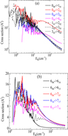 |
Fig. 6 Kinetic energy variation of rotating cross sections of HCSCN in collision with He for transitions from the ground state to J0J levels and for ΔJ = ΔKc with Ka = 0 (panel a) and between the J = 6, 7 lowest sub-levels (panel b). |
3.3 Rate coefficients
From the integration of the coupled-state calculated rotational cross sections, ![Mathematical equation: $\[\sigma_{J_{K_{a} K_{c}} \rightarrow J_{K_{a}^{\prime} K_{c}^{\prime}}^{\prime}}\]$](/articles/aa/full_html/2026/01/aa55886-25/aa55886-25-eq6.png) (Ek), over a Maxwell–Boltzmann distribution of velocities (i.e., kinetic energies) at a given temperature, T, the thermal rate coefficients,
(Ek), over a Maxwell–Boltzmann distribution of velocities (i.e., kinetic energies) at a given temperature, T, the thermal rate coefficients, ![Mathematical equation: $\[\sigma_{J_{K_{a} K_{c}} \rightarrow J_{K_{a}^{\prime} K_{c}^{\prime}}^{\prime}}\]$](/articles/aa/full_html/2026/01/aa55886-25/aa55886-25-eq7.png) (T), are expressed by
(T), are expressed by
![Mathematical equation: $\[k_{J_{K_a K_c} \rightarrow J_{K_a^{\prime} K_c^{\prime}}^{\prime}}(T)=\left(\frac{8}{\pi \mu k_B^3 T^3}\right)^{1 / 2} \int_0^{\infty} E_k \sigma_{J_{K_a K_c} \rightarrow J_{K_a^{\prime} K_c^{\prime}}^{\prime}}\left(E_k\right) e^{-E_k /\left(k_B T\right)} d E_k,\]$](/articles/aa/full_html/2026/01/aa55886-25/aa55886-25-eq8.png) (4)
(4)
where kB is the Boltzmann constant, T is the kinetic temperature, and μ = 3.786945 a.u. is the reduced mass of the HCSCN–He system. The variable Ek represents the relative kinetic energy between the colliding partners, and it is related to the total collisional energy by E = Ek + Erot, where Erot is the rotational energy of the initial state, JKaKc.
Figure 7 displays the temperature dependence of the rotational rate coefficients for HCSCN in collision with He, highlighting representative de-excitation pathways. In panel a, we show the a-type transitions from the lowest sub-level of each rotational state, J, labeled J0J down to the ground state (000) in solid lines, and to the corresponding lowest sub-level of the preceding rotational state (J − 1)0(J−1), i.e., ΔJ = ΔKc = −1 with Ka = 0, given in dashed lines. Panel b presents the b-type transitions within the same J manifold, specifically from Ka = 1 to Ka = 0, which involve a change in the angular momentum projection without a change in total J. More broadly, this figure shows that these rate coefficients exhibit a clear temperature dependence, influenced by the magnitude of the energy gap, the character of the rotational transition (a-type vs. b-type), and the anisotropy of the interaction potential.
In panel a, the two lowest rotational transitions, 101 → 000 and 202 → 000, dominate at different temperature regimes. The 101 → 000 is the most significant at temperatures below approximately 12 K, while the 202 → 000 becomes dominant at higher temperatures. This behavior was observed in previous work for Z-PGIM de-excitation by collision with He, when the 202 → 000 transition dominates the 101 → 000 for T > 10 K (Tebai et al. 2024). Furthermore, the rate coefficients for other transitions generally decrease as the rotational quantum number difference, ΔJ, increases, consistent with the lower probability of populating higher-lying states via inelastic collisions.
In panel b, the rate coefficients of the transitions between the lowest rotational levels decrease considerably with temperature. This phenomenon has been observed for the H2CO system in collision with H2 (Troscompt et al. 2009).
In panel c, the b-type transitions are presented, characterized by selection rules ΔJ = 0, ΔKa = −1, and ΔKc = 0 or 1. At low temperatures, the rate coefficients for all these transitions are closely clustered around 2 × 10⁻¹¹ cm3 s−1, having a slightly decreasing appearance as a function of T. From T = 10 K, the transitions with ΔKc = 1 exhibit a slow increase in their rate coefficients, while remaining on the order of 2 × 10⁻¹¹ cm3 s−1. In contrast, transitions with ΔKc = 0 show a more pronounced decline, reaching values of around 10−12 cm3 s−1 at higher temperatures. An additional observation from this panel is that, for transitions with ΔKc = 1, the rate coefficients tend to increase with the total rotational quantum number, J, indicating a higher probability of such transitions in more excited states. This trend is not observed for transitions with ΔKc = 0; for instance, the 918 → 909 transition exhibits one of the lowest rate coefficients among the set.
In panel c, we present the rate coefficients for a-type transitions characterized by ΔJ = −1. Similar to panel b, all transitions begin with rate coefficients around 2 × 10⁻¹¹ cm3 s−1 at low temperature. Around 10 K, transitions with ΔKa = ΔKc = 0 begin to diverge from the others, showing a steady increase with temperature and reaching values of approximately 5 × 10⁻¹¹ cm3 s−1 at higher temperatures.
In contrast, most of the remaining transitions exhibit a mild decrease with temperature, except for a few – namely, 212 → 111, 312 → 211, and 211 → 110 – that display a slight increase up to 25 K before gradually decreasing. Additionally, panel c shows that for transitions with ΔJ = −1 and ΔKa = ΔKc = 0, the rate coefficients tend to increase with increasing J, indicating enhanced transition probabilities at higher rotational levels. Conversely, for transitions defined by ΔJ = ΔKc = −1, ΔKa = 0, the rates show some crossing behavior at intermediate J values but eventually follow a decreasing trend beyond 25 K.
From these observations, it is evident that the collisional rate coefficients for b-type transitions in the HCSCN–He system are generally on the same order of magnitude as those for a-type transitions, albeit slightly lower on average. Regarding the dominant transition pathways, we can conclude that for a-type transitions, those characterized by ΔJ = −1, ΔKa = ΔKc = 0 are the most significant. In contrast, for b-type transitions, the most prominent are those with ΔJ = 0, |ΔKa| = |ΔKc| = 1, indicating a strong propensity for transitions involving simultaneous changes in the rotational angular momentum projections while conserving the total J.
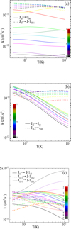 |
Fig. 7 Temperature variation of rotational rate coefficients (k) of HCSCN in collision with He, for a- and b-type transitions in panels a and b, respectively, and for ΔJ = −1, ΔKa = 0 and ΔKc = 0, −1 (a- and b-type) in panel c. |
4 Conclusions
For accurate ISM molecular abundance derivation, collisional rate coefficients at various temperatures are needed. In this work, we constructed a high-quality 3D PES at the CCSD(T)-F12/aug-cc-pVTZ level of theory, revealing four distinct potential wells, with the deepest reaching 53.76 cm−1. We then calculated cross sections for collision energies up to 500 cm−1, from which rate coefficients for temperatures up to 100 K were determined.
The b-type and a-type collisional rates are similar in magnitude, though b-type rates are marginally lower. This new data will be valuable for improving estimates of HCSCN abundances in astrophysical environments and advancing our understanding of sulfur chemistry in the ISM, especially in the Taurus Molecular Cloud (TMC-1). The rate coefficients presented here provide the essential input data for future radiative transfer modeling of HCSCN emission lines.
Data availability
The HCSCN-He rate coefficients are available on the BASECOL database (Dubernet et al. 2024).
Acknowledgements
This work was supported and funded by the Deanship of Scientific Research at Imam Mohammad Ibn Saud Islamic University (IMSIU) (grant number IMSIU-DDRSP2502).
References
- Agúndez, M., Marcelino, N., Cernicharo, J., & Tafalla, M. 2018, A&A, 611, L1 [NASA ADS] [CrossRef] [EDP Sciences] [Google Scholar]
- Alborzpour, J. P., Tew, D. P., & Habershon, S. 2016, J. Chem. Phys., 145, 174112 [Google Scholar]
- Bop, C. T., Agúndez, M., Cernicharo, J., Lefloch, B., & Lique, F. 2024, A&A, 681, L19 [NASA ADS] [CrossRef] [EDP Sciences] [Google Scholar]
- Boys, S. F., & Bernardi, F. 1970, Mol. Phys., 19, 553 [NASA ADS] [CrossRef] [Google Scholar]
- Cernicharo, J., Cabezas, C., Agúndez, M., et al. 2021a, A&A, 648, L3 [EDP Sciences] [Google Scholar]
- Cernicharo, J., Cabezas, C., Endo, Y., et al. 2021b, A&A, 650, L14 [NASA ADS] [CrossRef] [EDP Sciences] [Google Scholar]
- Cernicharo, J., Agúndez, M., Cabezas, C., et al. 2024, A&A, 682, L4 [NASA ADS] [CrossRef] [EDP Sciences] [Google Scholar]
- Dubernet, M., Boursier, C., Denis-Alpizar, O., et al. 2024, A&A, 683, A40 [NASA ADS] [CrossRef] [EDP Sciences] [Google Scholar]
- Fuente, A., Navarro, D., Caselli, P., et al. 2019, A&A, 624, A105 [NASA ADS] [CrossRef] [EDP Sciences] [Google Scholar]
- Gorai, P., Law, C.-Y., Tan, J. C., et al. 2024, ApJ, 960, 127 [NASA ADS] [CrossRef] [Google Scholar]
- Hernández-Gómez, A., Sahnoun, E., Caux, E., et al. 2019, MNRAS, 483, 2014 [CrossRef] [Google Scholar]
- Hutson, J., & Green, S. 1994, Collaborative Computational Project, 6 [Google Scholar]
- Hutson, J. M., & Le Sueur, C. R. 2019, Comput. Phys. Commun., 241, 9 [NASA ADS] [CrossRef] [Google Scholar]
- Knizia, G., Adler, T. B., & Werner, H.-J. 2009, J. Chem. Phys., 130, 054104 [Google Scholar]
- Laas, J. C., & Caselli, P. 2019, A&A, 624, A108 [NASA ADS] [CrossRef] [EDP Sciences] [Google Scholar]
- Lee, T. J. 2003, Chem. Phys. Lett., 372, 362 [Google Scholar]
- Lee, T. J., & Taylor, P. R. 1989, Int. J. Quant. Chem., 36, 199 [Google Scholar]
- Remijan, A. J., Hollis, J., Lovas, F., et al. 2008, ApJ, 675, L85 [NASA ADS] [CrossRef] [Google Scholar]
- Remijan, A. J., Changala, P. B., Xue, C., et al. 2025, ApJ, 982, 191 [Google Scholar]
- Ruffle, D., Hartquist, T., Caselli, P., & Williams, D. 1999, MNRAS, 306, 691 [NASA ADS] [CrossRef] [Google Scholar]
- Shingledecker, C. N., Lamberts, T., Laas, J. C., et al. 2020, ApJ, 888, 52 [Google Scholar]
- Tebai, Y., Khalifa, M. B., Khadri, F., & Hammami, K. 2024, Phys. Chem. Chem. Phys., 26, 24901 [Google Scholar]
- Trabelsi, T., El-Tohamy, M. F., Mostafa, G. A., & Francisco, J. S. 2025, J. Chem. Phys., 162, 044307 [Google Scholar]
- Troscompt, N., Faure, A., Wiesenfeld, L., Ceccarelli, C., & Valiron, P. 2009, A&A, 493, 687 [NASA ADS] [CrossRef] [EDP Sciences] [Google Scholar]
- Vidal, T. H., Loison, J.-C., Jaziri, A. Y., et al. 2017, MNRAS, 469, 435 [NASA ADS] [CrossRef] [Google Scholar]
- Viti, S., Collings, M. P., Dever, J. W., McCoustra, M. R., & Williams, D. A. 2004, MNRAS, 354, 1141 [NASA ADS] [CrossRef] [Google Scholar]
- Werner, H.-J., Knowles, P. J., Knizia, G., et al. 2012, See http://www.molpro.net [Google Scholar]
- Zhao, Y., & Truhlar, D. G. 2008, Theor. Chem. Acc., 120, 215 [CrossRef] [Google Scholar]
All Tables
Comparison of cross sections (Å2) calculated using CC and CS methods in molscat at different collision energies.
All Figures
|
Fig. 1 Definition of the center of the Jacobi coordinates system (R, θ, ϕ) of the HCSCN–He complex. |
| In the text | |
|
Fig. 2 Two-dimensional contour plots of the HCSCN–He PES. (a) Helium in the molecular plane; (b) in the bisector plane; (c) and (d) correspond to R = 6.2 and R = 7.4 Bohr, respectively. Red contours are attractive; blue contours are repulsive. |
| In the text | |
|
Fig. 3 Absolute value of the average interaction potential and the RMSE between the fit and ab initio calculated potential as a function of the separation distance, R. |
| In the text | |
|
Fig. 4 Radial part of the interaction potential of the HCSCN–He molecular system for m ≤ l ≤ 2. |
| In the text | |
|
Fig. 5 HCSCN rotational levels up to 20 cm−1. Red and blue arrows indicate the a- and b-type observed transitions, respectively. |
| In the text | |
|
Fig. 6 Kinetic energy variation of rotating cross sections of HCSCN in collision with He for transitions from the ground state to J0J levels and for ΔJ = ΔKc with Ka = 0 (panel a) and between the J = 6, 7 lowest sub-levels (panel b). |
| In the text | |
|
Fig. 7 Temperature variation of rotational rate coefficients (k) of HCSCN in collision with He, for a- and b-type transitions in panels a and b, respectively, and for ΔJ = −1, ΔKa = 0 and ΔKc = 0, −1 (a- and b-type) in panel c. |
| In the text | |
Current usage metrics show cumulative count of Article Views (full-text article views including HTML views, PDF and ePub downloads, according to the available data) and Abstracts Views on Vision4Press platform.
Data correspond to usage on the plateform after 2015. The current usage metrics is available 48-96 hours after online publication and is updated daily on week days.
Initial download of the metrics may take a while.