| Issue |
A&A
Volume 705, January 2026
|
|
|---|---|---|
| Article Number | A4 | |
| Number of page(s) | 11 | |
| Section | Astrophysical processes | |
| DOI | https://doi.org/10.1051/0004-6361/202556161 | |
| Published online | 19 December 2025 | |
Line-force-driven wind from a thin disk in a tidal disruption event
1
Shanghai Key Lab for Astrophysics, Shanghai Normal University, 100 Guilin Road, Shanghai 200234, China
2
Department of Physics and Chongqing Key Laboratory for Strongly Coupled Physics, Chongqing University, Chongqing 400044, PR China
3
Shanghai Astronomical Observatory, Chinese Academy of Sciences, 80 Nandan Road, Shanghai 200030, China
4
Polar Research Institute of China, 451, Jinqiao Road, Pudong, Shanghai 200136, China
5
Department of Physics, Nanjing Normal University, Nanjing 210023, China
★ Corresponding authors: This email address is being protected from spambots. You need JavaScript enabled to view it.
; This email address is being protected from spambots. You need JavaScript enabled to view it.
Received:
29
June
2025
Accepted:
19
October
2025
Abstract
Context. Winds from the accretion disk in tidal disruption events (TDEs) play a key role in determining their observed emission. While winds from the super-Eddington accretion phase in TDEs have recently been studied, the properties of winds from the sub-Eddington accretion disk remain unclear.
Aims. We aimed to investigate the properties of winds from the circularized sub-Eddington accretion disk in TDEs and study the line-force-driven accretion disk wind.
Methods. We performed two-dimensional hydrodynamic simulations using the PLUTO code to study the line-force-driven wind from the circularized accretion disk around a 106 solar mass black hole in TDEs.
Results. We find that although the disk is very small in TDEs, a strong wind can be driven by line force when the disk has a luminosity greater than 20% of the Eddington luminosity. The maximum velocity of the wind can reach up to 0.3 times the speed of light. The kinematic power of wind ranges from 1 − 6% of the Eddington luminosity.
Conclusions. Strong winds can be driven by line force from the thin disk around a 106 solar mass black hole in TDEs. We briefly discuss the possible radio emission from the shock when the wind collides with the surrounding medium.
Key words: accretion, accretion disks / black hole physics
© The Authors 2025
 Open Access article, published by EDP Sciences, under the terms of the Creative Commons Attribution License (https://creativecommons.org/licenses/by/4.0), which permits unrestricted use, distribution, and reproduction in any medium, provided the original work is properly cited.
This article is published in open access under the Subscribe to Open model. This email address is being protected from spambots. You need JavaScript enabled to view it. to support open access publication.
1. Introduction
In galaxies, some stars occasionally move into the vicinity of the central supermassive black hole (SMBH). The tidal radius of the black hole is defined as RT = (MBH/M*)1/3R*, where MBH, M*, and R* denote the black hole mass, stellar mass, and stellar radius, respectively. Whether the star is disrupted depends on the penetration factor β, which is defined as β = RT/Rp, where Rp is the stellar orbital pericenter. A tidal disruption event (TDE; Rees 1988; Evans & Kochanek 1989) is triggered if the pericenter of the stellar orbit (Rp) is smaller than the tidal radius RT (β ≥ 1). For a parabolic stellar orbit, roughly half of the disrupted debris is bound and falls back to the pericenter. The fallback time of the bound debris is tfb ≈ 41(MBH/106 M⊙)1/2(M*/M⊙)−1(R*/R⊙)3/2β−3 days, where M⊙ and R⊙ represent the solar mass and the solar radius, respectively (Lodato & Rossi 2011). If the specific energy distribution is flat within the disrupted star, the debris fallback rate is given by  (Rees 1988; Phinney 1989). For a 106 M⊙ black hole disrupting a solar-type star, the peak fallback rate can be as high as 133 times the Eddington accretion rate (ṀEdd) with β = 1. The debris fallback rate transitions from the super-Eddington regime to the sub-Eddington regime at a time tcr = 760(η/0.1)0.6(MBH/106 M⊙)−2/5(M*/M⊙)1/5(R*/R⊙)3/5β−6/5 days (Lodato & Rossi 2011), where η represents the radiative efficiency of the accretion process. A portion of the fallback debris can be accreted by the black hole, producing transient luminous electromagnetic radiation.
The bound debris is predicted to fall back at a rate that declines with time as Ṁfb ∝ t−5/2 (Rees 1988). The TDEs first discovered in soft X-ray bands by the ROSAT X-ray All-Sky Survey (see Komossa 2015, for a review) show X-ray light curves that decline as t−5/3. However, we note that the apparent consistency in the time evolution between the debris fallback rate and the X-ray light curve in these TDEs may be coincidental. One cannot directly predict the TDE light curve from the debris fallback rate. The reasons are as follows. First, at early times, the debris fallback rate can deviate from the t−5/3 law due to stellar density (Lodato et al. 2009), stellar rotation (Golightly et al. 2019), and the eccentricity of the stellar orbit (Hayasaki et al. 2013, 2018; Park & Hayasaki 2020; Cufari et al. 2022; Zhong et al. 2023). The fallback debris stream collides due to relativistic effects, which result in the formation of an accretion disk (Hayasaki et al. 2013, 2016; Bonnerot et al. 2016). Second, once an accretion disk forms, the black hole accretion rate is determined by the viscous process, which can also deviate from the t−5/3 law. For example, Cannizzo et al. (1990) found that at late time in a TDE, in the absence of wind, the black hole accretion rate declines as t−19/16 for zero viscous stress at the innermost stable circular orbit (ISCO). Tamilan et al. (2024) and Tamilan et al. (2025a) report that in the presence of wind, the mass accretion rate is steeper than the t−19/16 law. In the presence of a strong poloidal magnetic field, Tamilan et al. (2025b) find that the accretion rate scales as t−5/2. Third, given the black hole accretion rate, the radiative efficiency of the accretion flow is required to calculate the radiation luminosity. The radiative efficiency should be a function of the accretion rate in the initial high super-Eddington accretion rate phase (Ohsuga et al. 2005).
The wind in TDEs is believed to play a key role in resolving observational puzzles. For optical and/or UV TDEs, the origin of their emission remains under debate. Theoretically, the predicted size of the accretion disk is a few times 1013 cm if a solar-type star is disrupted by a black hole of 106 − 7 M⊙, where M⊙ denoted the solar mass. However, observationally, the inferred optical and UV radiation scale is 1014 − 16 cm (Hung 2017; van Velzen et al. 2020; Gezari 2021), which is several orders of magnitude larger than the theoretically predicted disk size. In the “reprocessing” model, an optically thick wind is launched during the debris accretion process. Soft X-rays emitted in the vicinity of the black hole are reprocessed and re-emitted at large scales in the optical and UV bands (Strubbe & Quataert 2009; Lodato & Rossi 2011; Metzger & Stone 2016; Roth et al. 2016; Dai et al. 2018; Curd & Narayan 2019; Uno & Maeda 2020; Piro & Lu 2020; Bu et al. 2022; Parkinson et al. 2022; Mageshwaran et al. 2023)1.
In addition to optical and UV emission, radio emission is also detected in TDEs. Some of these detections correspond to radio emission from non-jetted TDEs. For example, in the non-jetted TDEs AT2019dsg and ASASSN-14li, radio emission is detected several tens of days after disruption (Cendes et al. 2021; Alexander et al. 2016). The radio emission in these TDEs may arise from interactions between the unbound debris and the circumnuclear medium (CNM; Guillochon et al. 2016; Krolik et al. 2016; Yalinewich et al. 2019) or from interactions between the disk wind and the CNM (Alexander et al. 2016; Hayasaki & Yamazaki 2023). Very recently, delayed radio emission from TDEs (Alexander et al. 2020; Horesh et al. 2021; Cendes et al. 2022; Perlman et al. 2022; Goodwin et al. 2022; Sfaradi et al. 2022; Zhang et al. 2024) has been attributed to interactions between TDE winds and the CNM (Barniol Duran et al. 2013; Matsumoto & Piran 2021, 2024; Zhou et al. 2024; Cendes et al. 2024). In addition, TDE winds can collide with dense clouds surrounding the black hole, producing bow shocks. Power-law electrons can be accelerated within these bow shocks. Recent theoretical models of wind-cloud interactions show that the radio emission of some TDEs can be well explained (Mou et al. 2022; Bu et al. 2023a; Lei et al. 2024; Zhuang et al. 2025). A TDE jet has also been proposed as an alternative explanation for the delayed radio emissions (Teboul & Metzger 2023; Matsumoto & Piran 2023; Sfaradi et al. 2024).
Winds in TDEs play important roles not only in regulating TDE radiation via the “reprocessing” process, but also in probing the properties of the black hole’s surrounding environment through wind-induced radio radiation. Studies of TDE winds have been conducted in the context of “circularized” debris accretion flows. Winds at a snapshot near the peak fallback rate have been investigated (Dai et al. 2018; Curd & Narayan 2019). The TDE accretion flow does not reach a steady state because the gas supply rate (or debris fallback rate) declines with time. Therefore, the properties of the wind are expected to vary over time, while Thomsen et al. (2022) performed several discrete simulations with different accretion rates to investigate the time evolution of the TDE winds. Bu et al. (2023b) conducted hydrodynamical simulations with radiative transfer to study the wind from “circularized” accretion flow in TDEs. Special conditions in TDEs are considered in Bu et al. (2023b). First, gas is injected into the simulations at twice the pericenter distance of the disrupted star’s orbit. This location represents the theoretically predicted outer boundary of the accretion flow, assuming angular momentum conservation of debris from a parabolic-orbit disrupted star. Second, to mimic the gas supply to the accretion flow by fallback debris, the gas injection rate is set to equal the debris fallback rate, which declines as (t/tfb)−5/3, where tfb is the orbital period of the most bound debris. All of the studies mentioned above focus on the super-Eddington accretion phase in TDEs and show that strong winds can be launched by radiation pressure. The wind speed can exceed 0.1c, where c is the speed of light. Bu et al. (2023b) show that for a solar-type star disrupted in the circularized super-Eddington accretion phase, a significant fraction of the fallback debris is lost in radiation-pressure-driven winds. For a 106 M⊙ black hole, 57% of the fallback debris becomes wind, while for a 107 M⊙ black hole, the fraction is 85%. Curd & Narayan (2023) performed simulations of an evolving TDE accretion flow in which the gas supply rate declines as (t/tfb)−5/3. However, the debris fallback timescale, tfb, in Curd & Narayan (2023) is set at an unrealistic short value. Consequently, it remains unclear to what extent the wind properties obtained in their study resemble the real case. Winds arising from the stream-stream collision process have also been investigated (Jiang et al. 2016; Lu & Bonnerot 2020).
The debris fallback rate decreases to sub-Eddington values after a time period (tcr) since disruption. For a 106 M⊙ black hole disrupting a solar-type star, tcr = 760 days. During the sub-Eddington accretion phase (0.01 ṀEdd ≤ Ṁ ≤ ṀEdd, with ṀEdd being the Eddington accretion rate), the accretion disk is expected to be a thin disk. However, the detailed properties of winds from such sub-Eddington thin disks in TDEs remain poorly understood. The accretion disk in luminous active galactic nuclei (AGNs) is also believed to be a thin disk, and many analytical and simulation studies have investigated the associated winds. However, these results cannot be directly applied to TDEs as the thin disks in TDEs differ significantly from those in AGNs. For instance, the accretion disk in a TDE is much smaller than that in an AGN. Furthermore, thin disks in TDEs lack a quasi-steady state because the gas supply rate to the disk declines with time following a t−5/3 law.
Two main models are proposed for driving wind from thin disks: the magnetically driven model and the radiation line-force-driven model. The magnetically driven wind model has been extensively studied (Blandford & Payne 1982; Lynden-Bell 1996; Li & Begelman 2014; Fukumura et al. 2015; Li & Cao 2022; Wang et al. 2022). Very recently, Tamilan et al. (2024, 2025a,b) show that the presence of magnetically driven winds and magnetic fields can strongly affect the time evolution of the mass accretion rate in TDEs.
The gas in thin disks around supermassive black holes is partially ionized. Ultraviolet (UV) photons emitted from the disk can be absorbed by the gas, and the line resonance cross section can exceed that of Compton scattering by orders of magnitude. Therefore, radiation pressure on resonance lines (hereafter line force) can efficiently launch winds even in sub-Eddington luminosity systems. Line-force-driven wind has been investigated through both analytical studies (Murray & Chiang 1995) and numerical simulations (Proga et al. 2000; Proga & Kallman 2004; Nomura et al. 2016; Nomura & Ohsuga 2017; Mizumoto et al. 2021; Yang 2021; Yang et al. 2021).
In this work, we perform numerical simulations to study line-force-driven wind from a sub-Eddington luminosity thin disk in TDEs around a 106 M⊙ black hole. We examine how the wind properties change with decreasing accretion rate. The structure of this paper is as follows. Section 2 describes the numerical setup of the simulations. Section 3 presents the results. Section 4 discusses the results and their observational implications. Section 5 summarizes our main findings.
2. Numerical method
After the star is disrupted, the fallback debris forms an accretion disk. The circularization and disk formation have been investigated in numerous studies (e.g., Hayasaki et al. 2013, 2016; Shiokawa et al. 2015; Bonnerot et al. 2016; Steinberg & Stone 2024; Price et al. 2024). In general, the disk circularization efficiency depends on several factors, including the cooling efficiency, the black hole spin, and the eccentricity of the debris orbit. In this work, we assume that, after disruption, the fallback debris is rapidly circularized and forms an accretion flow or disk around the black hole. If a star approaches the super massive black hole at the galaxy center on a parabolic orbit, its mechanical energy (kinetic plus gravitational energy) is zero. We assume that the disrupted star moves on a parabolic orbit before disruption. We also assume that its orbit pericenter (Rp) is equal to the tidal radius RT. The penetration factor is therefore β = RT/Rp = 1. Under the condition that the angular momentum is conserved, the outer boundary of the accretion disk (RC) lies at twice the pericenter.
Here, we assume a black hole mass MBH = 106 M⊙. The disrupted star is assumed to be a solar type star with mass M* = M⊙ and radius R* = R⊙. In this case, the tidal radius is RT = 47/2Rs, where Rs denotes the Schwarzschild radius. Based on angular momentum conservation, we assume that after circularization of the fallback debris, an accretion disk forms inside RC = 2RT/β = 47Rs for β = 1. After disruption, when the debris fallback rate decreases below ṀEdd = LEdd/ηc2 (where LEdd and η are the Eddington luminosity and radiative efficiency of the accretion disk, respectively), a thin disk is expected to form around the black hole. In this work, we adopt a radiative efficiency η = 0.1. We investigate the line-force-driven wind from the sub-Eddington accretion thin disk.
The fallback debris supplies gas to the accretion disk at a rate that declines as t−5/3. Therefore, in reality, no steady state disk exists. When studying winds from a TDE accretion disk, it is necessary to trace a non-steady-state accretion disk. However, because the cold, thin accretion disk is geometrically very thin, resolving the disk in numerical simulations is challenging. Consequently, in previous studies of line-force-driven winds from thin disks, the thin disk was placed at the mid-plane and treated as a boundary condition that supplies gas to form the wind (e.g., Proga et al. 2000; Proga & Kallman 2004; Higginbottom et al. 2024). The evolution of the thin disk can be solved using a time-dependent, one-dimensional self-similar approach. Using this approach, magnetic fields and magnetically driven winds significantly affect the time evolution of the accretion rate in TDE thin disks (Tamilan et al. 2024, 2025a,b).
Due to these technical difficulties, it is currently very challenging to self-consistently simulate a thin disk in TDEs with a declining accretion rate. In this study, we performed several discrete simulations. In each simulation, the thin disk was assigned a specific accretion rate. These simulations represent the TDE accretion disk at different accretion levels. Very recently, Thomsen et al. (2022) used the same approach to study the evolution of the dynamics of TDE accretion flow in the super-Eddington accretion phase. To reduce computational resources, Thomsen et al. (2022) also performed discrete simulations with different accretion rates. In the future, as computational resources continue to develop, it may become easier to self-consistently trace the time evolution of thin disks in TDEs.
2.1. Basic equations
We performed two-dimensional axisymmetric hydrodynamical simulations using the PLUTO code (Mignone et al. 2007). We solved the following equations in spherical coordinates (r, θ, ϕ):
 (1)
(1)
 (2)
(2)
 (3)
(3)
Here, ρ, v, p, and e denote the density, velocity, pressure, and internal energy of the gas per unit volume, respectively. We employed an adiabatic equation of state p = (γ − 1)e, with γ = 5/3. We adopted a Pseudo-Newtonian, Φ = −GMBH/(r − Rs), where G is the gravitational constant. The radiation pressure, Frad, and the net cooling rate, Lcool, are introduced below.
Our computational domain spans 10Rs ≤ r ≤ 1500Rs in the radial direction. In the θ direction, the domain covers 0° ≤θ ≤ 90°. Previous simulations of line-force-driven wind commonly set the inner computational boundary at 30Rs (e.g., Proga et al. (2000), Nomura et al. (2016)). Numerical simulations of both hot accretion flows (e.g., Yuan et al. (2012)) and super-Eddington accretion flows (e.g., Curd & Narayan (2019)) typically find that the mass flux of winds is negligible compared to the accretion rate onto the black hole inside 10Rs. The extremely weak wind within 10Rs occurs because the black hole’s gravity is sufficiently strong that the flow becomes supersonic as it approaches the horizon. Beyond 10Rs, the wind gradually becomes significant with increasing radius. Therefore, we set the inner radial boundary at 10Rs. We divided the computational domain into 174 grids in the radial direction and 160 grids in the θ direction. To adequately resolve the inner region, we used non-uniform grids in the radial direction, with δri + 1/δri = 1.05. In the θ direction, we used uniform grids.
In this study, the method for calculating the line-force-driven wind is very similar to that used in previous studies (Proga et al. 2000; Nomura & Ohsuga 2017). The main difference between this study and previous studies is that the thin disk in the mid-plane, which primarily emits UV photons, has an outer boundary of 47Rs. In the following, we describe the numerical settings in detail.
At the sub-Eddington accretion phase of the TDE accretion disk, we assume that a thin disk is located at the mid-plane. Observations of AGNs reveal a compact, hot corona emitting X-rays within 10Rs (Reis & Miller 2013; Uttley et al. 2014). We expect that a similar X-ray radiating corona may exist at the sub-Eddington accretion phase in TDEs. Consequently, in our simulations, we also assume that a hot corona exists inside 10Rs, which radiates isotropic X-ray photons. The thin disk luminosity is given by LD = εLEdd, where ε is the Eddington ratio of the disk luminosity. The luminosity of the X-ray corona source is LX = fXLD. Li (2019) analyzed a sample of luminous AGNs, finding that the ratio of X-ray to bolometric luminosity decreases with the Eddington ratio ε. For AGNs with Eddington ratios in the range 0.3–1.0 (see their Table 2), fX ranges from 0.015 to 0.05. Therefore, we adopted a fiducial value of fX = 0.03. We present tests varying the value of fX in Appendix C. The radiation intensity of the thin disk is
![Mathematical equation: $$ \begin{aligned} I_{\rm D} (r_{\rm D}) = \frac{\varepsilon L_{\rm Edd}}{12 \pi ^2 R_{\rm s}^2} \frac{27R_{\rm s}^3}{r_{\rm D}^3} \left[ 1-\left( \frac{3R_{\rm s}}{r_{\rm D}}\right)^{1/2} \right] \end{aligned} $$](/articles/aa/full_html/2026/01/aa56161-25/aa56161-25-eq5.gif) (4)
(4)
where rD denotes the radius of the thin disk. We note that the inner boundary of the thin disk is 3Rs. The effective temperature of the thin disk is
 (5)
(5)
where σ represents the Stefan-Boltzmann parameter.
At a specific location in the computational domain (r, θ), if we neglect the optical depth effect, the radiation flux from the thin disk at mid-plane is calculated as
 (6)
(6)
where  is the unit vector, dΩ is the solid angle subtended by the disk in the midplane, and r is the position vector. For a detailed calculation of radiation from the thin disk, we refer to the Appendix of Proga et al. (1998). Attenuation of the disk emission is assumed to be due to electron scattering, with
  . Therefore, the radiation flux from the thin disk is FD = FD, thine−τUV, whereτUV = ∫κesρdr. The attenuation of X-ray photons from the corona depends on the ionization parameter, ξ, which is defined as ξ = LX/nr2, where n is the gas number density. Following Proga et al. (2000), if ξ ≥ 105 erg s−1 cm, the X-ray attenuation is assumed to be κX = κes. If ξ < 105 erg s−1 cm, the X-ray attenuation is assumed to be κX = 100κes.
In Equation (2), the radiation pressure per unit pass is
 (7)
(7)
where σT is the Thomson scattering cross section and mp is the proton mass. The first term corresponds to the radiation force due to electron scattering, while the second term corresponds to the line force. In the second term, ℳ is the force multiplier, which is defined as the ratio of the line force to the radiation force due to electron scattering. The force multiplier, ℳ, is a function of the ionization parameter, ξ, and the local optical depth parameter (Rybicki & Hummer 1978). Details of the force multiplier are presented in Appendix A. Equations (11)–(16) in Proga et al. (2000) also provide additional details of ℳ. Because the X-ray flux is significantly smaller than the radiation flux from the thin disk, we neglect its contribution to the radiation pressure. We tested the effects of including the radiation pressure from the X-rays and found that it does not affect the results.
The radiative cooling rate, Lcool, in Equation (3) includes Compton heating and cooling, photoionization heating and recombination cooling, bremsstrahlung cooling, and line cooling. Both the Compton heating and cooling and photoionization heating and recombination cooling arise from the interaction between X-rays from the hot corona and the gas. Following Proga et al. (2000), we adopt a 10 keV bremsstrahlung spectrum for the X-ray, which corresponds to a Compton temperature TX = 108 K. We refer to Equations (18)–(21) in Proga et al. (2000) for details of the cooling function, Lcool.
2.2. Initial and boundary conditions
The location θ = 90° corresponds to the location of the surface of the standard thin accretion disk. Following Nomura & Ohsuga (2017), we set the surface of the thin disk as follows (Shakura & Sunyaev 1973; Kato et al. 1978; Nomura & Ohsuga 2017)2:
 (8)
(8)
 (9)
(9)
The outer boundary of the accretion disk around a 106 M⊙ black hole in TDEs is 47Rs. Therefore, beyond 47Rs, we set a very low density, ρ0, which is equal to 10−11ρ(r = 30Rs, θ = π/2). At θ = π/2, for the disk surface within 47Rs, we set the radial velocity to zero and the rotational velocity to the Keplerian value. We initially set vθ to zero.
Above the thin disk within 47Rs, we assume hydrostatic equilibrium in the vertical direction, giving an initial density distribution of
 (10)
(10)
where cs is the speed of sound at the disk surface. To avoid numerical difficulty, we set a density floor equal to ρ0. Its value is negligibly small compared to the density within 47Rs, so the density floor does not affect the wind properties. We set the initial temperature at (r, θ) to T(r, θ) = Teff(r sin θ).
In the region θ < π/2, the initial velocity vr = vθ = 0 and the rotational velocity balances the black hole gravity. At the inner and outer radial boundaries, we applied outflow boundary conditions. At the accretion disk rotational axis, θ = 0, we used axially symmetric boundary conditions.
3. Result
3.1. Overview of the structure of line-force-driven wind
We adopt the simulation with a disk luminosity corresponding to an Eddington ratio of ε = 0.8 as our fiducial model. Figure 1 shows the time-averaged gas density and the poloidal velocity distribution. The figure demonstrates that, although the accretion disk is present only within 47Rs, a strong wind can be launched from the small disk. The main stream, with high density and velocity, occurs in the angular range 28° < θ < 45°. In the following, we introduce the properties of the wind in detail.
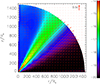 |
Fig. 1. Time-averaged logarithm of gas density (color scale) in g cm−3 and velocity (vectors) for ε = 0.8. The z-axis corresponds to the rotational axis of the accretion disk. The accretion disk surface is located in the z = 0 plane. |
We calculate the mass flux, kinetic power, and momentum flux of wind as a function of radius as follows:
 (11)
(11)
 (12)
(12)
 (13)
(13)
The results are shown in Figure 2. The wind is mainly launched and accelerated within 30Rs. Outside 30Rs, all fluxes remain constant with radius. The results demonstrate that the wind-launching and acceleration processes are complete within 30Rs. Nomura & Ohsuga (2017) performed simulations to study line-force-driven wind from an accretion disk in AGNs. They found that the wind in their simulations is launched mainly within 40Rs, which is very similar to the case in the present study. We test the impact of the TDE disk outer radius in Appendix C and find that changing the disk outer radius does not significantly affect the results. The wind is produced in two steps (Nomura & Ohsuga 2017). First, the gas is puffed up from the disk by the radiation pressure exerted by local UV photons. Second, the puffed-up gas is radially accelerated by line force to form the wind. We find that for a standard thin disk around a 106 M⊙ black hole, and considering an Eddington ratio around ε = 0.5, the UV photons from the region within 40Rs contribute to 80% of the total disk UV emission. Therefore, the disk gas inside 40Rs is more easily puffed up by radiation pressure. Outside 40Rs, UV disk emission is weak and the disk gas is very difficult to puff up to form a wind. Therefore, despite the disk size in AGNs being significantly larger than the disk in TDEs studied here, Nomura & Ohsuga (2017) find that the line-force-driven wind is also mainly launched very near the black hole.
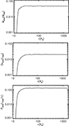 |
Fig. 2. Time-averaged radial profile of wind mass flux (top panel), kinetic power (middle panel), and momentum flux (bottom panel) for the model with ε = 0.8. |
The mass flux of the wind is 4.34% ṀEdd. Since the mass accretion rate is 80% ṀEdd, the ratio of the mass flux of the wind to the mass accretion rate is 5.4%. In the sub-Eddington accretion phase, more than 94% of the fallback stellar debris is accreted by the black hole. For comparison, in the super-Eddington accretion flow around a 106 M⊙ black hole in TDEs, 43% of the fallback debris is accreted (Bu et al. 2023b).
The kinematic power of the wind is ∼2.3 × 1042 erg/s. For comparison, in the super-Eddington phase, the kinematic power of the wind is well above 1044 erg/s (Bu et al. 2023b). The momentum flux of the wind is 12% that of the radiation from the thin disk, which is consistent with the fact that, for radiation-pressure-driven winds, the momentum flux is smaller than that of radiation.
We show the angular profile of the mass flux and radial velocity of the wind at the radial outer boundary in Figure 3. The main stream of the wind lies in the angular range 28° < θ < 45°, as shown in Figure 1. The maximum radial velocity reaches approximately 0.3c and occurs around ∼45°. The minimum wind velocity is ∼0.01c.
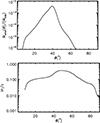 |
Fig. 3. Time-averaged angular profile of wind mass flux (top panel) and radial velocity (bottom panel) measured at the outer radial boundary for the model with ε = 0.8. |
3.2. Eddington ratio dependence
We also ran simulations with different values of ε. We find that when ε ≤ 0.2, the line force is too weak to launch a wind. Proga et al. (2000) and Proga & Kallman (2004) also found that when the Eddington ratio of the accretion disk is as low as 0.1, the winds did not appear.
In general, the angular distributions of the mass flux and the angular profiles of the wind velocity in models with different values of ε are quite similar to those shown in Figure 3. We show the mass flux and kinematic power of the wind in TDEs as a function of time (or mass accretion rate) in Figure 4. The top horizontal axis of this figure shows the time after the peak debris fallback rate. The time is calculated according to the equation  . For the parameters MBH = 106 M⊙ and M* = M⊙ used in this work, the transition from the super-Eddington fallback phase to the sub-Eddington fallback phase occurs at tcr = 760 days.
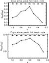 |
Fig. 4. Mass flux (top panel) and kinematic power (bottom panel) of wind measured at the outer radial boundary as a function of Eddington ratio. |
From 760 to 1549 days after the peak fallback rate, the mass flux lies in the range 1 − 6% ṀEdd. The kinematic power of the wind is in the range 1 − 6%LEdd. The wind reaches its maximum strength at ε = 0.6. As ε increases, the X-ray photon flux capable of photo-ionizing gas increases, leading to a higher ionization parameter. The line-force multiplier, ℳ, decreases as the ionization parameter increases. Therefore, when ε ≥ 0.6, strength of the wind decreases as ε increases. When ε < 0.6, the strength of the wind decreases as ε decreases, because a smaller ε results in a lower radiation flux and radiation pressure.
We time-integrate the mass and kinetic energy carried away by the wind from t = 760 to 1549 days. We find that during this period, the mass and kinetic energy carried away by the wind are 0.15% M⊙ and 1.6 × 1050 erg, respectively.
4. Discussion and observational applications
In the present study, we neglect the magnetic driven wind mechanism. The magnetic field likely significantly affects the evolution of the TDE disk. For example, Tamilan et al. (2025b) recently found that a strong magnetic field can cause the accretion rate to evolve as a t−5/2 law. Therefore, in the future, a t−5/2 law decline in radiation from TDEs may help to identify a TDE disk as magnetically dominated. To study magnetically driven winds, the geometry and strength of the magnetic field must be known. When magnetic field effects are included, the properties of the line-force-driven-winds may change. Yang (2021) report that when a weak poloidal large-scale magnetic field is present, both the wind velocity and the covering factor increase. This occurs because, in the presence of a magnetic field, the region around the rotational axis becomes magnetically pressure-dominated, which prevents gas from spreading to higher latitudes and enhances the gas column density at middle and low latitudes. A higher column density helps to shield X-ray photons, which causes the line force to be more effective in driving the wind. It remains unclear how the properties of line-force-driven winds behave in the presence of a small-scale tangled magnetic field. In reality, both magnetic fields and line forces contribute to driving winds. Therefore, future studies should investigate line-force-driven winds in the presence of a magnetic field in the context of TDEs.
The interaction of wind in TDEs with the CNM is believed to produce the radio emission observed in some TDEs (Alexander et al. 2020). We estimated the possible radio emission from the interaction of the line-force-driven wind with the CNM. This interaction can accelerate non-thermal electrons. Following the model of Matsumoto & Piran (2021), we calculated the radio emission luminosity using the wind primarily launched within the main stream at a polar angle range of ≈28° −45°, with an average velocity of 0.2c. We calculated the radio emission 1000 days after the wind launching. For the CNM, we adopted the model-dependent density profile of AT2019dsg given by Matsumoto & Piran (2024). The fractions of shocked thermal energy transferred to non-thermal electrons and magnetic fields were set to ϵe = ϵB = 0.1, with a non-thermal electron spectral index p = 2.5. In this scenario, the synchrotron self-absorption frequency is νa ∼ 3.4 GHz and the corresponding synchrotron luminosity is νLν ∼ 1040 erg s−1. The radio luminosity calculated here is sufficient to account for the observed radio emissions from TDEs (Alexander et al. 2020). Therefore, the line-force-driven wind can generate radio emission via wind-CNM interaction that is detectable with current telescopes. Future work should investigate this radio emission mechanism in greater detail.
Cold clouds may exist around SMBHs at galaxy centers. Observations of the Galactic center show a cold, dense circumnuclear disk on parsec scales (Zhao et al. 2016) and an inner “mini-spiral” (Tsuboi et al. 2016). Therefore, cold clouds and hot, diffuse CNM can coexist near quiescent SMBHs. Winds can collide with the cold, dense clouds that surround the SMBH. Bow shocks are induced, which accelerate power-law electrons (Mou et al. 2022; Bu et al. 2023a). In the wind-cloud model, the radio light curve can have a very steep rise (Mou et al. 2022). If the cloud distribution is highly non-uniform, strong fluctuations in the radio emission are expected These features differ from those predicted by the wind-CMN model. We estimated the radio emission for this scenario, adopting the same parameters as in the above outflow-CNM colliding model, including the fractions of shocked thermal energy transferred to non-thermal electrons and magnetic fields (ϵe = ϵB = 0.1). We assumed a wind velocity of 0.2c and calculated the radio emission 1000 days after the wind launch. The cloud was located at r ≈ vwindT = 5.2 × 1017 cm, with a cloud size (Rcloud = ηcloudr). The covering factor of the cloud was assumed to be cf = 0.2. The wind was primarily launched within a polar angle range of ≈28° −45°, with a kinetic power Lkin ≈ 2.3 × 1042 erg s−1. Under these conditions, we find that when ηcloud = 0.001, the synchrotron self-absorption frequency is νa = 0.1 GHz, and the corresponding radio luminosity is νLν = 4 × 1035 erg s−1. For ηcloud = 0.1, we obtain νa = 0.5 GHz, and the radio luminosity is νLν = 6 × 1037 erg s−1. For a cold cloud with a much larger size (ηcloud = 0.1), the radio emission produced by wind-cloud interactions can reach levels comparable to those observed with current telescopes (Alexander et al. 2020).
5. Summary
We investigated the line-force-driven wind from the sub-Eddington accretion disk around a 106 M⊙ black hole in TDEs. In our models, the accretion disk has a size of twice the pericenter radius, which is 47Rs, assuming a penetration factor β = 1 and the disruption of a solar type star.
We find that although the disk is small, strong wind is driven when the disk luminosity has an Eddington ratio ε > 0.2. The wind is mainly launched and accelerated within 30Rs. Beyond 30Rs, the mass flux, the kinetic power, and the momentum flux of the wind remain constant with radius. The maximum wind velocity reaches 0.3c. The disk wind has a mass flux in the range 1−6% ṀEdd The kinematic power of the wind lies in the range 1 − 6%LEdd. We briefly discuss the potential radio emission resulting from the interaction of the wind with the CNM or surrounding clouds.
Other models that explain the optical and UV emission of TDEs include the shock model (Piran et al. 2015; Jiang et al. 2016; Steinberg & Stone 2024; Huang et al. 2024; Guo et al. 2025) and the elliptical accretion model (Liu et al. 2017, 2021; Wevers et al. 2022).
We derive the scaling law for thin disk density in Equation (8) in Appendix B.
Acknowledgments
D. Bu is supported by the Natural Science Foundation of China (grants 12173065, 12133008, 12192220, 12192223). X. Yang is supported by Chongqing Natural Science Foundation (grant CSTB2023NSCQ-MSX0093) and the Natural Science Foundation of China (grant 12347101). L. Chen is supported by NSFC (12173066), National Key R&D program of China (2024YFA1611403), National SKA Program of China (2022SKA0120102) and Shanghai Pilot Programme for Basic Research, CAS Shanghai Branch (JCYJ-SHFY-2021-013). G. Mou is supported by the NSFC (grants 12473013, 12133007).
References
- Alexander, K. D., Berger, E., Guillochon, B. A., Zauderer, B. A., & Williams, P. K. G. 2016, ApJ, 819, L25 [NASA ADS] [CrossRef] [Google Scholar]
- Alexander, K. D., van Velzen, S., Horesh, A., & Zauderer, B. A. 2020, SSRv, 216, 81 [Google Scholar]
- Barniol Duran, R., Nakar, E., & Prian, T. 2013, ApJ, 772, 78 [NASA ADS] [CrossRef] [Google Scholar]
- Blandford, R. D., & Payne, D. G. 1982, MNRAS, 199, 883 [CrossRef] [Google Scholar]
- Bonnerot, C., Rossi, E. M., Lodaot, G., & Price, D. J. 2016, MNRAS, 455, 2253 [NASA ADS] [CrossRef] [Google Scholar]
- Bu, D., Qiao, E., Yang, X., et al. 2022, MNRAS, 516, 2833 [Google Scholar]
- Bu, D., Chen, L., Mou, G., Qiao, E., & Yang, X. 2023a, MNRAS, 521, 4180 [NASA ADS] [CrossRef] [Google Scholar]
- Bu, D., Qiao, E., & Yang, X. 2023b, MNRAS, 523, 4136 [Google Scholar]
- Cannizzo, J. K., Lee, H. M., & Goodman, J. 1990, ApJ, 351, 38 [NASA ADS] [CrossRef] [Google Scholar]
- Castor, J. I., Abbott, D. C., & Klein, R. I. 1975, ApJ, 195, 157 [Google Scholar]
- Cendes, Y., Alexander, K. D., Berger, E., et al. 2021, ApJ, 919, 127 [NASA ADS] [CrossRef] [Google Scholar]
- Cendes, Y., Berger, E., Alexander, K. D., et al. 2022, ApJ, 938, 28 [NASA ADS] [CrossRef] [Google Scholar]
- Cendes, Y., Berger, E., Alexander, K. D., et al. 2024, ApJ, 971, 185 [NASA ADS] [CrossRef] [Google Scholar]
- Cufari, M., Coughlin, E. R., & Nixon, C. J. 2022, ApJ, 924, 34 [NASA ADS] [CrossRef] [Google Scholar]
- Curd, B., & Narayan, R. 2019, MNRAS, 483, 565 [Google Scholar]
- Curd, B., & Narayan, R. 2023, MNRAS, 518, 3441 [Google Scholar]
- Dai, L., McKinney, J. C., Roth, N., Ramirez-Ruiz, E., & Miller, M. C. 2018, ApJ, 859, L20 [Google Scholar]
- Evans, C. R., & Kochanek, C. S. 1989, ApJ, 346, L13 [Google Scholar]
- Frank, J., King, A., & Raine, D. 1992, Camb. Astrophys. Ser., 21 [Google Scholar]
- Fukumura, K., Tombesi, F., Kazanas, D., et al. 2015, ApJ, 805, 17 [NASA ADS] [CrossRef] [Google Scholar]
- Gezari, S. 2021, ARA&A, 59, 21 [NASA ADS] [CrossRef] [Google Scholar]
- Golightly, E. C. A., Coughlin, E. R., & Nixon, C. J. 2019, ApJ, 872, 163 [NASA ADS] [CrossRef] [Google Scholar]
- Goodwin, A. J., van Velzen, S., Miller-Jones, J. C. A., et al. 2022, MNRAS, 511, 5328 [NASA ADS] [CrossRef] [Google Scholar]
- Guillochon, J., McCourt, M., Chen, X., Johnson, M. D., & Berger, E. K. G. 2016, ApJ, 822, 48 [NASA ADS] [CrossRef] [Google Scholar]
- Guo, H., Sun, J., Li, S., et al. 2025, ApJ, 979, 235 [Google Scholar]
- Hayasaki, K., & Yamazaki, R. 2023, ApJ, 954, 5 [Google Scholar]
- Hayasaki, K., Stone, N., & Loeb, A. 2013, MNRAS, 434, 909 [NASA ADS] [CrossRef] [Google Scholar]
- Hayasaki, K., Stone, N., & Loeb, A. 2016, MNRAS, 461, 3760 [NASA ADS] [CrossRef] [Google Scholar]
- Hayasaki, K., Zhong, S., Li, S., Berczik, P., & Spurzem, R. 2018, ApJ, 855, 129 [Google Scholar]
- Higginbottom, N., Scepi, N., Nicolas, K. C., et al. 2024, MNRAS, 527, 9236 [Google Scholar]
- Horesh, A., Cenko, S. B., & Arcavi, I. 2021, NatAs, 5, 491 [Google Scholar]
- Huang, X., Davis, S. W., & Jiang, Y. 2024, ApJ, 974, 165 [Google Scholar]
- Hung, T. e. a. 2017, ApJ, 842, 29 [NASA ADS] [CrossRef] [Google Scholar]
- Jiang, Y., Guillochon, J., & Loeb, A. 2016, ApJ, 830, 125 [NASA ADS] [CrossRef] [Google Scholar]
- Kato, S., Fukue, J., & Mineshige, S. 1978, Black-Hole Accretion Disks (Kyoto, Japan: Kyoto University Press) [Google Scholar]
- Komossa, S. 2015, JHEAp, 7, 148 [NASA ADS] [Google Scholar]
- Krolik, J., Piran, T., Svirski, G., & Cheng, R. M. 2016, ApJ, 827, 127 [NASA ADS] [CrossRef] [Google Scholar]
- Lei, X., Wu, Q., Li, H., et al. 2024, ApJ, 977, 63 [Google Scholar]
- Li, S. 2019, MNRAS, 490, 3793 [NASA ADS] [CrossRef] [Google Scholar]
- Li, S., & Begelman, M. C. 2014, ApJ, 786, 6 [NASA ADS] [CrossRef] [Google Scholar]
- Li, J., & Cao, X. 2022, ApJ, 926, 11 [Google Scholar]
- Liu, F., Zhou, Z., Cao, R., Ho, L. C., & Komossa, S. 2017, MNRAS, 472, L99 [NASA ADS] [CrossRef] [Google Scholar]
- Liu, F., Cao, C., Abramowicz, M. A., et al. 2021, ApJ, 908, 179 [Google Scholar]
- Lodato, G., & Rossi, E. M. 2011, MNRAS, 410, 359 [Google Scholar]
- Lodato, G., King, A. R., & Pringle, J. E. 2009, MNRAS, 392, 332 [NASA ADS] [CrossRef] [Google Scholar]
- Lu, W., & Bonnerot, C. 2020, MNRAS, 492, 686 [NASA ADS] [CrossRef] [Google Scholar]
- Lynden-Bell, D. 1996, MNRAS, 279, 389 [NASA ADS] [CrossRef] [Google Scholar]
- Mageshwaran, T., Shaw, G., & Bhattacharyya, S. 2023, MNRAS, 518, 5693 [Google Scholar]
- Matsumoto, T., & Piran, T. 2021, MNRAS, 507, 4196 [Google Scholar]
- Matsumoto, T., & Piran, T. 2023, MNRAS, 522, 4565 [Google Scholar]
- Matsumoto, T., & Piran, T. 2024, ApJ, 971, 49 [Google Scholar]
- Metzger, B. D., & Stone, N. C. 2016, MNRAS, 461, 948 [NASA ADS] [CrossRef] [Google Scholar]
- Mignone, A., Bodo, G., Massaglia, S., et al. 2007, ApJS, 170, 228 [Google Scholar]
- Mizumoto, M., Nomura, M., Done, C., Ohsuga, K., & Odaka, H. 2021, MNRAS, 503, 1442 [CrossRef] [Google Scholar]
- Mou, G., Wang, T., Wang, W., & Yang, J. 2022, MNRAS, 510, 3650 [Google Scholar]
- Murray, N., & Chiang, J. 1995, ApJ, 454, L105 [NASA ADS] [Google Scholar]
- Nomura, M., & Ohsuga, K. 2017, MNRAS, 465, 2873 [Google Scholar]
- Nomura, M., Ohsuga, K., Takahashi, H. R., Wada, K., & Yoshida, T. 2016, PASJ, 68, 16 [NASA ADS] [CrossRef] [Google Scholar]
- Ohsuga, K., Mori, M., Nakamoto, T., & Mineshige, S. 2005, ApJ, 628, 368 [NASA ADS] [CrossRef] [Google Scholar]
- Owocki, S. P., Castor, J. I., & Rybicki, G. B. 1988, ApJ, 335, 914 [NASA ADS] [CrossRef] [Google Scholar]
- Park, G., & Hayasaki, K. 2020, ApJ, 900, 3 [CrossRef] [Google Scholar]
- Parkinson, E. J., Kingge, C., Matthews, J. H., et al. 2022, MNRAS, 510, 5426 [Google Scholar]
- Perlman, E. S., Meyer, E. T., Wang, Q. D., et al. 2022, ApJ, 925, 143 [Google Scholar]
- Phinney, E. S. 1989, IAU Symp., 136, 543 [Google Scholar]
- Piran, T., Svirski, G., Krolik, J., Cheng, R. M., & Shiokawa, H. 2015, ApJ, 806, 164 [Google Scholar]
- Piro, A., & Lu, W. 2020, ApJ, 894, 2 [Google Scholar]
- Price, D. J., Liptai, D., Mandel, I., et al. 2024, ApJ, 971, L46 [NASA ADS] [CrossRef] [Google Scholar]
- Proga, D., & Kallman, T. R. 2004, ApJ, 616, 688 [Google Scholar]
- Proga, D., Stone, J. M., & Drew, J. E. 1998, MNRAS, 295, 595 [Google Scholar]
- Proga, D., Stone, J. M., & Kallman, T. R. 2000, ApJ, 543, 686 [Google Scholar]
- Rees, M. J. 1988, Nature, 333, 523 [Google Scholar]
- Reis, R. C., & Miller, J. M. 2013, ApJ, 769, 7 [NASA ADS] [CrossRef] [Google Scholar]
- Roth, N., Kasen, D., Guillochon, J., & Ramirez-Ruiz, E. 2016, ApJ, 827, 3 [Google Scholar]
- Rybicki, G. B., & Hummer, D. G. 1978, ApJ, 219, 654 [NASA ADS] [CrossRef] [Google Scholar]
- Sfaradi, I., Horesh, A., Fender, R., et al. 2022, ApJ, 933, 176 [Google Scholar]
- Sfaradi, I., Beniamini, P., Horesh, A., et al. 2024, MNRAS, 527, 7672 [Google Scholar]
- Shakura, N. I., & Sunyaev, R. A. 1973, A&A, 24, 337 [NASA ADS] [Google Scholar]
- Shiokawa, H., Krolik, J. H., Cheng, R. M., Piran, T., & Noble, S. C. 2015, ApJ, 804, 85 [Google Scholar]
- Steinberg, E., & Stone, N. C. 2024, Nature, 625, 463 [NASA ADS] [CrossRef] [Google Scholar]
- Strubbe, L. E., & Quataert, E. 2009, MNRAS, 400, 2070 [NASA ADS] [CrossRef] [Google Scholar]
- Tamilan, M., Hayasaki, K., & Suzuki, T. K. 2024, ApJ, 975, 94 [Google Scholar]
- Tamilan, M., Hayasaki, K., & Suzuki, T. K. 2025a, Prog. Theor. Exp. Phys., b3E02 [Google Scholar]
- Tamilan, M., Hayasaki, K., & Suzuki, T. K. 2025b, Prog. Theor. Exp. Phys., accepted [arXiv:2502.12549] [Google Scholar]
- Teboul, O., & Metzger, B. D. 2023, ApJ, 957, L9 [Google Scholar]
- Thomsen, L. L., Kwan, T., Dai, L., Wu, S., & Ramirez-Ruiz, E. 2022, ApJ, 937, L28 [NASA ADS] [CrossRef] [Google Scholar]
- Tsuboi, M., Kitamura, Y., Miyoshi, M., et al. 2016, PASJ, 68, 7 [Google Scholar]
- Uno, K., & Maeda, K. 2020, ApJ, 905, L5 [Google Scholar]
- Uttley, P., Cackett, E. M., Fabian, A. C., Kara, E., & Wilkins, D. R. 2014, A&ARv, 22, 72 [NASA ADS] [CrossRef] [Google Scholar]
- van Velzen, S., Holoien, T. W. S., Onori, F., Hung, T., & Arcavi, I. 2020, SSRv, 216, 124 [Google Scholar]
- Wang, W., Bu, D., & Yuan, F. 2022, MNRAS, 513, 5818 [NASA ADS] [CrossRef] [Google Scholar]
- Wevers, T., Nicholl, M., Guolo, M., et al. 2022, A&A, 666, 6 [Google Scholar]
- Yalinewich, A., Steinberg, E., Piran, T., & Krolik, J. H. 2019, MNRAS, 487, 4083 [Google Scholar]
- Yang, X. 2021, ApJ, 922, 262 [NASA ADS] [CrossRef] [Google Scholar]
- Yang, X., Ablimit, K., & Li, Q. 2021, ApJ, 914, 31 [Google Scholar]
- Yuan, F., Bu, D., & Wu, M. 2012, ApJ, 761, 130 [Google Scholar]
- Zhang, F., Shu, X., Yang, L., et al. 2024, ApJ, 962, L18 [NASA ADS] [CrossRef] [Google Scholar]
- Zhao, J., Morris, M. R., & Goss, W. M. 2016, ApJ, 817, L171 [Google Scholar]
- Zhong, S., Hayasaki, K., Li, S., Berczik, P., & Spurzem, R. 2023, ApJ, 959, 19 [Google Scholar]
- Zhou, C., Zhu, Z., Lei, W., et al. 2024, ApJ, 963, 66 [Google Scholar]
- Zhuang, J., Shen, R., Mou, G., & Lu, W. 2025, ApJ, 979, 109 [Google Scholar]
Appendix A: Line force multiplier
We adopt the CAK75 (Castor et al. 1975) analytical expression modified by Owocki et al. (1988) to calculate the force multiplier
![Mathematical equation: $$ \begin{aligned} \mathcal{M} (t) = kt^{-\alpha }\left[\frac{(1+\tau _{\rm max})^{1-\alpha }-1}{\tau _{\rm max}^{1-\alpha }}\right] \end{aligned} $$](/articles/aa/full_html/2026/01/aa56161-25/aa56161-25-eq18.gif) (A.1)
(A.1)
t is a function of the optical depth parameter defined as
 (A.2)
(A.2)
where σe is the mass-scattering coefficient for free electrons, vth is the thermal velocity and dvl/dl is the velocity gradient along the line of sight  . In equation (A.1), k is proportional to the total number of lines and calculated as
 (A.3)
(A.3)
where ξ is the ionization parameter defined in Section 2.1. α = 0.6 is the ratio of optically thick to optically thin lines and does not change with ξ. τmax = tηmax and
 (A.4)
(A.4)
 (A.5)
(A.5)
The line force also becomes negligible if gas temperature T > 105 K for any value of ξ (Proga et al. 2000).
Appendix B: Derivation of the scaling law for the thin disk density in Equation 8
The basic equations of the thin disk are as follows (Frank et al. 1992),
 (B.1)
(B.1)
 (B.2)
(B.2)
 (B.3)
(B.3)
 (B.4)
(B.4)
 (B.5)
(B.5)
 (B.6)
(B.6)
 (B.7)
(B.7)
 (B.8)
(B.8)
In above equations,  is the density of the disk, Σ is the surface density, H is the scale height, Cs is the sound speed, p is the pressure including the gas pressure and radiation pressure, k is the Boltzmann constant, Tc is the disk temperature, σ is the Stefan-Boltzmann constant, τ is the optical depth, κ is the opacity, ν is the kinematic viscosity and α is the viscosity coefficient.
Substituting Equations (B.1) and (B.8) into Equation (B.7), we have,
 (B.9)
(B.9)
In the inner region, only considering radiation pressure (p ∝ Tc4) and using Equation (B.5), we have,
 (B.10)
By using Equation (B.3), we have,
 (B.11)
Combining Equations (B.2) and (B.11), we have,
 (B.12)
Combing Equations (B.2), (B.9) and (B.12), we have,
 (B.13)
Expressing Ṁ with the Eddington accretion rate  , we have,
 (B.14)
Because Rs ∝ MBH, Equation (B.14) becomes,
 (B.15)
which is the scaling law used in Equation (8).
Appendix C: Dependence on physical parameters
C.1. The inner radial boundary
We test the effects of radial inner boundary. In this test, we fix the Eddington ratio of disk luminosity to be ε = 0.8. In our fiducial model, we have an inner radial boundary of 10Rs. We run two test simulations with inner radial boundary at 15Rs and 20Rs, respectively. We show the radial profiles of the wind mass flux in Figure C.1. At the outer radial boundary, the mass flux of wind differs by a factor smaller than 10%. Slightly changing the inner radial boundary would not affect the results much.
C.2. The disk outer boundary
We test the effects of TDE disk outer boundary. In this test, we fix the Eddington ratio of disk luminosity to be ε = 0.8. In our fiducial model, we have a disk outer boundary of 47Rs. We run a test simulation with the TDE disk outer boundary at 100Rs. We show the radial profiles of the wind mass flux in Figure C.2. We can see that the radial profiles of the two models are roughly same. Therefore, changing the outer boundary of the TDE disk in reasonable regime would not affect the results.
C.3. The ratio of X-ray luminosity to disk luminosity
We test the effects of the value of fX. In this test, we fix the Eddington ratio of disk luminosity to be ε = 0.8. In our fiducial model, we have fX = 0.03. Li (2019) studied a sample of luminous AGNs. Generally, they found that the ratio of the X-ray luminosity to the bolometric luminosity decreases with the Eddington ratio ε. In their table 2, for the AGNs with Eddington ratios in the range 0.3-1.0, the value of fX is in the range of 0.015-0.05. Therefore, we run two test simulations with fX = 0.015 and fX = 0.05, respectively. We show the radial profiles of the wind mass flux in Figure C.3. Generally, the line force multiplier decreases with the increase of fX. With fixed UV radiation flux, the line force decreases with the increase of fX. Therefore, we can see that the mass flux of wind decreases with the increase of fX. However, there is just little change of wind flux. Compared to the fiducial model with fX = 0.03, the wind mass flux is changed by a factor smaller than 1.
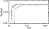 |
Fig. C.1. Time-averaged radial profiles of wind mass flux for models with inner radial boundary at 10Rs (solid line, fiducial model in Section 3.1), 15Rs (dotted line) and 20Rs (dashed line) with ε = 0.8. |
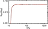 |
Fig. C.2. Time-averaged radial profile of wind mass flux for models with TDE disk outer boundary at 47Rs (black solid line, fiducial model in Section 3.1), 100Rs (red dashed line) with ε = 0.8. |
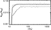 |
Fig. C.3. Time-averaged radial profile of wind mass flux for models with fX = 0.03 (solid line, fiducial model in Section 3.1), fX = 0.015 (dotted line) and fX = 0.05 (dashed line) with ε = 0.8. |
Appendix D: The Eddington ratio dependence of line force
In section 3.2, we find that the wind is strongest when ε = 0.6. The reason is as follows discussed in Secton 3.2. With the increase of ε, the X-ray flux increases, which will result in high ionization parameter. We show the results of the radial profiles of gas ionization parameter at a snapshot when the simulations achieves quasi-steady states for an angular position at θ = 82° close to the wind launching mid-plane in Figure D.1. It is clear that higher ε results in higher ionization parameter.
We show the corresponding radial profiles of line force multiplier in Figure D.2. The force multiplier is not continuous with radius. At some positions the multiplier is zero. The reason is that as motioned above (in Appendix A), the multiplier is zero when the gas temperature is higher than 105 K (Proga et al. 2000). The region with zero multiplier has gas temperature higher than 105K. We focus on the winds launching and accelerating region (r < 30Rs). It can be seen that generally the force multiplier increases with decreasing ε (or ionization parameter).
The corresponding radial component of the line forces are shown in Figure D.3. The radial component of line force accelerates wind radially. It can be seen that within the wind launching region r < 30Rs, the line force is strongest in model with ε = 0.6, which has strongest wind. Therefore, as explained in Section 3.2, the reason for the strongest wind in model with ε = 0.6 is as follows. With the increase of ε, the ionization parameter of gas increases. The line force multiplier decreases with increasing ionization parameter. Therefore, when ε ≥ 0.6, the strength of wind decreases with increase of ε. When ε < 0.6, the strength of wind decreases with decreasing of ε. The reason is that smaller ε results in a smaller radiation flux and radiation pressure.
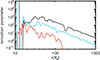 |
Fig. D.1. Radial profiles of gas ionization parameter at a snapshot when the simulations achieves quasi-steady states. The figure is for an angular position at θ = 82° close to the wind launching mid-plane. The black, blue and red lines correspond to models (introduced in Section 3) of ε = 0.8, ε = 0.6 and ε = 0.4, respectively. |
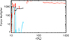 |
Fig. D.2. Radial profiles of line force multiplier at a snapshot when the simulations achieves quasi-steady states. The figure is for an angular position at θ = 82° close to the wind launching mid-plane. The black, blue and red lines correspond to models (introduced in Section 3) of ε = 0.8, ε = 0.6 and ε = 0.4, respectively. |
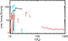 |
Fig. D.3. Radial profiles of radial component of the line force at a snapshot when the simulations achieves quasi-steady states. The figure is for an angular position at θ = 82° close to the wind launching mid-plane. The black, blue and red lines correspond to models (introduced in Section 3) of ε = 0.8, ε = 0.6 and ε = 0.4, respectively. |
We plot the radial profile of the radial component of the line force of the model with ε = 0.2 (discussed in Section 3) in Figure D.4. The plot is for an angular position of θ = 85° close to the wind launching mid-plane. It is clear that in this model, the radial line force is much smaller than black hole gravity. Winds can not be driven in this model.
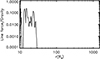 |
Fig. D.4. Radial profile of radial component of the line force at a snapshot when the simulation achieves quasi-steady states for the model with ε = 0.2 (see Section 3). The figure is for an angular position at θ = 85° close to the wind launching mid-plane. |
All Figures
|
Fig. 1. Time-averaged logarithm of gas density (color scale) in g cm−3 and velocity (vectors) for ε = 0.8. The z-axis corresponds to the rotational axis of the accretion disk. The accretion disk surface is located in the z = 0 plane. |
| In the text | |
|
Fig. 2. Time-averaged radial profile of wind mass flux (top panel), kinetic power (middle panel), and momentum flux (bottom panel) for the model with ε = 0.8. |
| In the text | |
|
Fig. 3. Time-averaged angular profile of wind mass flux (top panel) and radial velocity (bottom panel) measured at the outer radial boundary for the model with ε = 0.8. |
| In the text | |
|
Fig. 4. Mass flux (top panel) and kinematic power (bottom panel) of wind measured at the outer radial boundary as a function of Eddington ratio. |
| In the text | |
|
Fig. C.1. Time-averaged radial profiles of wind mass flux for models with inner radial boundary at 10Rs (solid line, fiducial model in Section 3.1), 15Rs (dotted line) and 20Rs (dashed line) with ε = 0.8. |
| In the text | |
|
Fig. C.2. Time-averaged radial profile of wind mass flux for models with TDE disk outer boundary at 47Rs (black solid line, fiducial model in Section 3.1), 100Rs (red dashed line) with ε = 0.8. |
| In the text | |
|
Fig. C.3. Time-averaged radial profile of wind mass flux for models with fX = 0.03 (solid line, fiducial model in Section 3.1), fX = 0.015 (dotted line) and fX = 0.05 (dashed line) with ε = 0.8. |
| In the text | |
|
Fig. D.1. Radial profiles of gas ionization parameter at a snapshot when the simulations achieves quasi-steady states. The figure is for an angular position at θ = 82° close to the wind launching mid-plane. The black, blue and red lines correspond to models (introduced in Section 3) of ε = 0.8, ε = 0.6 and ε = 0.4, respectively. |
| In the text | |
|
Fig. D.2. Radial profiles of line force multiplier at a snapshot when the simulations achieves quasi-steady states. The figure is for an angular position at θ = 82° close to the wind launching mid-plane. The black, blue and red lines correspond to models (introduced in Section 3) of ε = 0.8, ε = 0.6 and ε = 0.4, respectively. |
| In the text | |
|
Fig. D.3. Radial profiles of radial component of the line force at a snapshot when the simulations achieves quasi-steady states. The figure is for an angular position at θ = 82° close to the wind launching mid-plane. The black, blue and red lines correspond to models (introduced in Section 3) of ε = 0.8, ε = 0.6 and ε = 0.4, respectively. |
| In the text | |
|
Fig. D.4. Radial profile of radial component of the line force at a snapshot when the simulation achieves quasi-steady states for the model with ε = 0.2 (see Section 3). The figure is for an angular position at θ = 85° close to the wind launching mid-plane. |
| In the text | |
Current usage metrics show cumulative count of Article Views (full-text article views including HTML views, PDF and ePub downloads, according to the available data) and Abstracts Views on Vision4Press platform.
Data correspond to usage on the plateform after 2015. The current usage metrics is available 48-96 hours after online publication and is updated daily on week days.
Initial download of the metrics may take a while.