| Issue |
A&A
Volume 705, January 2026
|
|
|---|---|---|
| Article Number | A138 | |
| Number of page(s) | 12 | |
| Section | Astronomical instrumentation | |
| DOI | https://doi.org/10.1051/0004-6361/202556173 | |
| Published online | 16 January 2026 | |
Euclid: methodology for derivation of IPC-corrected conversion gain of nonlinear CMOS APS★
1
Aix-Marseille Université, CNRS/IN2P3, CPPM,
Marseille,
France
2
Université Claude Bernard Lyon 1,
CNRS/IN2P3, IP2I Lyon, UMR 5822,
Villeurbanne
69100,
France
3
INAF-Osservatorio Astronomico di Brera,
Via Brera 28,
20122
Milano,
Italy
4
Dipartimento di Fisica e Astronomia, Università di Bologna,
Via Gobetti 93/2,
40129
Bologna,
Italy
5
INAF-Osservatorio di Astrofisica e Scienza dello Spazio di Bologna,
Via Piero Gobetti 93/3,
40129
Bologna,
Italy
6
INFN-Sezione di Bologna,
Viale Berti Pichat 6/2,
40127
Bologna,
Italy
7
INAF-Osservatorio Astrofisico di Torino,
Via Osservatorio 20,
10025
Pino Torinese (TO),
Italy
8
Dipartimento di Fisica, Università di Genova,
Via Dodecaneso 33,
16146
Genova,
Italy
9
INFN-Sezione di Genova,
Via Dodecaneso 33,
16146
Genova,
Italy
10
Department of Physics “E. Pancini”, University Federico II,
Via Cinthia 6,
80126
Napoli,
Italy
11
INAF-Osservatorio Astronomico di Capodimonte,
Via Moiariello 16,
80131
Napoli,
Italy
12
INFN section of Naples,
Via Cinthia 6,
80126
Napoli,
Italy
13
Instituto de Astrofísica e Ciências do Espaço, Universidade do Porto,
CAUP, Rua das Estrelas,
PT4150-762
Porto,
Portugal
14
Faculdade de Ciências da Universidade do Porto,
Rua do Campo de Alegre,
4150-007
Porto,
Portugal
15
Aix-Marseille Université, CNRS, CNES, LAM,
Marseille,
France
16
Dipartimento di Fisica, Università degli Studi di Torino,
Via P. Giuria 1,
10125
Torino,
Italy
17
INFN-Sezione di Torino,
Via P. Giuria 1,
10125
Torino,
Italy
18
INAF-IASF Milano,
Via Alfonso Corti 12,
20133
Milano,
Italy
19
Centro de Investigaciones Energéticas, Medioambientales y Tecnológicas (CIEMAT),
Avenida Complutense 40,
28040
Madrid,
Spain
20
Port d’Informació Científica,
Campus UAB, C. Albareda s/n,
08193
Bellaterra (Barcelona),
Spain
21
Institute for Theoretical Particle Physics and Cosmology (TTK), RWTH Aachen University,
52056
Aachen,
Germany
22
INAF-Osservatorio Astronomico di Roma,
Via Frascati 33,
00078
Monteporzio Catone,
Italy
23
Dipartimento di Fisica e Astronomia “Augusto Righi” - Alma Mater Studiorum Università di Bologna,
Viale Berti Pichat 6/2,
40127
Bologna,
Italy
24
Instituto de Astrofísica de Canarias, Vía Láctea,
38205
La Laguna,
Tenerife,
Spain
25
Institute for Astronomy, University of Edinburgh, Royal Observatory,
Blackford Hill,
Edinburgh
EH9 3HJ,
UK
26
Jodrell Bank Centre for Astrophysics, Department of Physics and Astronomy, University of Manchester,
Oxford Road,
Manchester
M13 9PL,
UK
27
European Space Agency/ESRIN,
Largo Galileo Galilei 1,
00044
Frascati,
Roma,
Italy
28
ESAC/ESA,
Camino Bajo del Castillo, s/n., Urb. Villafranca del Castillo,
28692
Villanueva de la Cañada,
Madrid,
Spain
29
Institute of Physics, Laboratory of Astrophysics, Ecole Polytechnique Fédérale de Lausanne (EPFL), Observatoire de Sauverny,
1290
Versoix,
Switzerland
30
Institut de Ciències del Cosmos (ICCUB), Universitat de Barcelona (IEEC-UB),
Martí i Franquès 1,
08028
Barcelona,
Spain
31
Institució Catalana de Recerca i Estudis Avançats (ICREA),
Passeig de Lluís Companys 23,
08010
Barcelona,
Spain
32
UCB Lyon 1, CNRS/IN2P3, IUF, IP2I Lyon,
4 rue Enrico Fermi,
69622
Villeurbanne,
France
33
Departamento de Física, Faculdade de Ciências, Universidade de Lisboa,
Edifício C8, Campo Grande,
PT1749-016
Lisboa,
Portugal
34
Instituto de Astrofísica e Ciências do Espaço, Faculdade de Ciên-cias, Universidade de Lisboa,
Campo Grande,
1749-016
Lisboa,
Portugal
35
Université Paris-Saclay, CNRS, Institut d’astrophysique spatiale,
91405
Orsay,
France
36
Department of Astronomy, University of Geneva,
ch. d’Ecogia 16,
1290
Versoix,
Switzerland
37
INFN-Padova,
ViaMarzolo 8,
35131
Padova,
Italy
38
INAF-Istituto di Astrofisica e Planetologia Spaziali,
via del Fosso del Cavaliere, 100,
00100
Roma,
Italy
39
Université Paris-Saclay, Université Paris Cité, CEA, CNRS, AIM,
91191
Gif-sur-Yvette,
France
40
Space Science Data Center, Italian Space Agency,
via del Politecnico snc,
00133
Roma,
Italy
41
INAF-Osservatorio Astronomico di Trieste,
Via G. B. Tiepolo 11,
34143
Trieste,
Italy
42
Istituto Nazionale di Fisica Nucleare, Sezione di Bologna,
Via Irnerio 46,
40126
Bologna,
Italy
43
Max Planck Institute for Extraterrestrial Physics,
Giessenbachstr. 1,
85748
Garching,
Germany
44
Universitäts-Sternwarte München, Fakultät für Physik, Ludwig-Maximilians-Universität München,
Scheinerstrasse 1,
81679
München,
Germany
45
Institute of Theoretical Astrophysics, University of Oslo,
PO Box 1029
Blindern,
0315
Oslo,
Norway
46
Jet Propulsion Laboratory, California Institute of Technology,
4800 Oak Grove Drive,
Pasadena,
CA,
91109,
USA
47
Felix Hormuth Engineering,
Goethestr. 17,
69181
Leimen,
Germany
48
Technical University of Denmark,
Elektrovej 327, 2800 Kgs.
Lyngby,
Denmark
49
Cosmic Dawn Center (DAWN),
Denmark
50
Institut d’Astrophysique de Paris, UMR 7095, CNRS, and Sorbonne Université,
98 bis boulevard Arago,
75014
Paris,
France
51
Max-Planck-Institut für Astronomie,
Königstuhl 17,
69117
Heidelberg,
Germany
52
NASA Goddard Space Flight Center,
Greenbelt,
MD
20771,
USA
53
Department of Physics,
PO Box 64,
00014
University of Helsinki,
Finland
54
Helsinki Institute of Physics,
Gustaf Hällströmin katu 2, University of Helsinki,
Helsinki,
Finland
55
NOVA optical infrared instrumentation group at ASTRON,
Oude Hoogeveensedijk 4,
7991PD,
Dwingeloo,
The Netherlands
56
Centre de Calcul de l’IN2P3/CNRS,
21 avenue Pierre de Coubertin
69627
Villeurbanne Cedex,
France
57
Dipartimento di Fisica “Aldo Pontremoli”, Università degli Studi di Milano,
Via Celoria 16,
20133
Milano,
Italy
58
INFN-Sezione di Milano,
Via Celoria 16,
20133
Milano,
Italy
59
Universität Bonn, Argelander-Institut für Astronomie,
Auf dem Hügel 71,
53121
Bonn,
Germany
60
Dipartimento di Fisica e Astronomia “Augusto Righi” - Alma Mater Studiorum Università di Bologna,
via Piero Gobetti 93/2,
40129
Bologna,
Italy
61
Department of Physics, Centre for Extragalactic Astronomy, Durham University,
South Road,
Durham,
DH1 3LE,
UK
62
Université Paris Cité, CNRS, Astroparticule et Cosmologie,
75013
Paris,
France
63
European Space Agency/ESTEC,
Keplerlaan 1,
2201 AZ
Noordwijk,
The Netherlands
64
School of Mathematics, Statistics and Physics, Newcastle University,
Herschel Building,
Newcastle-upon-Tyne,
NE1 7RU,
UK
65
Institut de Física d’Altes Energies (IFAE), The Barcelona Institute of Science and Technology,
Campus UAB,
08193
Bellaterra (Barcelona),
Spain
66
DARK, Niels Bohr Institute, University of Copenhagen,
Jagtvej 155,
2200
Copenhagen,
Denmark
67
Centre National d’Etudes Spatiales - Centre spatial de Toulouse,
18 avenue Edouard Belin,
31401
Toulouse Cedex 9,
France
68
Institute of Space Science,
Str. Atomistilor, nr. 409 Magurele,
Ilfov
077125,
Romania
69
Dipartimento di Fisica e Astronomia “G. Galilei”, Università di Padova,
Via Marzolo 8,
35131
Padova,
Italy
70
Departamento de Física, FCFM, Universidad de Chile,
Blanco Encalada
2008,
Santiago,
Chile
71
Infrared Processing and Analysis Center, California Institute of Technology,
Pasadena,
CA
91125,
USA
72
Instituto de Astrofísica e Ciências do Espaço, Faculdade de Ciên-cias, Universidade de Lisboa,
Tapada da Ajuda,
1349-018
Lisboa,
Portugal
73
Universidad Politécnica de Cartagena, Departamento de Electrónica y Tecnología de Computadoras,
Plaza del Hospital 1,
30202
Cartagena,
Spain
74
Institut de Recherche en Astrophysique et Planétologie (IRAP), Université de Toulouse, CNRS, UPS, CNES,
14 Av. Edouard Belin,
31400
Toulouse,
France
75
INFN-Bologna,
Via Irnerio 46,
40126
Bologna,
Italy
76
Dipartimento di Fisica, Università degli studi di Genova, and INFN-Sezione di Genova,
via Dodecaneso 33,
16146
Genova,
Italy
★★ Corresponding author: This email address is being protected from spambots. You need JavaScript enabled to view it.
Received:
30
June
2025
Accepted:
5
October
2025
Abstract
We introduce a fast method to measure the conversion gain in complementary metal-oxide-semiconductor active pixel sensors, which accounts for nonlinearity and interpixel capacitance (IPC). The standard “mean-variance” method is biased because it assumes that pixel values depend linearly on the signal, and existing methods to correct for nonlinearity still introduce significant biases. While current IPC correction methods are prohibitively slow for a per-pixel application, our new method uses separate measurements of the IPC kernel to calculate the gain almost instantaneously. Using test data from a flight detector of the ESA Euclid mission, the IPC correction recovers the results of slower methods with 0.1% accuracy. The nonlinearity correction ensures that the estimated gain is independent of signal, correcting a bias of more than 2.5%.
Key words: instrumentation: detectors / methods: data analysis / methods: numerical / methods: statistical
This paper is published on behalf of the Euclid Consortium.
© The Authors 2026
 Open Access article, published by EDP Sciences, under the terms of the Creative Commons Attribution License (https://creativecommons.org/licenses/by/4.0), which permits unrestricted use, distribution, and reproduction in any medium, provided the original work is properly cited.
This article is published in open access under the Subscribe to Open model. This email address is being protected from spambots. You need JavaScript enabled to view it. to support open access publication.
1 Introduction
Since the early 2000s, considerable efforts have been made to enhance the sensitivity of complementary metal-oxide-semiconductor (CMOS) imaging sensors (Fossum 1997). Currently, the industry produces large-format CMOS active pixel sensors (APS) exceeding one thousand pixels on each side,which exhibit ultra-low noise and sensitivity ranging from UV to long-wavelength infrared (LWIR). Thanks to these advancements, CMOS APS are highly suitable for low-light imaging across various wavelengths, making them ideal for both astronomical and cosmological observations.
Although CMOS APS with silicon-sensitive layers have been used in UV (Greffe et al. 2022) and visible light applications (Soman et al. 2015), their most extensive development has been in the IR wavelength range. Many CMOS APS designed for IR applications employ HgCdTe as the sensitive layer, exploiting its tunable bandgap (Rogalski 2011), which is adjusted by varying the alloy composition. Several companies have developed high-performance sensors, such as Raytheon with the VIRGO sensor (Bezawada et al. 2004) and LYNRED with the ALFA sensor for “Astronomy Large Format Array” (Gravrand et al. 2022). Nevertheless, the most widely used sensors in astronomical or cosmological missions are the HxRG series by Teledyne. These detectors play a crucial role in numerous observatories. For example, the H1RG model will be used in the ARIEL mission dedicated to exoplanet studies (Pichon et al. 2022) and in the MAJIS instrument of the JUICE mission (Cisneros-González et al. 2020). Teledyne detectors are deployed both in space for low light imaging missions - including the large H2RG-based focal plane array of the Euclid NISP spectro-photometer (Euclid Collaboration 2025b,a; Secroun et al. 2016), the four H2RG-based instruments of JWST (Rauscher et al. 2014), and the H4RG-based spectro-imager of the Nancy Grace Roman Space Telescope (Mosby et al. 2020) -, and in ground-based observatories, including many instruments of the Extremely Large Telescope (ELT)(Bezawada et al. 2023). Recently, CMOS APS based on avalanche photodiodes (APD), developed by the Leonardo company in collaboration with ESA and NASA (Claveau et al. 2022), have achieved performance comparable to classical HgCdTe sensors with large-format arrays.
Regardless of the wavelength range, design, or scientific application, sensor performance is generally evaluated through three fundamental parameters: quantum efficiency (QE), readout noise, and dark current. These parameters are also used in pipelines to compute science data products. Assessing their absolute values requires expressing them in physical units (electrons) rather than arbitrary digital units (ADUs) - the standard unit of raw data. The conversion gain, defined as the number of electrons represented by one ADU, is a crucial sensor parameter, and inaccuracies in gain estimation may bias other sensor parameters. A striking example quantum efficiency (QE), evaluated as the ratio of charges collected by the photodiode to incident photons. Standard methods for measuring QE involve observing changes in ADU under calibrated photon flux. Consequently, to obtain an absolute QE value, the conversion gain must be accurately determined, as any bias in gain measurement propagates to the estimated QE.
Since conversion gain directly impacts sensor performance, its measurement is subject to several technical requirements. In particular, with recent missions such as Euclid and ARIEL (Atmospheric Remote-Sensing Infrared Exoplanet Large-survey) pursuing ambitious scientific objectives, the required accuracy for conversion gain has increased significantly. For example, the QE of the ARIEL Infrared Spectrometer detector must be measured to an accuracy better than 0.5%, a requirement that directly constrains the uncertainty on the conversion gain. Similarly, the Euclid mission requires photon signal estimates to be accurate within 1%, which increases the demands on gain precision. Finally, these missions specify a minimum fraction of operable pixels - 95% for Euclid - with operability defined by performance thresholds such as QE, dark current, and readout noise. As a result, conversion gain must be measured at the pixel level. These combined requirements impose stringent constraints on the characterization of the conversion gain.
One of the most challenging aspects of gain measurement is that gain functions as a black box. Within this black box, several physical processes may take place, making the measurement sensitive to correlations with several other parameters, as well as environmental conditions. For instance, any correlation in the signal of closed pixels biases the measurement of conversion gain (Moore et al. 2006). A known source of such spatial correlation is electric cross-talk between neighboring pixels due to their proximity, referred to as interpixel capacitance (IPC). Moreover, since the gain must be measured per pixel, this IPC-induced bias on gain also needs to be measured per pixel, rendering existing methods (detailed in Sect. 2.3) hardly applicable. Similarly, the temporal correlation arising from signal persistence (detailed in Sect. 2.3) complicates gain measurements. Finally, although no published evidence suggests dependence on sensor temperature or photon wavelength, the signal dependence of gain measurement is well documented (detailed in Sect. 4.1) and remains problematic. Consequently, using acquisitions with different signal levels yields different measurements of conversion gain, introducing systematic uncertainties that can easily exceed the required accuracy. Given these challenges, there is a clear need for a reliable method to measure an unbiased conversion gain at the pixel level, one that is decoupled from all other parameters.
The aim of this work is to propose a new, easily applicable method to measure a conversion gain that is decorrelated from IPC and independent of the signal level used during acquisition. In Sect. 2, we detail the concept of conversion gain, explore classical measurement methods, and discuss their limitations, which motivate the need for a new method of gain derivation. In Sect. 3, we propose and validate a new per-pixel correction of IPC bias in gain measurement. Finally, in Sect. 4, we introduce a new “nonlinear” mean-variance method, an original derivation of the relation between signal variance and mean, which allows us to estimate a signal-independent conversion gain. As this work forms part of the Euclid IR detector characterization conducted at the Center for Particle Physics of Marseille (CPPM), the validation of both methods is based on on-ground characterization data from CPPM campaigns (a detailed description of these data can be found in Secroun et al. 2016).
2 Conversion gain
2.1 Conversion gain measurement
Despite some design variations, CMOS APS broadly share a similar architectural framework, and their simplified design can be described as follows. Each pixel primarily comprises a photodiode (typically a reverse-biased p-n junction) for charge photo-generation. This photodiode, potentially followed by a multiplication region as in the case of APDs, interfaces with the readout integrated circuit (ROIC) via an indium bump. The ROIC structure may vary (e.g., source follower or capacitive transimpedance amplifier Guellec et al. 2017) and uses transistors to amplify and buffer the voltage signal. At the ROIC output, another buffer interfaces with external readout electronics, which generally include at least one analog-to-digital converter (ADC) channel to digitize the output voltage signal into ADUs. Owing to this architecture, the charge in each pixel can be read non-destructively. To reduce readout noise, each pixel is sampled repeatedly, generating a “ramp” of signal that can be processed using various techniques to estimate the flux (Rauscher et al. 2007). The conversion gain, expressed in electrons per ADU (e− ADU−1), is the ratio of the number of electrons accumulated by the photodiode to the number of ADUs generated by the ADC. This gain is typically considered as the combination of three distinct processes: the charge-to-voltage conversion from electrons to volts in the photodiode, the amplification and buffering from volts to volts in the ROIC, and the ADC conversion from volts to ADUs in the external electronics. Given its criticality in CMOS APS performance, considerable effort has been dedicated to accurately measuring conversion gain, leading to the development of various techniques. The capacitance comparison method (Finger et al. 2005) enables precise measurement of conversion gain but requires the addition of a finely calibrated external capacitance. The Fe55 technique, commonly used for Charge-Coupled Devices (CCDs) (Fraser et al. 1994), has been adapted for CMOS APS (Fox et al. 2009). However, measuring the conversion gain across all pixels with these techniques is tedious and therefore seldom used. Ultimately, the most prevalent method for measuring conversion gain involves flat-field acquisition, where all pixels are uniformly illuminated. Subsequently, the application of existing analytical methods based on statistical descriptions of the pixel response enables the conversion gain of each pixel to be measured.
Recent studies (Hendrickson & Haefner 2023) have introduced methods that use sophisticated statistical descriptions of signal output to approximate measured distributions. These methods are specifically optimized for sub-electron readout noise detectors, such as APDs, making them less applicable to more common detectors with read noise ranging from a few electrons to tens of electrons. For these common detectors, the “gold standard” flat-field gain measurement method was initially proposed by Mortara & Fowler (1981) as the “mean variance” method and later refined by Janesick (2001) into the well-known “photon transfer curve” (PTC). These methods are based on the derivation of the mean-variance equation relating the variance and mean of a pixel’s output signal. They assume that for a linear sensor, the output signal S (ADU) of a pixel that has integrated a charge Q (e−) is given by
 (1)
(1)
where g denotes the conversion gain in e− ADU−1. Here, the readout noise does not appear, as it is assumed to be Gaussian noise with a mean of zero and a standard deviation of σr.
Assuming that g is constant and that Q does not depend on g, the variance  of the signal can be calculated by applying the error-propagation formula to Eq. (1). The readout noise σr is added in quadrature in the variance equation
 (2)
(2)
Finally, assuming Poisson-distributed integrated electrons (σQ = Q) and negligible conversion gain variance σg, the total variance is expressed as
 (3)
(3)
According to Eq. (3), the conversion gain may be accurately determined by linear fitting of the mean-variance curve constructed from flat-field measurements. Typically, a meanvariance curve is constructed from a series of M similar flat-field ramps. Within these ramps, the signal variance and mean are estimated across the M ramps for each pixel. As the ramps consist of measurements spaced by uniform integration times, the mean-variance curve contains the same number of data points as there are measurements in a ramp. The gain is then derived as the inverse slope of the expected linear relationship, with the readout noise determined as its intercept.
2.2 Uncertainty on gain measurement
Although some authors (Beecken & Fossum 1996) have attempted to estimate the uncertainty associated with conversion gain measurements using the mean-variance method, the practical difficulty in assessing the uncertainty of the variance used to construct the curve, followed by the fitting process, renders precise estimation challenging. Therefore, the conventional approach to uncertainty estimation involves repeating the measurement of the gain of a single pixel and using the resulting mean as a gain estimator, with the standard error of the sample mean,  , as the uncertainty estimator. Here, N represents the number of gain measurements and σg denotes their standard deviation. The challenge arises because M ramps are needed to perform a single gain measurement, and subsequently, N gain measurements require N × M ramps to estimate both the gain and the error. This requirement considerably increases the total number of acquisitions. For instance, aiming for an uncertainty of 1%, as required for the Euclid mission, and choosing to measure variance and mean across 50 ramps of 400 frames necessitates approximately 500 gain measurements, corresponding to 25 000 ramps, taking approximately 4000 hours (almost six months) for Euclid detectors-an impractical number. This estimation comes from a Monte Carlo simulation of an ideal linear sensor. One way to limit the number of ramps required is to combine spatial and temporal statistics by applying the ergodic hypothesis at small scales. This involves assuming that the gain is the same for a box of P×P pixels, called a superpixel, and that the signal values in the P×P pixels are uncorrelated. Then, instead of 50, only a pair of ramps acquired under the same conditions (such as flux, integration time, and temperature) are required to measure a per-superpixel gain by estimating the variance and mean spatially across the P×P pixels. At least two identical ramps are required to eliminate fixed-pattern noise (Janesick 2001).
To demonstrate this methodology, it was applied at CPPM to the ground characterization campaign data of one of the 16 H2RG flight detectors in the focal plane array of the near-infrared spectrophotometer of the Euclid space mission (see Barbier et al. 2018 for details of the characterization campaign). The data consists of pairs of flat-field ramps taken under fluxes between 20 and 1000 photons s−1 at sensor temperatures between 80 and 90 K, using a single Thorlabs 1600P LED illumination (1650 nm central wavelength at 300 K). We combined data taken at different temperatures since our gain measurements did not show a dependence on sensor temperature. Nonetheless, pairs were made with ramps at the same temperature and illumination. We implemented criteria for selecting pixels and ramps to ensure the method’s assumptions (for detailed criteria, see Graët et al. 2022). For instance, we chose ramps that show signals below 70% of the full well capacity (≈ 130 ke− for Euclid) to avoid nonlinearity effects. The full well capacity is defined as the maximal charge that a pixel can accumulate, beyond which additional incident photons no longer increase the signal level. For Euclid, it was estimated using a gain of 2 e−ADU−1. We defined superpixels with dimensions of 16×16 pixels and used approximately 500 pairs of ramp. The 16×16 superpixel grid used here represents a standardized choice; however, the superpixel size and shape can be tailored to account for spatial heterogeneities in pixel behavior when necessary. The resulting per-superpixel conversion gain map is shown in Fig. 1. This approach achieved an accuracy better than 1% in gain estimation across all superpixels. However, spatial correlations among adjacent pixels are known to exist (Finger et al. 2005), which could introduce biases in estimating the signal variance through spatial variance. The limitations of this spatial approach are discussed in the following section.
2.3 Limitations of the standard mean-variance method
We consider three main parameters that affect the derivation of conversion gain: nonlinearity, IPC, and persistence.
Nonlinearity. To derive the mean-variance equation accurately, a linear relationship between the charge integrated by a pixel (in electrons) and its output signal (in ADU) is assumed. However, CMOS APS detectors typically exhibit nonlinear responses due to diode nonlinearity. This assumption can lead to incorrect gain estimates. To assess the impact of the integrated signal (number of electrons integrated by a pixel) on the conversion gain accuracy, we divided the 500 ramps used in Fig. 1 by integrated signals. Subsequently, we calculated the gain for each integrated signal using the mean-variance method, averaging the results across the detector. The findings, shown in Fig. 2, reveal a significant dependence of the measured gain on the integrated signal, with variations exceeding 5%.
The dependence of gain measurement on the integrated signal, as determined by the mean-variance method, has long been recognized, leading to various modifications of Eq. (3). Pain & Hancock (2003) introduced a gain definition that was dependent on the integrated signal. This revised definition led to a new equation that correlates signal variance and mean, facilitating direct quantification of QE. However, this method is highly sensitive to input parameters and does not permit a direct measurement of conversion gain. Janesick et al. (2006) and Bezawada et al. (2007) suggested that measuring the conversion gain at integrated signals below 20% of the full well capacity, ensuring photon shot noise predominance, could mitigate the influence of integrated signal on gain measurement. However, as illustrated in Fig. 2 for the Euclid detector, variations exceeding 2% can be seen even below the 20% full well level (dotted red line). Given the precision requirements of modern missions, such variations must be accounted for as they introduce biases in conversion gain estimation. In Sect. 4, we introduce a new mean-variance equation that accounts for pixel response nonlinearity and corrects the dependence of the gain on the integrated signal.
Interpixel capacitance. As explained in Sect. 2, the meanvariance method assumes that there are no correlations among the pixel signals in the detector. However, the phenomenon of IPC, described in Sect. 3 and arising from electrostatic coupling between adjacent pixels, challenges this assumption by causing signal spread to neighboring pixels. Interpixel capacitance (IPC) induces correlations between adjacent pixel signals, which leads to an underestimation of signal variance and, consequently, an overestimation of the conversion gain. Several methods (Moore et al. 2006; McCullough 2008) have been proposed to adjust for IPC by incorporating spatial correlations into variance calculations. However, recent research (Graët et al. 2022) suggests that applying these corrections is complex due to the presence of other spatial correlations, primarily from persistence. Recently, Hirata & Choi (2019) introduced a new model for the output signal that incorporates pixel cross-talk (including IPC) and nonlinearity, thereby enabling the calculation of temporal and spatial correlations in flat-field acquisitions. This model, when applied to flat-field correlations, estimates several parameters, including the conversion gain. However, unmodeled correlations still bias the different parameter estimations. Moreover, fitting the model to the flat-field correlations with many free parameters renders it complex to use. In Sect. 3, we present a simple and fast method to correct, per-pixel, the bias introduced by IPC in gain measurements obtained with the mean-variance method. This approach is universally applicable and only requires prior measurements of IPC.
Persistence. One significant source of correlation that can bias previous methods is persistence. Persistence refers to a remnant signal originating from previous acquisitions, which results from charge trapping (Smith et al. 2008). Consequently, during a flatfield acquisition, the apparent flux (the flux measured between two frames) does not remain constant along the ramp, which ultimately affects the mean-variance curve. Moreover, recent studies (Ives et al. 2020; Secroun et al. 2018) show that spatial patterns that exhibit higher or lower persistence are common. This spatial feature of persistence leads to spatial correlations that are not accounted for in previous models, resulting in biases when spatial variance is used to estimate the variance of the signal. Although the effect of persistence in gain measurements needs to be properly modeled, a preliminary approach is to mitigate it as much as possible. This is achieved by selecting ramps acquired when the sensor is in, or close to, a steady state. This steady state is defined as the time when the contribution of the persistence to the apparent flux becomes negligible compared to that of the illumination. For example, in the case of Euclid, it has been shown (Secroun et al. 2018) that for ramps of 400 frames (one frame every 1.41 s), the apparent flux reaches a steady state after the first 100 frames. For higher fluxes (>200 photons s−1), it was also observed that the steady state is reached when the integrated flux exceeds 10 ke−. Therefore, for all ramps used in this study, we excluded either the first 100 frames or the frames preceding an integrated flux of 10 ke−.
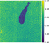 |
Fig. 1 Map of the per-superpixel conversion gain (e− ADU−1) of a flight H2RG detector from the Euclid mission, measured using the standard mean-variance method. The map reveals two distinct regions, a characteristic feature of many H2RG detectors commonly caused by a lack of epoxy between the ROIC and the sensitive layer. Non-negligible gain variations persist even within a single region. |
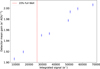 |
Fig. 2 Conversion gain averaged across all pixels of a flight H2RG Euclid detector measured at different integrated signals. The error bars include statistical and systematic errors; the systematic errors are detailed in Sect. 4.2.1. The signal dependence of the gain measurement is clearly visible, with the gain increasing as the integrated signal increases. |
3 Correction of IPC impact on gain measurement
3.1 Interpixel capacitance model
In CMOS APS, the very close proximity of pixels induces a parasitic capacitance between adjacent pixels, known as interpixel capitance (IPC; Moore et al. 2003). These parasitic capacitances cause electrical cross-talk between neighboring pixels, whereby a fraction of the charge generated in a pixel is detected in its neighbors. The classical model that describes the effect of IPC on the signal was well defined in Moore et al. (2004). In this paper, Moore et al. introduced h as the 2D impulse response of a pixel, which describes where the charge generated in the central pixel is detected. Then, the signal Si,j meas detected in a pixel can be described as the convolution of the incoming signal Si,j true onto the detector and the impulse response h, as shown in Eq. (4),
 (4)
(4)
where i and j describe, respectively, the row and column positions of a pixel in the matrix. In an ideal scenario without IPC, the impulse response, defined as a 3 × 3 kernel centered on the considered pixel, should be
 (5)
(5)
Nevertheless, in the presence of IPC, the impulse response can adopt a more complex form. Various expressions of the impulse response with IPC exist, each either neglecting certain terms or assuming horizontal or diagonal symmetry. For example, Moore et al. assume that the diagonals are zero and the cross coefficients are all equivalent, whereas Dudik et al. (2012) assumes that all diagonals are equal to the squared values of the cross coefficients. In order to unify the different expressions, the kernel can be written as
 (6)
(6)
Here, a 3×3 matrix is used. However, if IPC also affects the second neighbors, a 5×5 matrix should be considered. In addition to its effect on the signal, IPC also affects the spatial variance of the signal, thereby biasing the estimation of variance used in the mean-variance method.
3.2 New correction of IPC bias on gain measurement
Because IPC smooths the charge distribution across pixels, it reduces the spatial variance of the signal. As a result, relying on spatial variance to estimate the signal variance could lead to biased conversion gain measurements. Again, based on the definition of the IPC kernel, Moore et al. (2004) developed a method to correct the bias induced by IPC on gain measurement. This method estimates the IPC effect through spatial correlations. However, as previously noted, other factors of spatial correlation, such as persistence, can impede the application of this technique.
However, the framework of Moore et al. remains applicable for defining the impact of IPC on the spatial variance. In that model, the variance estimator in the mean-variance method is given by
 (7)
(7)
Here,  represents the true variance of the signal in ADUs and
  is the zero-lag autocorrelation of the impulse response. Generalizing the work of Moore et al. to Eq. (6), the variance estimator becomes
![Mathematical equation: \mathrm{\hat{var}} = \sigma_S^2 \, \left[ \left(1 - \sum \limits_{i=1}^8 \alpha_i \right)^2 + \sum \limits_{i=1}^8 \alpha_i^2 \right],](/articles/aa/full_html/2026/01/aa56173-25/aa56173-25-eq12.png) (8)
(8)
which may be written in a form similar to Eq. (7) as
 (9)
(9)
A very similar equation can also be obtained with a 5×5 IPC kernel (see Appendix A). Equation (9) illustrates that the impact of IPC on the variance estimator manifests as a multiplier coefficient k, dependent solely on the IPC kernel. Notably, since IPC has been demonstrated to be independent of integrated signals (Ives et al. 2020; Graët et al. 2022), a single coefficient per pixel suffices. Moreover, as IPC does not influence the mean signal estimated via the spatial mean, this coefficient can be applied directly to the biased conversion gain. Thus, taking into account the IPC contribution to the signal variance and incorporating the corresponding variance into Eq. (3), an IPC-free conversion gain can be expressed as
 (10)
(10)
where g^ is the biased gain measured using the classical meanvariance method and g is the “true” gain, namely an IPC-free conversion gain. In the case of a per-superpixel conversion gain, it will be necessary to derive a per-superpixel multiplier coefficient, for instance by using the IPC averaged across the pixels included in the superpixel. Finally, the accurate derivation of this IPC-free gain hinges on the precise measurement of the IPC coefficients αi. Various methodologies for measuring these coefficients are described in Sect. 3.3.
3.3 Validation of the method
To establish the effectiveness of the proposed method to correct for IPC effects on gain measurement, a proper validation process is essential. Figure 3 illustrates a block diagram of the validation pipeline, comparing the results of two distinct methods to obtain an IPC-free gain. The new method, as outlined above, is shown in the lower part of the diagram, while the reference method, previously validated in Graët et al. (2022), is shown in the upper part. In both cases, the IPC coefficients αi must first be determined for each pixel (Fig. 3 - box 2). Several methods, such as singlepixel illumination with 55Fe sources (Fox et al. 2009), analysis of cosmic ray hits (Donlon et al. 2017), or the use of electrical charge generation in hot pixels (Giardino et al. 2012), have been employed for this purpose. However, only methods based on single pixel reset (SPR; see Seshadri et al. 2008) are efficient for measuring the IPC coefficients of each pixel of the sensor.
When using these methods, one should be cautious to measure only IPC and not IPC combined with diffusion, as this model does not account for diffusion. Further studies on the impact of diffusion on spatial correlations are needed to develop a model that accurately integrates these effects. For Euclid ’s IR detectors, a modified SPR technique has been employed.
For the reference method, following the upper line of Fig. 3, these IPC coefficients can be used to directly correct IPC in the raw data to produce an IPC-free conversion gain map. This method is described in Graët et al. (2022) and summarized here. Knowing the IPC kernel k of each pixel (derived from previously measured IPC coefficients) enables the calculation of a corrective kernel, which, when convolved with the IPC kernel, results in the identity kernel. The convolution of each pixel’s raw data with its corresponding corrective kernel then effectively corrects IPC effects (better than 1‰). We therefore applied the latter convolution to all flat-field ramps used in the gain measurement (Fig. 3 - box 3). We then applied the mean-variance method to these “IPC-free” ramps (Fig. 3 - box 4) to produce a conversion gain map that is unbiased by IPC, which serves as our reference gain map. One might question the direct application of this method to measure conversion gain. The need to correct the signal of each pixel in every frame of every ramp dramatically increases the computational time required. For instance, correcting the ramps in this study took as much time as acquiring them, which makes the use of this method as a standard challenging1. Nevertheless, applying it once time provides a useful reference conversion gain map (Fig. 3 - box 5).
The new correction of IPC bias on gain measurements proposed here follows the second line of Fig. 3. First, we applied the mean-variance method to the same raw data set, producing a conversion gain map that initially includes IPC bias (Fig. 3 -box 6). We then used the per-superpixel multiplier coefficients, derived from the αi IPC coefficients as per Eq. (9), to determine an unbiased gain map according to Eq. (10) (Fig. 3 - box 8), resulting in a test conversion gain map (Fig. 3 - box 9).
To assess the efficacy of this new correction, we compared the resulting test map with the reference map. Fig. 4 displays both the comparative map and its histogram, which quantifies the relative difference (%) between the two maps. The spatial mean of the difference is less than 1‱, significantly lower than the gain estimated error (≈1%). This indicates that the two maps are equivalent, validating the use of multiplier coefficients to correct IPC effects on conversion gain measurements. The histogram shows a minor peak at 0.19%, corresponding to superpixels located at the boundary between reference and science pixels2. Similarly, a marginally elevated difference is observed for superpixels along the boundary with the central region of the detector, an area known as the epoxy void (Secroun et al. 2018), which exhibits IPC lower than the rest of the detector. These two regions with larger differences arise from a limitation in the method employed to correct IPC in the raw data, as detailed in Graët et al. (2022). Indeed, this method assumes that the IPC effect of the second neighbor on the first one is the same as the effect of the first neighbor on the central pixel. However, this difference is minimal, and even for affected superpixels, the discrepancy between the two methods is much smaller than the gain measurement error. Importantly, this bias does not originate from the new method itself. Therefore, this new approach is validated and may serve as a standard reference. It offers a considerably fast and light method (nearly instantaneous), necessitating only the prior measurement of IPC coefficients. Moreover, the method is compatible with superpixels of any size or shape - including single pixels - allowing adaptation to the specific spatial behavior of a given detector. In this study, we chose a 16×16 pixel grid as a representative standard.
While this new method provides an easy-to-use tool for correcting the bias created by IPC on conversion gain, the bias arising from the signal dependence of gain measurement remains. In the following section, we present a new derivation of the mean-variance equation that corrects for this dependence.
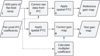 |
Fig. 3 Pipeline for validating the IPC-corrected gain method. The upper part of the diagram (boxes 3 and 4) shows the reference method used to generate the reference map, which is compared with the map produced by the new method shown in the lower part of the diagram (boxes 6-8). |
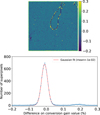 |
Fig. 4 Map (top) and histogram (bottom) of the percentage difference between the conversion gains of the reference and test maps. The mean difference of 1%oo confirms the new correction of the IPC-induced bias in gain measurements using the mean-variance method. |
4 Correction of the nonlinearity impact on gain measurement
Since conversion gain includes several components, as outlined in Sect. 2, which result from the different stages of signal conversion and amplification, nonlinearity may emerge from each of these components. Firstly, the transistors used for voltage signal amplification and buffering are well-known sources of nonlinearity (Hu 2010). This form of nonlinearity is referred to as VV nonlinearity. The second and more substantial source of nonlinearity is attributed to the charge-to-voltage conversion process, or VQ nonlinearity, which is influenced by the varying pn-junction capacitance. Specifically, as photo-generated carriers are collected at the junction, the depletion region narrows, leading to a decrease of the voltage across the junction. Since the junction’s capacitance is dependent on the applied voltage, it will decrease as charges accumulate.
Although they derive from distinct processes, VV and VQ nonlinearities are modeled through a common representation, typically by a polynomial relation between the signal S in ADU and the charge Q in electrons. For instance, Plazas et al. (2017) and Hirata & Choi (2019) use a second-order polynomial model of the pixel response as illustrated in Eq. (11),
 (11)
(11)
In this equation, the coefficient β, expressed in units of e−1, encompasses both V/V and V/Q nonlinearities. These polynomial models are also implicitly used by different missions employing CMOS APS (Kubik et al. 2014; Canipe et al. 2017) to correct the impact of nonlinearity on flux estimation. Specifically, the flux in ADUs per second is assumed to follow a polynomial model. Because the photon flux and the conversion from photons to electrons (QE) are constant, the polynomial nature of flux in ADUs per second is presumed to arise from the conversion of electrons to ADUs. For the correction of flux nonlinearity, depending on the mission, the order of the polynomial is often increased to achieve a better fit with the data. However, even though this polynomial flux correction has been commonly used, the mean-variance equation is still derived assuming a linear pixel response. To properly use the mean-variance curve to estimate the conversion gain, this equation needs to be modified. In the following section, we develop the mean-variance calculation that incorporates nonlinear models and then apply it to measure the conversion gain.
4.1 Nonlinear mean variance method
Nonlinear models can be based on polynomials of any order. Hereafter, we consider polynomials of second and third order.
4.1.1 Second-order polynomial model
First, we consider the second-order polynomial pixel response. Based on Eq. (11), assuming that g, Q, and β are independent (which also implies that g is constant), and including the readout noise σR as in Eq. (3), the error propagation formula can be written as
 (12)
(12)
where  is the variance of the measured signal. Assuming that, for one pixel, the variances of g and β are negligible, and knowing that the accumulated charge Q follows a Poisson distribution, it follows that
 (13)
(13)
Rearranging the terms yields
 (14)
(14)
and combining Eq. (11) squared with Eq. (14) yields
 (15)
(15)
As mentioned previously, several missions apply polynomial fitting to their ramp data to correct for the impact of nonlinearity on flux measurements. This method also allows an estimate of β through the second-order coefficient. According to recent estimates by the Euclid characterization team, β is on the order of −5 × 10⁻⁷e−1 (Fourmanoit 2021). Similar estimates have been obtained by Plazas et al. (2017) and Hirata & Choi (2019). Therefore, with such a value for β and an integrated signal lower than 70 ke−, the ratio of the second to the third term in Eq. (15) exceeds 80. Therefore, the third term can be neglected. Equation (15) then simplifies to
 (16)
(16)
Equation (16) forms the basis of a new nonlinear mean-variance method that enables the derivation of the conversion gain g in the presence of nonlinearities. In practice, plotting the variance as a function of the mean signal for a pixel and fitting it with a second-order polynomial (rather than a first order polynomial) allows the derivation of the conversion gain as the first order coefficient. The nonlinearity coefficient β may be obtained as that of the second order. This new approach is denoted below as the NL2 mean-variance.
4.1.2 Third-order polynomial model
The same calculation applies using a third-order polynomial model for the pixel response, as given in Eq. (17),
 (17)
(17)
with γ is the nonlinear third-order coefficient in e−2. Using the same assumptions as in Sect. 4.1.1, the variance of the signal can be written as
 (18)
(18)
Fitting the mean-variance curve with a third-order polynomial again allows the determination of the gain from the first-order coefficient. We denote this approach as the NL3 mean-variance. In the following section, we apply and validate the standard mean-variance method, together with the two nonlinear NL2 and NL3 adaptations introduced here, using Euclid characterization data to compute a gain corrected for nonlinearity.
4.2 Validation of the nonlinear mean-variance method
To assess and compare the gain values obtained from the three different mean-variance modeling approaches introduced here, namely linear, NL2, and NL3, we implemented two distinct strategies. First, we examined and compared the dependence of gain measurements on integrated signal using the three methods. This comparison determined whether the new methods are compatible with the hypothesis that gain is independent of integrated signal. Second, statistical tests provided indications of whether the new models yield a significantly improved assessment of gain.
4.2.1 Gain variations with integrated signal
To evaluate the efficiency of the three methods, we applied them to the same data set referenced in Sect. 3, fitting the mean-variance curve with orthogonal polynomials. As mentioned earlier, this dataset consists of flat-field pairs of ramps acquired under various fluxes with constant integration time. By dividing the data set into smaller subsets with the same integrated signal and measuring the conversion gain for each subset, the influence of the integrated signal on gain measurement can be investigated. In Fig. 5, the three mean-variance methods are applied to these subsets and the mean detector gain is plotted against the integrated signal in electrons (estimated from LED calibration). Gain values can be averaged across the detector due to the verified uniformity of the pixel response nonlinearity. Because the gain is averaged across the entire detector, the statistical error is very low, with error bars dominated by systematic error. This systematic error arises from flux-dependent effects, such as persistence, leading to variations in gain measurement for pairs of ramps acquired under different fluxes, even with identical integrated signal.
As previously seen in Fig. 2, the gain measured with the classical linear mean-variance equation (blue in Fig. 5) clearly increases with the integrated signal, which is incompatible with the hypothesis that gain is independent of integrated signal. This behavior may be attributed, at least in part, to some nonlinearity related to the reduction of the junction capacitance. For the two nonlinear mean-variance methods, NL2 and NL3, the detector’s mean coefficient β is measured at (−4.2 ± 0.1) × 10−7 e−1 and (−5.6 ± 0.6) × 10−7 e−1, respectively. In addition to validating the assumption used to derive Eqs. (15) and (18), both values are consistent with the Euclid characterization team’s estimation of β. Using the NL2 mean-variance model (red in Fig. 5), for integrated signal levels lower than 50 ke−, the measured gain aligns with the expectation of a constant gain. At higher integrated signal levels, however, the gain increases with integrated signal once more, indicating that a second-order polynomial is insufficient to fully capture the nonlinearity of the meanvariance curve. In contrast, the gain measured using the NL3 mean-variance model (green in Fig. 5) remains consistent with a constant gain, within uncertainties, across all integrated signal levels between 10 and 70ke− (≈60% of the full well capacity). These findings strongly indicate that a third-order polynomial is best suited to model the mean-variance curve accurately and to derive a truly constant gain value. Using the NL3 meanvariance model instead of the linear one corrects a mean bias of approximately 2.5% in gain measurement.
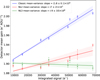 |
Fig. 5 Conversion gain averaged across all pixels of a flight H2RG Euclid detector measured at different integrated signals using linear, NL2, and NL3 mean-variance methods. For each method, a linear regression and its 1-sigma confidence interval are plotted. Only the NL3 mean-variance method is consistent with the hypothesis that the gain remains constant with integrated signal. The mean gain measurement is 2.5% lower when measured with the NL3 mean-variance method compared to the linear method. |
4.2.2 Complementary validation with statistical tests
Conclusively validation of the NL3 mean-variance method requires a strict statistical analysis. We conducted this analysis using a partial F-test. This test is designed to assess the significance of adding or removing variables from a regression model. First, it is necessary to define the null hypothesis to be tested. In this context, the null hypothesis assumes that the model with fewer variables fits the mean-variance curve as effectively as the models with additional variables. Should the null hypothesis not be rejected, it implies that the model with more variables does not offer a significantly improved fit.
To evaluate the null hypothesis, the partial F-test relies on comparing the sum of square residuals (SSR) between the two considered model fits. Hereafter, SSR1 represents the SSR for the models with fewer variables, while SSR2 denotes the SSR for the alternative model. The respective numbers of parameters for these models are denoted as p1 and p2 and n is the number of points used to fit the model (the number of frames in our study). Under the null hypothesis, the ratio defined in Eq. (19) follows a Fisher (F) distribution with degrees of freedom (p2 - p1, n - p2). For each of the mean curve variance used to measure the gain, the SSR from the fits with the two models under comparison, using Eq. (19),
 (19)
(19)
allows for the calculation of the fvalue. To refute the null hypothesis, we computed the cumulative distribution function of an F distribution with degrees of freedom (p2 - p1, n - p2), evaluated at the fvalue. If the probability P(F ≤ fvalue) > 1 - α for a given significance level α, then the null hypothesis can be dismissed and the test is successful. A successful test leads to the conclusion that the model with additional variables provides a better fit than that with fewer variables. A typical significance level is set to 0.05 (probability of 95%), but when multiple comparisons are made, the probability of incorrectly rejecting the null hypothesis increases. In this case, since an F-test is performed for each mean-variance curve used to measure a gain value, the significance level must be adjusted accordingly. To address this, we applied a Bonferroni correction to the significance level, given by  , where M is the number of comparisons.
We conducted two partial F-tests: one to assess whether the NL2 mean-variance model outperforms the linear model, and another to determine whether the NL3 mean-variance model provides a better fit than the NL2 model. As these evaluations were performed for all mean-variance curves, the outcome for each curve is whether or not the F-test is successful. Specifically, the percentage of mean-variance curves that pass the test is computed for each superpixel, and their distribution is represented in Fig. 6. If more than half of the mean-variance curves pass the test, the model with more variables is validated.
As observed, for all superpixels, more than 60% of the meanvariance curves are represented more accurately by the NL2 model than by the linear model. Moreover, for more than 50% of the mean-variance curves across all superpixels, the NL3 model successfully passes the test. This confirms that the NL3 mean-variance model is preferable for measuring the conversion gain of the Euclid IR detectors. Investigations have begun into the use of a fourth-order model; however, deriving the variance formulas for such models becomes extremely complex, and for the Euclid detector, the fourth order is dominated by noise. Therefore, for now, the NL3 mean-variance model remains the best-suited method for measuring a conversion gain independent of integrated signal.
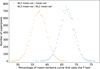 |
Fig. 6 Distribution across superpixels of the percentage of meanvariance curves that pass the F-test for two comparisons: NL2 mean-var vs. standard mean-var and NL3 mean-var vs. NL2 mean-var. For a superpixel, if more than 50% of the mean-variance curve passes the test, the new model is considered validated. |
5 Conclusions
This study presents an innovative method for accurately measuring the conversion gain in CMOS active pixel sensors, with a particular focus on correcting the biases created by both IPC and nonlinearity. The derivation of a new mean-variance equation, based on a polynomial description of the pixel response, allows for the definition of a nonlinear mean-variance method that accounts for detector nonlinearity. Furthermore, to correct the bias introduced by IPC in gain measurements, the method uses only a multiplier coefficient calculated from per-pixel IPC coefficients, making it both faster and more efficient than typical methods. Applied to on-ground characterization data from a Euclid infrared detector, this method underwent rigorous validation, demonstrating its effectiveness in correcting IPC bias and measuring a gain independent of integrated signal. Because it allows per-superpixel measurements of conversion gain decorrelated from IPC and nonlinearity, and requires only knowledge of IPC coefficients, this new method, applicable to any CMOS APS, can be used as a new reference.
Acknowledgements
This work was developed within the frame of a CNES-CNRS funded Phd thesis. The Euclid Consortium acknowledges the European Space Agency and a number of agencies and institutes that have supported the development of Euclid, in particular the Agenzia Spaziale Italiana, the Austrian Forschungsförderungsgesellschaft funded through BMK, the Belgian Science Policy, the Canadian Euclid Consortium, the Deutsches Zentrum für Luft- und Raumfahrt, the DTU Space and the Niels Bohr Institute in Denmark, the French Centre National d’Etudes Spatiales, the Fundaçâo para a Ciência e a Tecnologia, the Hungarian Academy of Sciences, the Ministerio de Ciencia, Innovación y Universidades, the National Aeronautics and Space Administration, the National Astronomical Observatory of Japan, the Netherlandse Onderzoekschool Voor Astronomie, the Norwegian Space Agency, the Research Council of Finland, the Romanian Space Agency, the State Secretariat for Education, Research, and Innovation (SERI) at the Swiss Space Office (SSO), and the United Kingdom Space Agency. A complete and detailed list is available on the Euclid web site (www.euclid-ec.org).
References
- Barbier, R., Buton, C., Clemens, J.-C., et al. 2018, SPIE, 10709, 173 [Google Scholar]
- Beecken, B. P., & Fossum, E. R. 1996, Appl. Opt., 35, 3471 [Google Scholar]
- Bezawada, N., Ives, D., & Woodhouse, G. 2004, SPIE, 5499, 23 [Google Scholar]
- Bezawada, N., Ives, D., & Atkinson, D. 2007, SPIE, 6690, 669005 [Google Scholar]
- Bezawada, N., George, E., Ives, D., et al. 2023, Astron. Nachr., 344, e20230061 [Google Scholar]
- Canipe, A. M., Robberto, M., & Hilbert, B. 2017, AAS Meeting Abstracts, 230, 114.02 [Google Scholar]
- Cisneros-González, M. E., Bolsée, D., Pereira, N., et al. 2020, SPIE, 11443, 271 [Google Scholar]
- Claveau, C.-A., Bottom, M., Jacobson, S., et al. 2022, SPIE, 12191, 121910Z [Google Scholar]
- Donlon, K., Ninkov, Z., Baum, S., & Cheng, L. 2017, Opt. Eng., 56, 024103 [Google Scholar]
- Dudik, R. P., Jordan, M., Dorland, B. N., et al. 2012, Appl. Opt., 51, 2877 [Google Scholar]
- Euclid Collaboration (Jahnke, K., et al.) 2025a, A&A, 697, A3 [Google Scholar]
- Euclid Collaboration (Mellier, Y., et al.) 2025b, A&A, 697, A1 [Google Scholar]
- Finger, G., Beletic, J., Dorn, R., et al. 2005, Exp. Astron., 19, 135 [Google Scholar]
- Fossum, E. 1997, IEEE Trans. Electron Devices, 44, 1689 [Google Scholar]
- Fourmanoit, N. 2021, Euclid Internal Documentation, Technical report [Google Scholar]
- Fox, O., Waczynski, A., Wen, Y., et al. 2009, PASP, 121, 743 [Google Scholar]
- Fraser, G. W., Abbey, A. F., Holland, A., et al. 1994, Nucl. Instrum. Methods Phys. Res. A, 350, 368 [Google Scholar]
- Giardino, G., Sirianni, M., Birkmann, S. M., et al. 2012, SPIE, 8453, 84531T [Google Scholar]
- Graët, J. L., Secroun, A., Barbier, R., et al. 2022, SPIE, 12191, 562 [Google Scholar]
- Gravrand, O., Lobre, C., Santailler, J.-L., et al. 2022, SPIE, 12107, 1210706 [Google Scholar]
- Greffe, T., Smith, R., Sherman, M., et al. 2022, SPIE, 12191, 72 [Google Scholar]
- Guellec, F., Boulade, O., Cervera, C., et al. 2017, SPIE Conf. Ser., 10563, 105630K [Google Scholar]
- Hendrickson, A., & Haefner, D. P. 2023, SPIE, 12533, 253 [Google Scholar]
- Hirata, C. M., & Choi, A. 2019, PASP, 132, 014501 [Google Scholar]
- Hu, C. 2010, Modern Semiconductor Devices for Integrated Circuits (New Jersy, NJ: Prentice Hall Upper Saddle River), 2 [Google Scholar]
- Ives, D., Alvarez, D., Bezawada, N., George, E., & Serra, B. 2020, SPIE, 11454, 67 [Google Scholar]
- Janesick, J. R. 2001, Scientific Charge-Coupled Devices (USA: SPIE) [Google Scholar]
- Janesick, J., Andrews, J. T., & Elliott, T. 2006, SPIE, 6276, 208 [Google Scholar]
- Kubik, B., Barbier, R., Castera, A., et al. 2014, SPIE, 9154, 91541Q [Google Scholar]
- McCullough, P. 2008, Inter-Pixel Capacitance: Prospects for Deconvolution, Technical report [Google Scholar]
- Moore, A. C., Ninkov, Z., Burley, G. S., et al. 2003, SPIE, 5017, 240 [Google Scholar]
- Moore, A. C., Ninkov, Z., & Forrest, W. J. 2004, SPIE Conf. Ser., 5167, 204 [NASA ADS] [Google Scholar]
- Moore, A. C., Ninkov, Z., & Forrest, W. J. 2006, Opt. Eng., 45, 076402 [Google Scholar]
- Mortara, L., & Fowler, A. 1981, SPIE, 290, 28 [Google Scholar]
- Mosby, G., Rauscher, B. J., Bennett, C., et al. 2020, J. Astron. Telesc. Instrum. Syst., 6, 046001 [Google Scholar]
- Pain, B., & Hancock, B. R. 2003, SPIE, 5017, 94 [Google Scholar]
- Pichon, T., Schwartz, V., Gougeon, A., et al. 2022, SPIE, 12191, 121911P [Google Scholar]
- Plazas, A., Shapiro, C., Smith, R., Rhodes, J., & Huff, E. 2017, J. Instrum., 12, C04009 [NASA ADS] [CrossRef] [Google Scholar]
- Rauscher, B. J., Fox, O., Ferruit, P., et al. 2007, PASP, 119, 768 [NASA ADS] [CrossRef] [Google Scholar]
- Rauscher, B. J., Boehm, N., Cagiano, S., et al. 2014, PASP, 126, 739 [NASA ADS] [Google Scholar]
- Rogalski, A. 2011, Infrared Phys. Technol., 54, 136 [Google Scholar]
- Secroun, A., Serra, B., Clémens, J. C., et al. 2016, SPIE, 9915, 649 [Google Scholar]
- Secroun, A., Barbier, R., Buton, C., et al. 2018, SPIE, 10709, 513 [Google Scholar]
- Seshadri, S., Cole, D. M., Hancock, B. R., & Smith, R. M. 2008, SPIE, 7021, 54 [Google Scholar]
- Smith, R. M., Zavodny, M., Rahmer, G., & Bonati, M. 2008, SPIE, 7021, 70210J [Google Scholar]
- Soman, M., Stefanov, K., Weatherill, D., et al. 2015, J. Instrum., 10, C02012 [Google Scholar]
Calculation were performed using 22 Intel (R) Xeon(R) CPU E5-2640 v3 at 2.60 GHz.
For H2RG detectors, the 2048×2048 matrix is divided into “science” pixels, the actual sensitive pixels, and “reference” pixels, which form a frame of four external lines and columns of nonsensitive pixels that surround the science pixels and that are usually used for noise correction.
Appendix A Gain corrective coefficient for 5x5 IPC kernel
If the IPC between a pixel and his second neighbors is not negligible, the impulse response of a pixel needs to be a 5×5 kernel as
 (A.1)
(A.1)
Then, the corrective coefficient of Eq. (9) becomes :
 (A.2)
(A.2)
 (A.3)
(A.3)
 (A.4)
(A.4)
All Figures
|
Fig. 1 Map of the per-superpixel conversion gain (e− ADU−1) of a flight H2RG detector from the Euclid mission, measured using the standard mean-variance method. The map reveals two distinct regions, a characteristic feature of many H2RG detectors commonly caused by a lack of epoxy between the ROIC and the sensitive layer. Non-negligible gain variations persist even within a single region. |
| In the text | |
|
Fig. 2 Conversion gain averaged across all pixels of a flight H2RG Euclid detector measured at different integrated signals. The error bars include statistical and systematic errors; the systematic errors are detailed in Sect. 4.2.1. The signal dependence of the gain measurement is clearly visible, with the gain increasing as the integrated signal increases. |
| In the text | |
|
Fig. 3 Pipeline for validating the IPC-corrected gain method. The upper part of the diagram (boxes 3 and 4) shows the reference method used to generate the reference map, which is compared with the map produced by the new method shown in the lower part of the diagram (boxes 6-8). |
| In the text | |
|
Fig. 4 Map (top) and histogram (bottom) of the percentage difference between the conversion gains of the reference and test maps. The mean difference of 1%oo confirms the new correction of the IPC-induced bias in gain measurements using the mean-variance method. |
| In the text | |
|
Fig. 5 Conversion gain averaged across all pixels of a flight H2RG Euclid detector measured at different integrated signals using linear, NL2, and NL3 mean-variance methods. For each method, a linear regression and its 1-sigma confidence interval are plotted. Only the NL3 mean-variance method is consistent with the hypothesis that the gain remains constant with integrated signal. The mean gain measurement is 2.5% lower when measured with the NL3 mean-variance method compared to the linear method. |
| In the text | |
|
Fig. 6 Distribution across superpixels of the percentage of meanvariance curves that pass the F-test for two comparisons: NL2 mean-var vs. standard mean-var and NL3 mean-var vs. NL2 mean-var. For a superpixel, if more than 50% of the mean-variance curve passes the test, the new model is considered validated. |
| In the text | |
Current usage metrics show cumulative count of Article Views (full-text article views including HTML views, PDF and ePub downloads, according to the available data) and Abstracts Views on Vision4Press platform.
Data correspond to usage on the plateform after 2015. The current usage metrics is available 48-96 hours after online publication and is updated daily on week days.
Initial download of the metrics may take a while.