| Issue |
A&A
Volume 705, January 2026
|
|
|---|---|---|
| Article Number | A46 | |
| Number of page(s) | 18 | |
| Section | Planets, planetary systems, and small bodies | |
| DOI | https://doi.org/10.1051/0004-6361/202556827 | |
| Published online | 07 January 2026 | |
Gaia and IRTF abundance of A-type main-belt asteroids
1
Université Côte d’Azur, CNRS–Lagrange, Observatoire de la Côte d’Azur,
CS
34229 – 06304 NICE
Cedex 4,
France
2
University of Leicester, School of Physics and Astronomy,
University Road,
LE1 7RH
Leicester,
UK
3
INAF-IAPS, Institute for Space Astrophysics and Planetology,
Rome,
Italy
4
Eureka Scientific,
Oakland,
CA
94602,
USA
5
Osservatorio Astronomico di Roma,
Via Frascati 33,
00078
Monte Porzio Catone,
Italy
★ Corresponding authors: This email address is being protected from spambots. You need JavaScript enabled to view it.
Received:
11
August
2025
Accepted:
24
October
2025
Abstract
Context. The so-called missing-mantle problem is a long-standing issue in planetary science. It states that olivine-rich asteroids should be abundant in the main belt, while this is observationally found not to be the case by dedicated surveys. Conversely, olivine-rich asteroids appear to be more abundant among near-Earth asteroids than those surveys would suggest.
Aims. We aim to provide a revised estimate of the abundance of A-type (olivine-rich) asteroids in the main belt by combining taxonomic classifications from Gaia Data Release 3 reflectance spectra with ground-based near-infrared observations from NASA’s IRTF.
Methods. We performed a principal component analysis on Gaia Data Release 3 visible-light reflectance spectra to identify A-type candidates and confirmed a subset of these using near-infrared spectroscopy from the IRTF. We combined our observations with data from the literature to compute the A-type probability distribution as a function of the principal components of Gaia reflectance spectra. This probability distribution was then used to estimate the abundance of A-type asteroids in the main belt and its sub-populations as a function of heliocentric distance. We also examined the distribution of A-type asteroids among known collisional families.
Results. We found that the abundance of A types in the main belt is (2.00 ± 0.15)%, which is significantly higher than previous estimates for the same region. Our analysis also shows that some collisional families, such as those of Vesta and Flora, have above-average A-type fractions, whereas others, such as Themis and Hygiea, exhibit negligible abundance.
Conclusions. Our results support the idea that olivine-rich material is more widespread than previously thought. In particular, the high A-type abundance in the Flora family is consistent with the hypothesis of a second differentiated parent body in the inner main belt, beyond Vesta. This work provides new observational constraints on the missing-mantle problem and the distribution of differentiated material in the asteroid main belt. In particular, our results deepen the compositional diversity observed in the inner main belt and have important implications for our understanding of early Solar System differentiation processes.
Key words: techniques: spectroscopic / astronomical databases: miscellaneous / minor planets, asteroids: general
© The Authors 2026
 Open Access article, published by EDP Sciences, under the terms of the Creative Commons Attribution License (https://creativecommons.org/licenses/by/4.0), which permits unrestricted use, distribution, and reproduction in any medium, provided the original work is properly cited.
This article is published in open access under the Subscribe to Open model. This email address is being protected from spambots. You need JavaScript enabled to view it. to support open access publication.
1 Introduction
It is well understood that main-belt asteroids are remnants of the planetesimals that escaped merging collisions to form the terrestrial planets (Morbidelli et al. 2025) and the dynamical ejection out of our Solar System (planetesimals are the so-called first ~100 km sized bodies that accreted from the dust of our protoplanetary disc, as reviewed by Klahr et al. 2022).
Mutual collisions between asteroids created, continuously over time (Brož et al. 2013; Spoto et al. 2015), families of fragments (Nesvorný et al. 2015; Delbo’ et al. 2017; Delbo et al. 2019; Ferrone et al. 2023; Nesvorný et al. 2024) that we can still identify today. Family members dominate today’s main belt asteroid population (Delbo’ et al. 2017; Dermott et al. 2018; Ferrone et al. 2023) and are recognised as the main sources of meteorites (Greenwood et al. 2020; Avdellidou et al. 2022; Brož et al. 2024a,b; Marsset et al. 2024). Hence, meteorites and samples returned from asteroids (Lauretta et al. 2024) allow us to probe the materials that constituted the planetesimals (Bourdelle de Micas et al. 2022) and to infer information about the dynamical processes that sculpted our Solar System (see e.g. Avdellidou et al. 2024).
A fraction of meteorites have compositions consistent with origins from differentiated planetesimals (Burbine et al. 2002, in particular their Table 2). These are the bodies that underwent processes of internal heating strong enough to cause their materials, originally mixed together as undifferentiated (or chondritic), to separate into distinct layers, i.e. a core, a mantle, and a crust (Neumann et al. 2012 and references therein). This internal heating is thought to have originated from the decay of radioactive elements (mainly 26Al; see e.g. Urey 1955, but also 60Fe) that were spread over the protoplanetary disc (MacPherson et al. 1995) and therefore accreted into the early planetesimals.
In a fully differentiated object, the core is made of ironnickel metal, the mantle is constituted of igneous silicates, such as olivine – which is commonly found in mafic and ultramafic igneous rocks and is composed of magnesium and iron silicate (Fe, Mg)2SiO4 – and the crust is also composed of igneous rocks, such as basalt (Weiss & Elkins-Tanton 2013). The latter may have formed from the rapid cooling of lava material exposed to space. Partially differentiated planetesimals would still preserve a crust of undifferentiated chondritic materials at various metamorphic grades (see Fig. 2 of Weiss & Elkins-Tanton 2013) overlying an olivine rich mantle and an iron core. The type of differentiation is primarily controlled by the onset and stop of the heating process (see Fig. 3 of Weiss & Elkins-Tanton 2013). The former is related to the epoch of planetesimal accretion, and the latter is mostly controlled by the planetesimal size and thermal conductivity. The various degrees of differentiation explain the diversity of meteorites, which ranges from undifferentiated chondrites to metallic meteorites, including those with varying degrees of metamorphism.
Different types of meteorites have successfully been linked to different asteroid spectroscopic types by studying the features of their spectra, such as ordinary chondrites (Brož et al. 2024b; Marsset et al. 2024, and references therein), basaltic meteorites (i.e. crustal; see Moskovitz et al. 2008; Solontoi et al. 2012; Leith et al. 2017), enstatite meteorites (Avdellidou et al. 2022), carbonaceous chondrites (Brož et al. 2024a), and metallic meteorites (Harris & Drube 2014; Avdellidou et al. 2025). However, it has been claimed that there is a shortage of olivine-dominated mantle material – a tracer of differentiation – in the main belt (DeMeo et al. 2019). This conundrum is known as the missing-mantle problem or the great dunite shortage, which is a long-standing issue in planetary science (Chapman 1986; Bell et al. 1989); that is, olivine-rich asteroids should be abundant in the main belt, while this is observationally found not to be the case (see also DeMeo et al. 2019).
Olivine-rich asteroids are typically identified as having spectroscopic A-type classes in the Bus and Binzel (Bus & Binzel 2002) and/or in the Bus-DeMeo (DeMeo et al. 2009) taxonomies. The latter is more reliable due to its extension in the near-infrared (NIR), which is a very good diagnostic for this class. Namely, A types have very high reflectance in the NIR with no or a very weak 2 μm absorption band, a characterisation via reference spectra with very red slopes at wavelengths ≲0.7 μm, and a strong absorption feature centred slightly longwards of 1 μm (e.g. Bus & Binzel 2002; DeMeo et al. 2009; Sanchez et al. 2014; DeMeo et al. 2019). Moreover, A-types have moderate to high geometric visible albedo values (![Mathematical equation: $\[p_{\mathrm{V}}\text{=}0.26_{-0.08}^{+0.11}\]$](/articles/aa/full_html/2026/01/aa56827-25/aa56827-25-eq1.png) ), as we show in Sect. 5.1. A types show the closest spectroscopic similarities to brachinite and pallasite meteorites (Burbine & Binzel 2002). Since these meteorites originated in the mantle and in the core-mantle boundary of differentiated planetesimals (Benedix et al. 2014), it is reasonable to assume that A-type asteroids could represent fragments from these layers of a differentiated planetesimal.
), as we show in Sect. 5.1. A types show the closest spectroscopic similarities to brachinite and pallasite meteorites (Burbine & Binzel 2002). Since these meteorites originated in the mantle and in the core-mantle boundary of differentiated planetesimals (Benedix et al. 2014), it is reasonable to assume that A-type asteroids could represent fragments from these layers of a differentiated planetesimal.
The most recent survey of A types in the main belt (DeMeo et al. 2019) made use of the Sloan Digital Sky Survey (SDSS) Moving Object Catalog visible (VIS) photometric data to select a number of candidate A-type asteroids; then, the NIR spectroscopy of the candidates by means of SpeX on the NASA Infrared Telescope Facility (IRTF) and the Folded-port InfraRed Echellette (FIRE) on the Magellan Telescope was performed to confirm their A-type classes. By multiplying the confirmation rate and the number of candidates compared to the total asteroid population, this survey found that A types only represent 0.16% of the main-belt asteroids with sizes ≥2 km. These results led us to conclude that the missing-mantle problem is a fact and that asteroid differentiation was not as widespread as previously thought (DeMeo et al. 2019). Moreover, it was found that A types are evenly distributed throughout the main belt, even detected at the distance of the Cybele region, and have no statistically significant concentration in any asteroid collisional family. However, Galinier et al. (2024) discovered that the outer main-belt family (36256) 1999 XT17 presents a prominence of A-type objects, thus ruling out the hypothesis of DeMeo et al. (2019) that A-types have no statistically significant concentration in any collisional family. In addition to (36256) 1999 XT17, Galinier et al. (2024) indicated other collisional families potentially having abundance of A types.
Marsset et al. (2022) combined NIR spectra of near-Earth objects (NEOs) collected as part of the MIT-Hawaii NEO Spectroscopic Survey with data retrieved from Binzel et al. (2019) to derive the intrinsic compositional distribution of the overall NEO population. Their bias-corrected distribution shows that the A-types account for the 0.1–0.5% of the sample coming from each different NEO source region.
Moreover, Sergeyev et al. (2023) used spectrophotometric data from the SDSS and SkyMapper surveys and reported that A-type asteroids constitute 2.5±0.2% of the near-Earth asteroid (NEA) population. This fraction is more than 15 times higher than the A-type abundance derived by DeMeo et al. (2019) for the main asteroid belt. Sergeyev et al. (2023) also find that A types show a higher number density in the region between the orbit of Mars and Jupiter’s 4:1 mean motion resonance, which is predominantly occupied by the Hungaria asteroid population. These results suggested a potential link between Hungaria asteroids and A-type NEAs.
Similar findings were reported by Devogèle et al. (2019). They estimated that A types account for 3.8±1.3% of the NEA population. They identified an excess of A-types at semi-major axes around 1.6 au, which corresponds to the 1:2 mean motion resonance with Earth. This resonance likely facilitates the transfer of Hungaria family asteroids into the NEA population. Further supporting these observations, Lucas et al. (2019) conducted a spectroscopic survey of the Hungaria region and found an A-type fraction of 1.5%. Furthermore, Popescu et al. (2018) identified an abundance of 5.4% of A-types in a sample of 147 NEAs with diameters less than 300 m, which were surveyed in the visible wavelength range. Similarly, Perna et al. (2018) found an abundance of A types of 5.48% among 146 NEAs based on ground-based observations also in the visible range. However, we should treat A-type classification based only on the VIS spectrum with caution: DeMeo et al. (2019) showed that their typical A-type confirmation rate using NIR spectroscopy is about 1/3 of the potential A types identified from VIS spectrophotometry (SDSS). In addition, care should be taken when directly comparing the main-belt surveys with the NEO ones, because they are potentially affected by different observing biases. For instance, in the case of NEOs, by focusing on targets on specific orbits (e.g. low-Δv), a bias in favour of objects coming from specific NEO source regions in the main belt may be applied. This can result in samples that are not representative of the overall main-belt population. Moreover, NEO and main-belt surveys probe different size ranges, which could affect the inferred A-type fractions.
All the results presented above indicate that the missingmantle problem might need a review in the light of new astronomical data. Gaia Data Release 3 (Gaia DR3) provided to the community with an unprecedented dataset of more than 60,000 asteroid visible reflectance spectra (Gaia Collaboration 2023). Such a dataset can be used to perform new searches for the missing olivine in the main belt (Galinier et al. 2024). Namely, we used Gaia DR3 data to inform target selection for a spectroscopic survey of main-belt asteroids in the NIR (using NASA’s IRTF) that we combined with existing literature data to test Gaia DR3 predictions for A-type asteroids.
In Sect. 2, we present the Gaia DR3 dataset. In Sect. 3, we provide the target selection for the NIR observations. In Sect. 4, we state the analysis and results, which we then discuss in Sect. 5.
2 Data and target selection
We made use of VIS reflectance spectra that were derived from asteroid spectroscopic observations obtained by the Gaia space mission of the European Space Agency (ESA) between 5 August 2014 and 28 May 2017 and were published as part of Gaia DR3 (Gaia Collaboration 2023; Tanga et al. 2023). It contains 60,518 Solar System small bodies, mostly main belt asteroids. Each asteroid has an associated unique mean reflectance spectrum obtained by averaging several epoch spectra, which span the VIS wavelength range between 0.374 and 1.034 μm. All mean reflectance spectra are expressed by the same 16 discrete wavelength bands. A ‘reflectance_spectrum_flag’ (RSF) is associated with each band, signalling whether the band reflectance value and its uncertainty are validated (RSF=0), suspected to be of poor quality (RSF=1), or not good (RSF=2). There is evidence that Gaia DR3 reflectance spectra overestimate the reflectance values in the reddest bands (Gaia Collaboration 2023; Galinier et al. 2023, 2024), which, however, does not appear to cause problems in the identification of A types (Galinier et al. 2024). The two bluest bands are also often affected by large uncertainties and have RSF>0 (Gaia Collaboration 2023; Delbo et al. 2023). Tinaut-Ruano et al. (2023) showed that the set of solar analogues adopted by Gaia Collaboration (2023) yields asteroid reflectances with systematically redder spectral slopes at wavelengths shorter than 0.55 μm compared to using Hyades 64 alone, the latter being considered the most Sun-like in the near-ultraviolet. They proposed a correction for reflectance bands shorter than 0.55 μm. We do not apply this correction here, because it does not affect A-type identification; this relies primarily on wavelengths longer than 0.55 μm.
Our aim was to identify A types in the Gaia DR3 dataset. One could do so by first performing a classification of the Gaia DR3 spectra and then identifying the objects that belong to the A class. However, because of the systematic effects described above, we preferred to follow another established method. We carried out a principal component analysis (PCA) of the Gaia DR3 reflectance spectra, which represent a linear transformation from the reflectance space to another coordinate space where the greatest variance lies along the first axis (principal component), the second greatest variance along the second axis, and so on, effectively capturing the most important patterns in the data. Clusters of points in the PCA space are expected to correspond to taxonomic classes (Appendix D). This is similar to the approach used by DeMeo et al. (2019) for their identification of potential A types in the SDSS and by Choi et al. (2023) for their taxonomic classification using the KMTNet multi-band photometry.
Before presenting our methods, we describe the data selection procedure: (i) we applied the PCA only to Gaia DR3 reflectance spectra with S/N > 50 (where the S/N is calculated as in Gaia Collaboration 2023) to ensure that the PCA transformation was not biased by noisier data. This resulted in the definition of the PCA transformation on 9,332 objects, which we then applied to the whole DR3 dataset, regardless of the S/N. We also tested lower S/N thresholds – for example, 30 and 20; corresponding to 20,866 and 36,551 asteroids, respectively – and found that the results did not change appreciably. We excluded the two reddest and two bluest wavelength bands in the PCA fit and discarded reflectance bands with RSF > 0. We retained five principal components in total, but found that the first and second components, hereafter referred to as PC1 and PC2, respectively, carry most of the variance of the data. Namely, we found that the variance of the PC1–5 components are, respectively, 0.057, 0.017, 0.007, 0.004, and 0.004. As expected, the position of asteroids in the PC1–PC2 plot is diagnostic of their compositional spectral class (Fig. D.1).
Next, we needed a ground-truth sample of A types with Gaia DR3 data to locate them in the PCA space. NIR spectroscopy is the most robust A-type identification method because it is sensitive to the distinguishing features of this class, as explained in the introduction. Hence, we retrieved all main-belt asteroids from the literature that were classified A types from both VIS and NIR spectroscopy (VIS+NIR) and have a corresponding Gaia DR3 reflectance spectrum. Our search resulted in 44 asteroids (Table B.1), which is a small set compared to the 1,755 asteroids that have spectral classes derived from VIS and NIR spectroscopy (A-type and non-A-type). The PCA was calculated on Gaia DR3 with an S/N>50, but asteroids were retrieved from literature or selected for NIR observations regardless of the S/N of their Gaia DR3 reflectance spectrum. The PC1 and PC2 values of A types revealed that they are preferentially located at large PC1 and negative PC2 values (Fig. 1), adjacent to the S-complex cluster (Appendix D). The latter is centred at PC1 ~0.17 and PC2~ −0.06, as can be seen in the S-type plot of Fig. D.1.
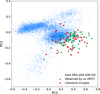 |
Fig. 1 PC1 versus PC2 plot of main-belt asteroid reflectance spectra from the Gaia DR3 with S/N>50 (blue circles; see Gaia Collaboration 2023 for details of the S/N estimation). The red stars indicate the A types that we selected from the literature following the method explained in the text and that also have a DR3 reflectance spectrum. The green triangles show the asteroids that we observed with the IRTF. |
3 Working hypothesis and methods
All the above considerations led us to formulate the hypothesis that we could identify A types from their position in the PC1–PC2 plane. The values along the PC1 coordinate are strongly correlated with the overall spectral slope, while the PC2 coordinate is correlated with the depth of the silicate absorption band centred near 1 μm. This correlation is not new, as the position of asteroids in the two-dimensional space defined by spectral slope and Z–I magnitudes (the latter being related to the depth of the silicate band) has previously been used to perform spectral classifications (DeMeo & Carry 2013) of asteroids with SDSS spectrophotometry. However, while those authors applied fixed boundaries in the plane’s slope–Z-I for their classifications, we adopted a different approach; namely, a method based on the calculation of the probability of an asteroid being an A type (or not) as function of its principal components value.
In order to increase the number statistics from the literature (44 A-types), we performed NIR spectroscopy (Sect. 3.1) on 88 asteroids that have Gaia DR3 reflectances with PC1 and PC2 values preferentially located in the area where most of the known A types plot (Fig. 1); we did this regardless of the Gaia DR3 reflectance S/N. We used NIR spectroscopy for the reason explained in the previous subsection. Next, we combined NIR reflectance spectra with VIS Gaia DR3 (as described by Avdellidou et al. 2022) and classified the combined spectra in the Bus-DeMeo taxonomy (DeMeo et al. 2009) in order to follow previous studies, and we assessed which are A types and which are not (Sect. 3.2). Eventually, we combined our survey with literature data and defined two discrete sets of asteroids (A-type and non-A-type), based on which we calculated the probability of an asteroid being an A type. We did this in relation to its PC1 and PC2 values derived from its Gaia DR3 spectrum (Appendix A). In the following, we describe our methods in detail.
3.1 Near-infrared observations
Between August 2022 and October 2024, we obtained NIR spectra for 88 asteroids whose PC1 and PC2 values lie mainly in the region where the probability of finding A types is high (see Sect. 3). Observations were conducted using the SpeX spectrograph (Rayner et al. 2003) and MORIS (Gulbis et al. 2011), the latter operating as an auto-guiding instrument, at the IRTF. SpeX was used in PRISM mode with a 0.8″×15″ slit, covering wavelengths from 0.7 to 2.5 μm at a spectral resolution of ~200 in a single configuration. Observational details are given in Table C.1.
Spectra were reduced using Spextool (v4.1), an IDL-based spectral-reduction tool (Cushing et al. 2004). Following standard procedures (Reddy et al. 2009; Avdellidou et al. 2022), we calculated the reflectance, R(λ), of each asteroid as a function of wavelength, λ, using Eq. (1):
![Mathematical equation: $\[R(\lambda)=\frac{A(\lambda)}{S_L(\lambda)} \times Poly\left(\frac{S_L(\lambda)}{S_T(\lambda)}\right),\]$](/articles/aa/full_html/2026/01/aa56827-25/aa56827-25-eq2.png) (1)
(1)
where A(λ), SL(λ), and ST(λ) are the wavelength-calibrated raw spectra of the asteroid, a local G2-type star observed within ~300″ of the asteroid, and a well-studied solar-analogue (SA) star that was observed at similar airmasses when possible, respectively. The function Poly() represents a polynomial fit of the star’s ratio, excluding the regions affected by the telluric watervapour absorption (1.3 < λ < 1.5, 1.78 < λ < 2.1, and λ > 2.4 μm). Asteroid spectra were shifted to sub-pixel accuracy to align with the calibration star spectra. In general, the local star ensures the accurate removal of the telluric features, but may require the slope correction ![Mathematical equation: $\[Poly\left(\frac{S_{L}(\lambda)}{S_{T}(\lambda)}\right)\]$](/articles/aa/full_html/2026/01/aa56827-25/aa56827-25-eq3.png) due to the difference between the local star’s spectrum and that of the Sun. When the local star was not observed, the correction of the telluric features was performed directly by dividing the asteroid spectrum by that of the trusted solar analogue, i.e.:
due to the difference between the local star’s spectrum and that of the Sun. When the local star was not observed, the correction of the telluric features was performed directly by dividing the asteroid spectrum by that of the trusted solar analogue, i.e.: ![Mathematical equation: $\[R(\lambda)=\frac{A(\lambda)}{S_{T}(\lambda)}\]$](/articles/aa/full_html/2026/01/aa56827-25/aa56827-25-eq4.png) . Table C.1 contains the relevant observing information.
. Table C.1 contains the relevant observing information.
3.2 Classification
The NIR spectra of 88 main-belt asteroids were combined with Gaia DR3 reflectance spectra (following the method described in Avdellidou et al. 2022; Avdellidou et al. 2025) and subsequently classified according to the Bus-DeMeo taxonomic scheme (DeMeo et al. 2009) using the MIT online classification tool1. A visual inspection was then performed to verify that the combined reflectance spectra matched the template spectra of the assigned taxonomic classes. In a few cases, when the MIT tool returned two equally plausible classifications, we selected the preferred class based on this visual comparison and on the asteroid’s geometric visible albedo pV, ensuring that the latter was consistent with the expected range for the given spectroscopic class.
4 Results
The results of our new observations and the spectral classification are presented in Figs. C.1–C.4 and Table C.2, respectively. We found that 25 asteroids are classified as A, four as L, two as V, two as S, three as Srw, and 51 as Sw types. We remind the reader that the ‘w’ does not represent a class in the Bus-DeMeo scheme, but denotes that these objects have higher reflectance slopes within their class. The latter is to be expected somewhat, as we focused our IRTF observations on objects having large PC1-values and, hence, large spectral slopes.
We combined the classification obtained in this work (Table C.2) for the 88 asteroids that we observed (Table C.1) with the classification of other main-belt asteroids from the literature (Table B.1) that also have Gaia DR3 reflectance spectra. From this combined sample, we defined the set 𝒮A, totaling N = 65 objects classified as A types. Over our IRTF runs, we also observed four asteroids already known to be A types, namely (289) Nenetta, (1709) Ukraina, (4402) Tsunemori, and (16520) 1990 WO3. In particular, 1709 was also observed by DeMeo et al. (2019). These authors obtained a spectrum similar to the A-type one after visual inspection; however, they did not provide a classification for this asteroid. The ![Mathematical equation: $\[\mathcal{S}_{\tilde{A}}\]$](/articles/aa/full_html/2026/01/aa56827-25/aa56827-25-eq5.png) set was defined by all main-belt asteroids from the literature that were not classified as A types from VIS+NIR spectroscopy and the asteroids from our programme that are not classified as A types as the first preferred class (Table B.1); this gave a total of 1774 asteroids. The 𝒞 set is the union of 𝒮A and
set was defined by all main-belt asteroids from the literature that were not classified as A types from VIS+NIR spectroscopy and the asteroids from our programme that are not classified as A types as the first preferred class (Table B.1); this gave a total of 1774 asteroids. The 𝒞 set is the union of 𝒮A and ![Mathematical equation: $\[\mathcal{S}_{\tilde{A}}\]$](/articles/aa/full_html/2026/01/aa56827-25/aa56827-25-eq6.png) and thus contains 1839 asteroids. The positions of sets 𝒮A and 𝒞 in the PC1–PC2 plane are shown in Fig. 2a, while Fig. 2b shows the probability, P(A-type | (x, y)), of finding an A type at (x, y) based on its PC1 and PC2 coordinates, given there is an asteroid at (x, y), calculated for a particular value of the kernel-density estimation bandwidth, h = 0.2 (see details in Appendix A). We applied a Monte Carlo method (see details in Appendix A) performing 104 simulations and found a mean A-type abundance of 2.00% with a standard deviation of 0.15% in the main belt.
and thus contains 1839 asteroids. The positions of sets 𝒮A and 𝒞 in the PC1–PC2 plane are shown in Fig. 2a, while Fig. 2b shows the probability, P(A-type | (x, y)), of finding an A type at (x, y) based on its PC1 and PC2 coordinates, given there is an asteroid at (x, y), calculated for a particular value of the kernel-density estimation bandwidth, h = 0.2 (see details in Appendix A). We applied a Monte Carlo method (see details in Appendix A) performing 104 simulations and found a mean A-type abundance of 2.00% with a standard deviation of 0.15% in the main belt.
5 Discussion
Figure 2b shows that the highest probability of finding A-types corresponds to large PC1 and negative PC2 values, as expected from the positions in the PC1–PC2 plane of most A types confirmed by VIS+NIR spectroscopy. However, there are some outliers: namely, two, four, and two asteroids with PC1–PC2 values in the regions of V-, S-, and L-types, respectively, with P(A-type) ≲ 20% (compare Figs. 2b and D.1).
The A-type abundance we found is significantly higher than the one obtained by a previous survey (DeMeo et al. 2019), but it is more consistent with findings inferred from the study of NEAs (Popescu et al. 2018; Devogèle et al. 2019; Perna et al. 2018) and the asteroids in the Hungaria region (Lucas et al. 2019). In Fig. 3, we plot the PC1 and PC2 positions calculated from the Gaia DR3 reflectance spectra of the A-type candidates selected by DeMeo et al. (2019), which used the SDSS dataset as input. When we compare these results with Fig. 2b, we see that several of the A-type candidates identified by DeMeo et al. (2019) fall in regions where the probability of finding A types is low. This likely explains why they inferred a low A-type abundance in the main belt.
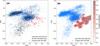 |
Fig. 2 A: same as Fig. 1 but showing A-type and non-A-type asteroids with VIS+NIR spectroscopy after our survey with the IRTF. B: contour plot of the value of the kernel-density estimation ratio Ka(x, y)/Kc(x, y), where x = PC1 and y = PC2, which approximates the probability, P, of finding an A type at (x, y) given there is an asteroid at (x, y), i.e. P(A-type | (x, y)). The kernel densities were calculated here for display with h=0.2. |
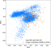 |
Fig. 3 Same as Fig. 1 but showing the PC 1 and PC 2 positions of the A-type candidates selected by DeMeo et al. (2019) from the SDSS that have values within the Gaia DR3. |
5.1 Albedo distribution
We obtained the geometric visible albedos of the A-types in our list from the best-values table of the Minor Planet Physical Properties Catalogue2; these are reported in Tables B.1 and C.2. It is reasonable to assume that the albedo distribution is log-normal, allowing us to calculate an average geometric visible albedo of ![Mathematical equation: $\[0.26_{-0.08}^{+0.11}\]$](/articles/aa/full_html/2026/01/aa56827-25/aa56827-25-eq7.png) , where the asymmetric errors represent the dispersion of the distribution calculated from the symmetric 1 standard deviation of the log pV distribution.
, where the asymmetric errors represent the dispersion of the distribution calculated from the symmetric 1 standard deviation of the log pV distribution.
5.2 Size distribution
To build the size-frequency distribution (SFD) of main-belt A-type asteroids, we must consider that our A-type identification from the Gaia DR3 PC1–PC2 values has meaning only in a statistical sense. Therefore, we adopted a Monte Carlo approach as before; that is, at each iteration, after evaluating P(xi, yi) for each (xi, yi) corresponding to a Gaia DR3 main-belt asteroid, we drew a random number uniformly distributed between 0 and 1. We identified the object as an A-type if the asteroid P value was greater than or equal to the random number. Then, considering only those statistically identified A types with a known diameter, we interpolated their cumulative SFD at each iteration using the interpld function from the scipy.interpolate package in Python. Finally, we calculated the average and standard deviation of these series of interpolated SFDs on a grid of logarithmically spaced diameter values between 1 and 1000 km (Fig. 4). We note that the average of several SFDs is not necessarily a monotonically increasing function with decreasing diameter.
The function calculated as detailed above does not, however, represent the true SFD of main-belt A types, because it must be corrected for the observational biases. To do so, we calculated the ratio between the SFD #6 of Bottke et al. (2020), which is one of the most recent updates of the true main-belt-asteroid SFD and the SFD the of Gaia DR3 main-belt asteroids that have a known diameter. This ratio naturally represents the multiplicative correction that one needs to apply to the Gaia DR3 asteroids with known diameter to obtain the true SFD of the main belt. Hence, we multiplied the Gaia DR3 A-type SFD by the aforementioned ratio for each diameter bin to derive our best estimate of the true SFD of main belt A-type. We present it in Fig. 4, where we can infer between 7000 and 8000 A types with a diameter >2 km. This is a factor ~10 larger than the estimate of DeMeo et al. (2019), and it is similar to our mean A-type abundance in the main belt.
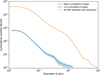 |
Fig. 4 SFD of A-type asteroids from the Gaia DR3 that have a known diameter, uncorrected (blue) and corrected (orange) for observational biases (see text). |
5.3 Heliocentric distribution
We applied the Monte Carlo method, as described in Sect. 3, performing 104 simulations, but selecting asteroids with the orbital proper semi-major axis, ap, within specific intervals corresponding to the major sub-regions of the main belt. Namely, we considered the inner main belt for 2.1 ≤ ap < 2.5 au, the central main belt for 2.5 ≤ ap < 2.82 au, the pristine zone for 2.82 ≤ ap < 2.96 au, and the outer main belt for 2.96 ≤ ap <3.25 au. We took proper orbital elements from the asteroid family portal3 (January 2025 release), where they were computed numerically by means of a synthetic theory by Knežević & Milani (2000); Knežević & Milani (2003). We found mean A-type abundances of (3.25 ± 0.25), (1.91 ± 0.13), (1.51 ± 0.13), and (0.43 ± 0.04)% for these regions, respectively (the number after the ± is the standard deviation of the distribution). This indicates that the abundance of A types in the main belt decreases with increasing heliocentric distance.
When we removed the asteroid members of known collisional families using the family membership definition from Nesvorný et al. (2015), we found that the mean A-type abundances in the aforementioned regions of the main belt are, respectively, (3.0±0.2), (2.10±0.15), (1.8±0.1), and (0.62±0.07)%, still indicating that the abundance of A types in the main belt decreases with increasing heliocentric distance.
5.4 A-type abundance in collisional families
We also applied the Monte Carlo method of Sect. 3 with 104 iterations, selecting asteroids belonging to major collisional families with more than 2000 members. Moreover, as a control for our method, we also included the family (36256) 1999 XT17, which was discovered by Galinier et al. (2024) to have a high abundance of A-type asteroids. We took the family-member definition from Nesvorný et al. (2015). The resulting A-type abundance is shown in Fig. 5, while we found an A-type abundance of (14.1 ± 3.5)% for the (36256) 1999 XT17 family (not shown in plot). The latter is consistent with previous results (Galinier et al. 2024), indicating that our method is robust.
The collisional families investigated here exhibit a significant diversity in A-type asteroid abundance, with values ranging from well below the main-belt average to nearly twice that level. Notably, the family of (36256) 1999 XT17 stands out with an A-type abundance more than seven times higher than the main-belt average. Among the larger families, those of Vesta and Flora show the highest A-type abundances. This is not surprising.
The Vesta family is, among the largest collisional families, the one with the highest A-type asteroid abundance; that is, a value of (4.2 ± 0.5)%. This family consists of fragments ejected by impacts on the asteroid (4) Vesta (Marchi et al. 2012). It is well established that Vesta is a differentiated body (Russell et al. 2012), meaning that its interior separated into a core, mantle, and crust. Ammannito et al. (2013) used DAWN data and suggested that the presence of olivine spots detected on Vesta craters is due to impact excavation processes. However, overall there is no significant olivine on Vesta’s surface. The formation of the two basins of Rheasilvia and Veneneia requires highly energetic impacts, which could have excavated the crust and released olivine-rich fragments that would now be present within the family. The majority of Vesta family members exhibit spectral features similar to those of Vesta’s crustal surface, but a subset may carry signatures indicative of deeper, mantle-derived material. Subsequently, a possibility is that the basins may have been re-covered by basaltic crustal material during their modification stage or by later impacts, hiding traces of the olivine mantle.
Our analysis revealed that the Flora family ranks second among all investigated collisional families in terms of A-type asteroid abundance, with a value of (3.7 ± 0.4)%, which is nearly double the average for the main belt. This finding strongly supports the hypothesis proposed by Oszkiewicz et al. (2015), where a significant population of V- and A-type candidates in the Flora region were identified, potentially indicating the remnants of a differentiated parent body distinct from (4) Vesta. That work, which used taxonomic classification based on SDSS colours, albedos, and phase-curve parameters, suggested that many of these objects cannot be dynamically linked to the Vesta family over the past 100 Myr. Our confirmation of an unusually high fraction of olivine-rich (A-type) material within the Flora family is consistent with this scenario and lends further weight to the idea that Flora may represent the fragments of another differentiated body, although, contrarily to Vesta, only partially.
As a caveat of the above discussion, one would expect these families to exhibit an A-type number density comparable to that of the background asteroids in the inner main belt (the region within which these families are embedded), which is estimated to be (3.0 ± 0.2)%. Since this is not the case, we can infer that the higher than average A-type abundance within the Vesta and Flora families is unlikely to be due to interlopers (see also Fig. 5).
Detecting differentiation in S-complex families originating from parent bodies that are, in general, considered non-differentiated – because they are spectroscopically linked to the ordinary chondrites (Brož et al. 2024b; Marsset et al. 2024 and references therein) – requires some considerations. If the parent body is partially differentiated, this means that the crust could maintain its chondritic composition. Therefore, it should not be surprising to see differentiated and undifferentiated (chondritic) material together. Figure 6 shows the A-type abundance in S-complex collisional families with more than 2000 members as a function of the estimated diameter, Dp, of the family parent body. The latter is calculated as ![Mathematical equation: $\[D_{p}=({\sum}_{i} D_{i}^{3})^{1 / 3}\]$](/articles/aa/full_html/2026/01/aa56827-25/aa56827-25-eq8.png) , where Di is the diameter of the i–th family member (only members with known diameters are included). The values of the Di are taken from the Minor Planet Physical Properties Catalogue, best values, database version 3.3.3-beta. 1 (2025-10-03). The Baptistina family’s symbol is light-toned because its composition is not well constrained: it is indicted as X complex by Nesvorný et al. (2015) and as S complex by Reddy et al. (2009). In addition, the Baptistina family is strongly embedded in the Flora family; the two families show similar A-type abundance. Neglecting Baptistina, Fig. 6 shows a correlation (Pearson correlation ~0.7) between the A-type abundance in S-complex families and the size of their parent bodies, with larger parent bodies exhibiting higher A-type abundances. This could be an indication that larger S-complex parent bodies were more likely to have undergone partial differentiation than smaller ones, which is logical as larger bodies retain more heat than smaller ones (e.g. Trieloff et al. 2022). However, the process of differentiation is complex and depends on various factors, including the body’s size, composition, and the time of the accretion, with the latter strongly controlling the level of internal heating and (partial) differentiation. For example, a body could have started accretion early, within the first 1.5 Myr after the formation of calcium-aluminum inclusions, and then undergone differentiation before continuing its accretion at later times and forming chondritic undifferentiated layers (Weiss & Elkins-Tanton 2013). Moreover, planetesimals can already be implanted into the main belt in a fragmented state from other regions of the Solar System (Avdellidou et al. 2022; Avdellidou et al. 2024). This could also be a possible explanation for the A-type family (36256) 1999 XT17 (Galinier et al. 2024), which is very small. Subsequent family-forming collision in the main belt could have excavated varying amounts of crust and mantle material in order to produce the observed compositional distributions within the families.
, where Di is the diameter of the i–th family member (only members with known diameters are included). The values of the Di are taken from the Minor Planet Physical Properties Catalogue, best values, database version 3.3.3-beta. 1 (2025-10-03). The Baptistina family’s symbol is light-toned because its composition is not well constrained: it is indicted as X complex by Nesvorný et al. (2015) and as S complex by Reddy et al. (2009). In addition, the Baptistina family is strongly embedded in the Flora family; the two families show similar A-type abundance. Neglecting Baptistina, Fig. 6 shows a correlation (Pearson correlation ~0.7) between the A-type abundance in S-complex families and the size of their parent bodies, with larger parent bodies exhibiting higher A-type abundances. This could be an indication that larger S-complex parent bodies were more likely to have undergone partial differentiation than smaller ones, which is logical as larger bodies retain more heat than smaller ones (e.g. Trieloff et al. 2022). However, the process of differentiation is complex and depends on various factors, including the body’s size, composition, and the time of the accretion, with the latter strongly controlling the level of internal heating and (partial) differentiation. For example, a body could have started accretion early, within the first 1.5 Myr after the formation of calcium-aluminum inclusions, and then undergone differentiation before continuing its accretion at later times and forming chondritic undifferentiated layers (Weiss & Elkins-Tanton 2013). Moreover, planetesimals can already be implanted into the main belt in a fragmented state from other regions of the Solar System (Avdellidou et al. 2022; Avdellidou et al. 2024). This could also be a possible explanation for the A-type family (36256) 1999 XT17 (Galinier et al. 2024), which is very small. Subsequent family-forming collision in the main belt could have excavated varying amounts of crust and mantle material in order to produce the observed compositional distributions within the families.
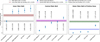 |
Fig. 5 A-type abundance (with values) in collisional families with more than 2000 members according to the definition of Nesvorný et al. (2015), compared to the average value of the main belt and the host region of the family in the belt (inner, central, outer). Values per family, given within the plot, are percentages. The values after the ± symbol represent the standard deviation of the distribution of the A-type abundance. |
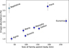 |
Fig. 6 A-type abundance in S-complex collisional families with more than 2000 members according to the definition of Nesvorný et al. (2015) as a function of the estimated diameter of the family parent body. |
6 Conclusions
We performed a statistical and spectroscopic analysis of A-type asteroids in the main belt by combining Gaia DR3 VIS reflectance spectra with ground-based NIR observations. Our classification pipeline identified a population of A-type candidates, and we confirmed several of them with IRTF observations. We combined our observations with literature data, allowing us to derive a new estimate of the A-type abundance across the main belt, which we found to be (2.00 ± 0.15)%, a significantly higher fraction than previous studies had suggested.
By examining the abundance of A types within known collisional families, we discovered a marked diversity: some families, such as Vesta and Flora, exhibit above-average A-type fractions, whereas others, such as Themis and Hygiea, display an almost complete absence of this asteroid type. The Flora family, in particular, stands out as the second most A-type-rich large family, in line with the results of Oszkiewicz et al. (2015), who hypothesised the existence of a second differentiated parent body in the inner main belt in addition to (4) Vesta.
These findings lend new observational support to the idea that olivine-rich materials – and, by extension, fragments of differentiated bodies – are more common in the asteroid belt than previously thought. This suggests that either differentiation was more widespread in the early solar system or that our past observational constraints were incomplete. Our work thus contributes to resolving the long-standing missing-mantle problem and opens new avenues for identifying remnants of early planetary building blocks.
This work highlights the scientific potential of combining visible-light data from Gaia DR3 with NIR spectrophotometry for the taxonomic classification of asteroids. In particular, it demonstrates the value of broad-wavelength coverage for identifying and confirming rare asteroid types such as A types. Looking forward, NASA’s SPHEREx mission is expected to deliver NIR spectrophotometry for a vast number of Solar System objects (Lisse et al. 2024). When combined with Gaia DR3 reflectance spectra, SPHEREx will enable the compilation of a powerful, multi-band spectral dataset that will allow for the systematic and robust taxonomic classification of, hopefully, most of the asteroids present in Gaia DR3. Our results anticipate the potential of such a dataset both to improve the estimation of Eq. (A.1) across different taxonomic classes and to enable the direct identification of rare classes, thereby providing a preview of the transformative science it will make possible.
Acknowledgements
We acknowledge support from the ANR ORIGINS (ANR-18-CE31-0014) and the French Space Agency CNES. U.B. acknowledges funding from an STFC PhD studentship. This work has made use of data from the European Space Agency (ESA) mission Gaia (https://www.cosmos.esa.int/gaia), processed by the Gaia Data Processing and Analysis Consortium (DPAC, https://www.cosmos.esa.int/web/gaia/dpac/consortium). Funding for the DPAC has been provided by national institutions, in particular the institutions participating in the Gaia Multilateral Agreement. This work is based on data provided by the Minor Planet Physical Properties Catalogue (MP3C) of the Observatoire de la Côte d’Azur. C.A. and M.D. were Visiting Astronomers at the Infrared Telescope Facility, which is operated by the University of Hawaii under contract 80HQTR19D0030 with the National Aeronautics and Space Administration.
References
- Ammannito, E., de Sanctis, M. C., Palomba, E., et al. 2013, Nature, 504, 122 [Google Scholar]
- Avdellidou, C., Delbo, M., Morbidelli, A., et al. 2022, A&A, 665, L9 [NASA ADS] [CrossRef] [EDP Sciences] [Google Scholar]
- Avdellidou, C., Delbo’, M., Nesvorný, D., Walsh, K. J., & Morbidelli, A. 2024, Science, 384, 348 [CrossRef] [Google Scholar]
- Avdellidou, C., Bhat, U., Bujdoso, K., et al. 2025, MNRAS, 539, 3534 [Google Scholar]
- Bell, J. F., Davis, D. R., Hartmann, W. K., & Gaffey, M. J. 1989, in Asteroids II, eds. R. P. Binzel, T. Gehrels, & M. S. Matthews (Tucson: University of Arizona Press), 921 [Google Scholar]
- Benedix, G., Haack, H., & McCoy, T. 2014, in Treatise on Geochemistry (Amsterdam: Elsevier), 267 [Google Scholar]
- Binzel, R. P., Birlan, M., Bus, S. J., et al. 2004, P&SS, 52, 291 [Google Scholar]
- Binzel, R. P., DeMeo, F. E., Turtelboom, E. V., et al. 2019, Icarus, 324, 41 [Google Scholar]
- Bottke, W. F., Vokrouhlický, D., Ballouz, R. L., et al. 2020, AJ, 160, 14 [Google Scholar]
- Bourdelle de Micas, J., Fornasier, S., Avdellidou, C., et al. 2022, A&A, 665, A83 [NASA ADS] [CrossRef] [EDP Sciences] [Google Scholar]
- Brož, M., Morbidelli, A., Bottke, W. F., et al. 2013, A&A, 551, A117 [Google Scholar]
- Brož, M., Vernazza, P., Marsset, M., et al. 2024a, A&A, 689, A183 [NASA ADS] [CrossRef] [EDP Sciences] [Google Scholar]
- Brož, M., Vernazza, P., Marsset, M., et al. 2024b, Nature, 634, 566 [Google Scholar]
- Burbine, T. H., & Binzel, R. P. 2002, Icarus, 159, 468 [CrossRef] [Google Scholar]
- Burbine, T., McCoy, T. J., Meibom, A., Gladman, B., & Keil, K. 2002, in Asteroids III (Tucson: University of Ariziona Press) [Google Scholar]
- Bus, S., & Binzel, R. 2002, Icarus, 158, 146 [NASA ADS] [CrossRef] [Google Scholar]
- Chapman, C. R. 1986, Mem. Soc. Astron. Italiana, 57, 103 [Google Scholar]
- Choi, S., Moon, H.-K., Roh, D.-G., et al. 2023, PSJ, 4, 49 [Google Scholar]
- Cushing, M. C., Vacca, W. D., & Rayner, J. T. 2004, PNAS, 116, 362 [Google Scholar]
- de León, J., Licandro, J., Serra-Ricart, M., Pinilla-Alonso, N., & Campins, H. 2010, A&A, 517, A23 [CrossRef] [EDP Sciences] [Google Scholar]
- Delbo’, M., Walsh, K., Bolin, B., Avdellidou, C., & Morbidelli, A. 2017, Science, 357, 1026 [NASA ADS] [CrossRef] [Google Scholar]
- Delbo, M., Avdellidou, C., & Morbidelli, A. 2019, A&A, 624, A69 [NASA ADS] [CrossRef] [EDP Sciences] [Google Scholar]
- Delbo, M., Avdellidou, C., & Walsh, K. J. 2023, A&A, 680, A105 [NASA ADS] [CrossRef] [EDP Sciences] [Google Scholar]
- DeMeo, F., & Carry, B. 2013, Icarus, 226, 723 [NASA ADS] [CrossRef] [Google Scholar]
- DeMeo, F. E., Binzel, R. P., Slivan, S. M., & Bus, S. J. 2009, Icarus, 202, 160 [Google Scholar]
- DeMeo, F. E., Polishook, D., Carry, B., et al. 2019, Icarus, 322, 13 [CrossRef] [Google Scholar]
- Dermott, S. F., Christou, A. A., Li, D., Kehoe, Thomas. J. J., & Robinson, J. M. 2018, Nat. Astron., 2, 549 [NASA ADS] [CrossRef] [Google Scholar]
- Devogèle, M., Moskovitz, N., Thirouin, A., et al. 2019, AJ, 158, 196 [CrossRef] [Google Scholar]
- Ferrone, S., Delbo, M., Avdellidou, C., et al. 2023, A&A, 676, A5 [NASA ADS] [CrossRef] [EDP Sciences] [Google Scholar]
- Fornasier, S., Migliorini, A., Dotto, E., & Barucci, M. A. 2008, Icarus, 196, 119 [NASA ADS] [CrossRef] [Google Scholar]
- Fornasier, S., Clark, B. E., & Dotto, E. 2011, Icarus, 214, 131 [NASA ADS] [CrossRef] [Google Scholar]
- Gaia Collaboration (Galluccio, L., et al.) 2023, A&A, 674, A35 [NASA ADS] [CrossRef] [EDP Sciences] [Google Scholar]
- Galinier, M., Delbo, M., Avdellidou, C., & Galluccio, L. 2024, A&A, 683, L3 [NASA ADS] [CrossRef] [EDP Sciences] [Google Scholar]
- Galinier, M., Delbo, M., Avdellidou, C., Galluccio, L., & Marrocchi, Y. 2023, A&A, 671, A40 [NASA ADS] [CrossRef] [EDP Sciences] [Google Scholar]
- Gietzen, K. M., Lacy, C. H. S., Ostrowski, D. R., & Sears, D. W. G. 2012, MAPS, 47, 1789 [NASA ADS] [Google Scholar]
- Greenwood, R. C., Burbine, T. H., & Franchi, I. A. 2020, Geochim. Cosmochim. Acta., 277, 377 [NASA ADS] [CrossRef] [Google Scholar]
- Gulbis, A. A. S., Bus, S. J., Elliot, J. L., et al. 2011, PNAS, 123, 461 [Google Scholar]
- Harris, A. W., & Drube, L. 2014, ApJ, 785, L4 [NASA ADS] [CrossRef] [Google Scholar]
- Hasegawa, S., Marsset, M., DeMeo, F. E., et al. 2024, AJ, 167, 224 [CrossRef] [Google Scholar]
- Klahr, H., Delbo, M., & Gerbig, K. 2022, in Vesta and Ceres: Insights from the Dawn Mission for the Origin of the Solar System (Cambridge: Cambridge University Press), 199 [Google Scholar]
- Knežević, Z., & Milani, A. 2000, CMDA, 78, 17 [Google Scholar]
- Knežević, Z., & Milani, A. 2003, A&A, 403, 1165 [Google Scholar]
- Lauretta, D. S., Connolly, H. C., Aebersold, J. E., et al. 2024, MAPS, 59, 2453 [Google Scholar]
- Lazzarin, M., Marchi, S., Magrin, S., & Licandro, J. 2005, MNRAS, 359, 1575 [Google Scholar]
- Leith, T. B., Moskovitz, N. A., Mayne, R. G., et al. 2017, Icarus, 295, 61 [NASA ADS] [CrossRef] [Google Scholar]
- Lisse, C. M., Bauer, J., Kim, Y., et al. 2024, in AGU Fall Meeting Abstracts, 2024, P43F-02 [Google Scholar]
- Lucas, M. P., Emery, J. P., MacLennan, E. M., et al. 2019, Icarus, 322, 227 [NASA ADS] [CrossRef] [Google Scholar]
- MacPherson, G. J., Davis, A. M., & Zinner, E. K. 1995, Meteoritics, 30, 365 [Google Scholar]
- Mahlke, M., Carry, B., & Mattei, P.-A. 2022, A&A, 665, A26 [NASA ADS] [CrossRef] [EDP Sciences] [Google Scholar]
- Marchi, S., McSween, H. Y., O’Brien, D. P., et al. 2012, Science, 336, 690 [NASA ADS] [CrossRef] [Google Scholar]
- Marsset, M., DeMeo, F. E., Burt, B., et al. 2022, AJ, 163, 165 [NASA ADS] [CrossRef] [Google Scholar]
- Marsset, M., Vernazza, P., Brož, M., et al. 2024, Nature, 634, 561 [Google Scholar]
- Morbidelli, A., Kleine, T., & Nimmo, F. 2025, EPSL, 650, 119120 [Google Scholar]
- Moskovitz, N. A., Lawrence, S., Jedicke, R., et al. 2008, ApJ, 682, L57 [NASA ADS] [CrossRef] [Google Scholar]
- Nesvorný, D., Broz, M., & Carruba, V. 2015, in Asteroids IV, eds. P. Michel, F. E. DeMeo, & W. F. Bottke (Tucson: University of Arizona Press) [Google Scholar]
- Nesvorný, D., Roig, F., Vokrouhlický, D., & Brož, M. 2024, ApJS, 274, 25 [Google Scholar]
- Neumann, W., Breuer, D., & Spohn, T. 2012, A&A, 543, A141 [NASA ADS] [CrossRef] [EDP Sciences] [Google Scholar]
- Oszkiewicz, D., Kankiewicz, P., Włodarczyk, I., & Kryszczyńska, A. 2015, A&A, 584, A18 [NASA ADS] [CrossRef] [EDP Sciences] [Google Scholar]
- Pedregosa, F., Pedregosa, F., Varoquaux, G., et al. 2011, JMLR, 12, 2825 [Google Scholar]
- Perna, D., Barucci, M. A., Fulchignoni, M., et al. 2018, P&SS, 157, 82 [Google Scholar]
- Popescu, M., Licandro, J., Carvano, J. M., et al. 2018, A&A, 617, A12 [NASA ADS] [CrossRef] [EDP Sciences] [Google Scholar]
- Rayner, J. T., Toomey, D. W., Onaka, P. M., et al. 2003, PNAS, 115, 362 [Google Scholar]
- Reddy, V., Emery, J. P., Gaffey, M. J., et al. 2009, MAPS, 44, 1917 [NASA ADS] [Google Scholar]
- Russell, C. T., Raymond, C. A., Coradini, A., et al. 2012, Science, 336, 684 [NASA ADS] [CrossRef] [Google Scholar]
- Sanchez, J. A., Reddy, V., Kelley, M. S., et al. 2014, Icarus, 228, 288 [CrossRef] [Google Scholar]
- Sergeyev, A. V., Carry, B., Marsset, M., et al. 2023, A&A, 679, A148 [NASA ADS] [CrossRef] [EDP Sciences] [Google Scholar]
- Solontoi, M. R., Hammergren, M., Gyuk, G., & Puckett, A. 2012, Icarus, 220, 577 [NASA ADS] [CrossRef] [Google Scholar]
- Spoto, F., Milani, A., & Knežević, Z. 2015, Icarus, 257, 275 [NASA ADS] [CrossRef] [Google Scholar]
- Tanga, P., Pauwels, T., Mignard, F., et al. 2023, A&A, 674, A12 [NASA ADS] [CrossRef] [EDP Sciences] [Google Scholar]
- Tinaut-Ruano, F., Tatsumi, E., Tanga, P., et al. 2023, A&A, 669, L14 [NASA ADS] [CrossRef] [EDP Sciences] [Google Scholar]
- Trieloff, M., Hopp, J., & Gail, H.-P. 2022, Icarus, 373, 114762 [NASA ADS] [CrossRef] [Google Scholar]
- Urey, H. C. 1955, Proc. Natl. Acad. Sci., 41, 127 [Google Scholar]
- Weiss, B. P., & Elkins-Tanton, L. T. 2013, Annu. Rev. Earth Planet. Sci.s, 41, 529 [Google Scholar]
https://mp3c.oca.eu (version 3.2.1-beta. 1 of 2024-08-12).
Appendix A A-type probability estimation
Having the two sets of asteroids, namely, A-type and non A-type from VIS+NIR spectroscopy from the literature and our own survey, we defined the two sets of asteroids, i.e. the ![Mathematical equation: $\[\mathcal{S}_{A}=\left\{\left(x_{i}, y_{i}\right)\right\}_{i=1}^{N}\]$](/articles/aa/full_html/2026/01/aa56827-25/aa56827-25-eq9.png) and the
and the ![Mathematical equation: $\[\mathcal{S}_{\tilde{A}}=\left\{\left(x_{j}, y_{j}\right)\right\}_{j=1}^{\tilde{N}}\]$](/articles/aa/full_html/2026/01/aa56827-25/aa56827-25-eq10.png) , where i and j are indexes running on the set of the N asteroids classified as A-type and on the
, where i and j are indexes running on the set of the N asteroids classified as A-type and on the ![Mathematical equation: $\[\tilde{N}\]$](/articles/aa/full_html/2026/01/aa56827-25/aa56827-25-eq11.png) non A-types ones. We then defined the 𝒞 set to be the union of the previously two defined sets, namely,
non A-types ones. We then defined the 𝒞 set to be the union of the previously two defined sets, namely, ![Mathematical equation: $\[\mathcal{C}=\mathcal{S}_{A} \cup \mathcal{S}_{\tilde{A}}\]$](/articles/aa/full_html/2026/01/aa56827-25/aa56827-25-eq12.png) . Since the sets 𝒮A and
. Since the sets 𝒮A and ![Mathematical equation: $\[\mathcal{S}_{\tilde{A}}\]$](/articles/aa/full_html/2026/01/aa56827-25/aa56827-25-eq13.png) are disjoint, i.e.
are disjoint, i.e. ![Mathematical equation: $\[\mathcal{S}_{A} \cap \mathcal{S}_{\tilde{A}}=\emptyset\]$](/articles/aa/full_html/2026/01/aa56827-25/aa56827-25-eq14.png) , then the total number of elements in the union is
, then the total number of elements in the union is ![Mathematical equation: $\[|\mathcal{C}|=\left|\mathcal{S}_{A} \cup \mathcal{S}_{\tilde{A}}\right|=N+\tilde{N}\]$](/articles/aa/full_html/2026/01/aa56827-25/aa56827-25-eq15.png) .
.
We also defined the distributions ![Mathematical equation: $\[a(x, y)={\sum}_{i}^{N} \delta(x-x_{i}, y-y_{i})\]$](/articles/aa/full_html/2026/01/aa56827-25/aa56827-25-eq16.png) and
and ![Mathematical equation: $\[\tilde{a}(x, y)={\sum}_{j}^{\tilde{N}} \delta\left(x-x_{j}, y-y_{j}\right)\]$](/articles/aa/full_html/2026/01/aa56827-25/aa56827-25-eq17.png) , where i and j are indexes running on the set 𝒮A and the set
, where i and j are indexes running on the set 𝒮A and the set ![Mathematical equation: $\[\mathcal{S}_{\tilde{A}}\]$](/articles/aa/full_html/2026/01/aa56827-25/aa56827-25-eq18.png) , respectively, while δ(x − x0, y − y0) is the Dirac delta function that is non-zero only at x = x0, y = y0 and has the property that ∫∫ δ(x − x0, y − y0)dxdy = 1. Having noted that ∫∫ a(x, y)dxdy = N and
, respectively, while δ(x − x0, y − y0) is the Dirac delta function that is non-zero only at x = x0, y = y0 and has the property that ∫∫ δ(x − x0, y − y0)dxdy = 1. Having noted that ∫∫ a(x, y)dxdy = N and ![Mathematical equation: $\[\iint \tilde{a}(x, y) d x d y=\tilde{N}\]$](/articles/aa/full_html/2026/01/aa56827-25/aa56827-25-eq19.png) , one could be tempted to assume that the probability P to have an A-type at (x, y) (given that there is an asteroid at (x, y)), i.e.
, one could be tempted to assume that the probability P to have an A-type at (x, y) (given that there is an asteroid at (x, y)), i.e.
![Mathematical equation: $\[P(\text {A-type } \mid(x, y))=\frac{\text { number density of A-type asteroids at }(x. y)}{\text { number density of classified asteroids at }(x, y)}\]$](/articles/aa/full_html/2026/01/aa56827-25/aa56827-25-eq20.png) (A.1)
(A.1)
can be given by a(x, y)/c(x, y) where ![Mathematical equation: $\[c(x, y)=a(x, y)+\tilde{a}(x, y)\]$](/articles/aa/full_html/2026/01/aa56827-25/aa56827-25-eq21.png) represents all the asteroids that have an A-type class together with those that have a class that is not A-type, both classified from VIS+NIR spectroscopy. Since both a(x, y) and c(x, y) are sums of Dirac delta functions, this ratio is not a smooth function, but is rather defined only at locations where c(x, y) ≠ 0. Namely, if (x, y) corresponds to an A-type, then a(x, y) = δ and c(x, y) = δ, hence a(x, y)/c(x, y) = 1, whereas when (x, y) corresponds to a non A-type, then a(x, y) = 0 and c(x, y) = δ, hence, a(x, y)/c(x, y) = 0. But if (x, y) does not correspond to any objects represented by the c(x, y) function the ratio a(x, y)/c(x, y) is undefined. The latter situation is, precisely, our case, because we aim at evaluating P(A-type | (x, y)) at those points where Gaia DR3 asteroids exist, which is a more numerous set of objects than those represented by the c(x, y) function.
represents all the asteroids that have an A-type class together with those that have a class that is not A-type, both classified from VIS+NIR spectroscopy. Since both a(x, y) and c(x, y) are sums of Dirac delta functions, this ratio is not a smooth function, but is rather defined only at locations where c(x, y) ≠ 0. Namely, if (x, y) corresponds to an A-type, then a(x, y) = δ and c(x, y) = δ, hence a(x, y)/c(x, y) = 1, whereas when (x, y) corresponds to a non A-type, then a(x, y) = 0 and c(x, y) = δ, hence, a(x, y)/c(x, y) = 0. But if (x, y) does not correspond to any objects represented by the c(x, y) function the ratio a(x, y)/c(x, y) is undefined. The latter situation is, precisely, our case, because we aim at evaluating P(A-type | (x, y)) at those points where Gaia DR3 asteroids exist, which is a more numerous set of objects than those represented by the c(x, y) function.
A common solution to this problem is to smooth the sum of Dirac delta distributions by a kernel function of the form k(x − xi, y − yi) = exp[−((x − xi)2 + (y − yi)2)/(2h2)], where h is the so-called smoothing factor (also known as bandwidth). To implement this method, we defined
![Mathematical equation: $\[K_a(x, y)=\frac{1}{\left(h^2 2 \pi\right)} \sum_{i=1}^N k\left(x-x_i, y-y_i\right) \text { and }\]$](/articles/aa/full_html/2026/01/aa56827-25/aa56827-25-eq22.png) (A.2)
(A.2)
![Mathematical equation: $\[K_c(x, y)=K_a(x, y)+\frac{1}{\left(h^2 2 \pi\right)} \sum_{j=1}^{\tilde{N}} k\left(x-x_j, y-y_j\right)\]$](/articles/aa/full_html/2026/01/aa56827-25/aa56827-25-eq23.png) (A.3)
(A.3)
to represent the kernel density estimations of the PC1–PC2 values of the set 𝒮A of the A-types, and the 𝒮𝒞 set of non A-types together with the A-types (from VIS+NIR spectroscopy), respectively. By construction, ∫∫ Ka(x, y)dxdy = N and ![Mathematical equation: $\[\iint K_{c}(x, y) d x d y=N+\tilde{N}\]$](/articles/aa/full_html/2026/01/aa56827-25/aa56827-25-eq24.png) , hence, Ka(x, y)/Kc(x, y) ~ P(A-type | (x, y)) approximates the local probability of finding an A-type asteroid at location (x, y). The abundance of A-types within the Gaia DR3 can thus be estimated by calculating the quantity
, hence, Ka(x, y)/Kc(x, y) ~ P(A-type | (x, y)) approximates the local probability of finding an A-type asteroid at location (x, y). The abundance of A-types within the Gaia DR3 can thus be estimated by calculating the quantity
![Mathematical equation: $\[N_{\mathrm{A}} / N_{\mathrm{MB}}=1 / N_{\mathrm{MB}} \sum_{k=1}^{N_{\mathrm{MB}}} K_a(x_k, y_k) / K_c(x_k, y_k),\]$](/articles/aa/full_html/2026/01/aa56827-25/aa56827-25-eq25.png) (A.4)
(A.4)
where the index k runs over the set of NMB asteroids within the main belt that have PC1, PC2 values equal to (xk, yk), respectively.
We used the KernelDensity Python class from the scikit-learn project (Pedregosa et al. 2011) for the estimation of the Ka(x, y) and Kc(x, y) functions. Instead of attempting to find the most suitable values for the smoothing factor, we used its properties to estimate the uncertainty on the value of Ka(x, y)/Kc(x, y). Namely, we performed a Monte Carlo simulation where at each iteration a random value of the smoothing factor was extracted from a uniform distribution between 10−1 and 100, with these limits corresponding to cases that where determined visually to overfit and under-fit the data, respectively. At each iteration, we calculated Ka(x, y) by summing on ![Mathematical equation: $\[N-\sqrt{N}\left(x_{i}, y_{i}\right)\]$](/articles/aa/full_html/2026/01/aa56827-25/aa56827-25-eq26.png) points randomly extracted without repetition from the set 𝒮A and the function Kc(x, y) by summing on
points randomly extracted without repetition from the set 𝒮A and the function Kc(x, y) by summing on ![Mathematical equation: $\[N+\tilde{N}-\sqrt{N+\tilde{N}}\left(x_{j}, y_{j}\right)\]$](/articles/aa/full_html/2026/01/aa56827-25/aa56827-25-eq27.png) points also randomly extracted without repetition from the set 𝒞. So, at each iteration we evaluated the ratio Ka(x, y)/Kc(x, y) to approximate P(A-type | (x, y)) and then NA/NMB from Eq.A.4.
points also randomly extracted without repetition from the set 𝒞. So, at each iteration we evaluated the ratio Ka(x, y)/Kc(x, y) to approximate P(A-type | (x, y)) and then NA/NMB from Eq.A.4.
Appendix B Literature A-type asteroids
Forty-four main belt and Mars-crosser asteroids classified as A-types in the literature using their VIS and NIR part of the spectrum that are also incl
Appendix C Observations of candidate A-types and results
Observational circumstances for NIR spectroscopy of the 88 asteroids of our programme.
Physical properties and our spectral classification of the 88 asteroids observed in this work.
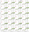 |
Fig. C.1 Reflectance spectra of the asteroids from this work. Reflectance spectra from the SpeX instrument at the IRTF, Gaia DR3 and (when available SDSS are shown with grey stars, black filled circles and red filled circles, respectively. The green shaded areas represent the range of spectra for the A-types of the Bus-DeMeo taxonomy (DeMeo et al. 2009) for comparison to the observed reflectance spectra. The grey-shaded regions correspond to wavelength range of lower atmospheric transparency. Data in those regions, should be interpreted with care. Asteroids numbers from 254 to 3104 are shown here. |
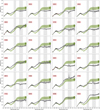 |
Fig. C.2 Reflectance spectra of the asteroids from this work. Asteroids numbers from 3272 to 8660 are shown here. See the caption of Fig. C.1 for further details. |
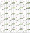 |
Fig. C.3 Reflectance spectra of the asteroids from this work. Asteroids numbers from 10017 to 22849 are shown here. See the caption of Fig. C.1 for further details. |
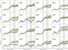 |
Fig. C.4 Reflectance spectra of the asteroids from this work. Asteroids numbers from 24473 to 141111 are shown here. See the caption of Fig. C.1 for further details. |
Appendix D Distribution of the main spectral types
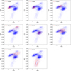 |
Fig. D.1 Distribution of several Bus-DeMeo taxonomic classes, as indicated in the plot legend, on the PC1–PC2 plane for asteroids with Gaia DR3 reflectance spectra and S/N > 30 (shown as grey points). |
All Tables
Forty-four main belt and Mars-crosser asteroids classified as A-types in the literature using their VIS and NIR part of the spectrum that are also incl
Observational circumstances for NIR spectroscopy of the 88 asteroids of our programme.
Physical properties and our spectral classification of the 88 asteroids observed in this work.
All Figures
|
Fig. 1 PC1 versus PC2 plot of main-belt asteroid reflectance spectra from the Gaia DR3 with S/N>50 (blue circles; see Gaia Collaboration 2023 for details of the S/N estimation). The red stars indicate the A types that we selected from the literature following the method explained in the text and that also have a DR3 reflectance spectrum. The green triangles show the asteroids that we observed with the IRTF. |
| In the text | |
|
Fig. 2 A: same as Fig. 1 but showing A-type and non-A-type asteroids with VIS+NIR spectroscopy after our survey with the IRTF. B: contour plot of the value of the kernel-density estimation ratio Ka(x, y)/Kc(x, y), where x = PC1 and y = PC2, which approximates the probability, P, of finding an A type at (x, y) given there is an asteroid at (x, y), i.e. P(A-type | (x, y)). The kernel densities were calculated here for display with h=0.2. |
| In the text | |
|
Fig. 3 Same as Fig. 1 but showing the PC 1 and PC 2 positions of the A-type candidates selected by DeMeo et al. (2019) from the SDSS that have values within the Gaia DR3. |
| In the text | |
|
Fig. 4 SFD of A-type asteroids from the Gaia DR3 that have a known diameter, uncorrected (blue) and corrected (orange) for observational biases (see text). |
| In the text | |
|
Fig. 5 A-type abundance (with values) in collisional families with more than 2000 members according to the definition of Nesvorný et al. (2015), compared to the average value of the main belt and the host region of the family in the belt (inner, central, outer). Values per family, given within the plot, are percentages. The values after the ± symbol represent the standard deviation of the distribution of the A-type abundance. |
| In the text | |
|
Fig. 6 A-type abundance in S-complex collisional families with more than 2000 members according to the definition of Nesvorný et al. (2015) as a function of the estimated diameter of the family parent body. |
| In the text | |
|
Fig. C.1 Reflectance spectra of the asteroids from this work. Reflectance spectra from the SpeX instrument at the IRTF, Gaia DR3 and (when available SDSS are shown with grey stars, black filled circles and red filled circles, respectively. The green shaded areas represent the range of spectra for the A-types of the Bus-DeMeo taxonomy (DeMeo et al. 2009) for comparison to the observed reflectance spectra. The grey-shaded regions correspond to wavelength range of lower atmospheric transparency. Data in those regions, should be interpreted with care. Asteroids numbers from 254 to 3104 are shown here. |
| In the text | |
|
Fig. C.2 Reflectance spectra of the asteroids from this work. Asteroids numbers from 3272 to 8660 are shown here. See the caption of Fig. C.1 for further details. |
| In the text | |
|
Fig. C.3 Reflectance spectra of the asteroids from this work. Asteroids numbers from 10017 to 22849 are shown here. See the caption of Fig. C.1 for further details. |
| In the text | |
|
Fig. C.4 Reflectance spectra of the asteroids from this work. Asteroids numbers from 24473 to 141111 are shown here. See the caption of Fig. C.1 for further details. |
| In the text | |
|
Fig. D.1 Distribution of several Bus-DeMeo taxonomic classes, as indicated in the plot legend, on the PC1–PC2 plane for asteroids with Gaia DR3 reflectance spectra and S/N > 30 (shown as grey points). |
| In the text | |
Current usage metrics show cumulative count of Article Views (full-text article views including HTML views, PDF and ePub downloads, according to the available data) and Abstracts Views on Vision4Press platform.
Data correspond to usage on the plateform after 2015. The current usage metrics is available 48-96 hours after online publication and is updated daily on week days.
Initial download of the metrics may take a while.