| Issue |
A&A
Volume 705, January 2026
|
|
|---|---|---|
| Article Number | A224 | |
| Number of page(s) | 11 | |
| Section | Atomic, molecular, and nuclear data | |
| DOI | https://doi.org/10.1051/0004-6361/202557146 | |
| Published online | 23 January 2026 | |
New experimental and theoretical energy levels, lifetimes, and oscillator strengths in singly ionised zirconium
1
Division of Astrophysics, Department of Physics, Lund University,
Box 43,
221 00
Lund,
Sweden
2
Material Science and Applied Mathematics, Malmö University,
205 06
Malmö,
Sweden
3
Division of Atomic Physics, Department of Physics, Lund University,
Box 118,
221 00,
Lund,
Sweden
4
Physique Atomique et Astrophysique, Université de Mons,
7000
Mons,
Belgium
5
IPNAS, Université de Liège,
4000
Liège,
Belgium
★ Corresponding authors: This email address is being protected from spambots. You need JavaScript enabled to view it.
; This email address is being protected from spambots. You need JavaScript enabled to view it.
Received:
8
September
2025
Accepted:
9
November
2025
Abstract
Context. Neutron-capture elements are believed to make up almost all elements heavier than iron in the periodic table. By studying the abundance of these elements throughout the Galaxy, it is possible to put constraints on how and where neutron-capture processes occur. Determining elemental abundances is made possible through the correct interpretation and modelling of astrophysical spectra. Key ingredients for this, in turn, are accurate and complete sets of atomic data.
Aims. We investigate the spectrum of singly ionised zirconium with the aim of reporting level energies and radiative lifetimes for previously experimentally unknown high-lying even 4d26s and 4d25d levels, as well as improved energies for odd 4d25p and 4d5s5p levels. We also aim to provide wavelengths, branching fractions, and oscillator strengths (log gf values) for lines from these upper even 4d26s and 4d25d levels.
Methods. The energies, wavelengths, and branching fractions were derived from hollow cathode spectra recorded with a Fourier transform spectrometer. The radiative lifetimes were measured using a two-step laser-induced fluorescence technique. Theoretical calculations using the pseudo-relativistic Hartree-Fock method, modified to account for core polarisation effects, were also performed and show good general agreement with the experimental results.
Results. We report for the first time level energies and radiative lifetimes for 19 high-lying even 4d26s and 4d25d levels and improved energies for odd 15 4d25p and 4d5s5p levels in Zr II. We also report wavelengths, branching fractions, and oscillator strengths for 79 lines from upper levels of 4d26s and 4d25d.
Key words: atomic data / methods: laboratory: atomic / techniques: spectroscopic
© The Authors 2026
 Open Access article, published by EDP Sciences, under the terms of the Creative Commons Attribution License (https://creativecommons.org/licenses/by/4.0), which permits unrestricted use, distribution, and reproduction in any medium, provided the original work is properly cited.
This article is published in open access under the Subscribe to Open model. This email address is being protected from spambots. You need JavaScript enabled to view it. to support open access publication.
1 Introduction
Zirconium is predominantly produced by the slow neutron capture process (s-process) in massive stars and is therefore labelled an ‘s-process’ element, although non-negligible contributions from the rapid neutron capture process (r-process) also play a role. However, there is still some ambiguity regarding the origin of the total amount of observed zirconium. Different Galactic chemical evolution models suggest various production sites, either as an additional neutron capture process (see e.g. Travaglio et al. 2004), or as the result of the not yet fully understood processes within the stellar convective envelope (e.g. Molero et al. 2023; Forsberg et al. 2019). Further investigation of zirconium and other s-process elements is therefore needed to bring clarity to this.
An additional motivation for the present work is that it may serve as a benchmark for theoretical atomic structure calculations. An open d-shell and three close-lying low even configurations give zirconium a complex structure with multiple series limits (see Figure 1), making it challenging to compute. This is especially true for states of higher excitation, such as those targeted in this paper, for which more electron correlation is needed to accurately describe the atomic structure (Froese-Fischer et al. 1997).
The spectrum of singly ionised zirconium was studied in 1930 by Kiess & Kiess (1930), who identified 735 Zr II lines in the wavelength range from 1740 to 6790 Â. They reported 125 levels belonging to the 4d25s, 4d3 , 4d5s2, 4d26s, 4d25d, 4d25p, and 4d5s5p configurations. More recently, Lawler et al. (2022) reported updated energies for 36 Zr II levels and 87 Zr I levels. For Zr II, this includes the even-parity levels of the 4d25s and 4d3 configurations, as well as the odd-parity levels of the 4d25p configuration.
Biemont et al. (1981) reported oscillator strengths for 24 transitions in Zr II, derived by combining lifetimes and branching fractions (BFs). They also reported 34 oscillator strengths for Zr I lines and the solar abundance of zirconium. Sikström et al. (1999) reported lifetimes of six levels, out of which three have lifetimes on the sub-nanosecond scale. In addition, they reported BFs for three levels and derived oscillator strengths for 27 Zr II lines. Langhans et al. (1995) reported 18 lifetimes in Zr II. Ljung et al. (2006) reported 263 BFs in Zr II and derived oscillator strengths by combining the BFs with lifetimes from Biemont et al. (1981), Sikström et al. (1999), and Langhans et al. (1995). Malcheva et al. (2006) published lifetimes for 12 levels in Zr II and HFR calculations benchmarked with experimental lifetimes.
All measurements in Zr II so far have dealt with lifetimes and BFs from the odd 4d25p and 4d5s5p configurations. However, in this paper we study the high even configurations 4d26s and 4d25d. We report 19 previously unknown even-parity energy levels, together with the corresponding experimental lifetimes, and improved energies for 15 4d25p and 4d5s5p oddparity levels in Zr II. We also report wavelengths, together with BFs and oscillator strengths (log gf-values) for 79 lines.
In Section 2 we present the details of the experimental part of the project, starting with the Fourier transform spectrometer (FTS) spectra and intensity measurements, from which the energy levels and BF s are derived, followed by the lifetime measurements, which combined with the BFs lead to the log gf -values. Section 3 describes the theoretical calculations, and in Section 4 we present and discuss our results.
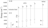 |
Fig. 1 Partial energy level diagram of Zr II. |
2 Experiment
The experiments are divided into two parts. First, we discuss the spectral analysis leading to wavelengths, BFs, and energy levels. Then, in Section 2.5, we describe measurements of radiative lifetimes of the high-lying even-parity levels.
2.1 FTS spectra
The wavelengths and BFs were measured from intensity-calibrated spectra recorded with an FTS (Chelsea Instrument FT500 UV FTS). The spectra were recorded between 20 500 and 41 000 cm−1. A hollow cathode discharge lamp (HCL), producing the zirconium ions, was used as the light source. The HCL was run with currents between 0.15 and 0.5 A, using 0.6 Torr argon as the carrier gas. The signal was recorded in the second alias and with a resolution of 0.055 cm−1, using a Hamamatsu 1P28 photo multiplier tube. The interferograms were phase-corrected and Fourier-transformed using the computer code Xgremlin (Nave et al. 1997). An example spectrum is shown in Figure 2. Line positions and peak areas were derived from a weighted Gaussian fitting process using the program GFit (Engström 1998).
2.2 Wavelengths
Wave numbers of 79 Zr II lines were measured and converted into air wavelengths. The wave number-scale of the instrument is linear and is set by an internal temperature-stabilised He-Ne-laser with a known wave number. However, the internal laser and the light source of the experiment have an offset in the optical path, which induces a small shift in the measured wave numbers. This shift depends on the incident angle and is wave-number dependent (Salit et al. 1996), such that
 (1)
(1)
To correct the Zr II wave numbers for this offset, the factor, keff, must be determined. This is done using measured wave numbers of Ar II lines intrinsic to the HCL, which follow the same optical path as the Zr II lines, and by comparing these with known and accurate values recommended in Learner & Thorne (1988). The uncertainty in the calibrated wave numbers is on average 4 mK (1 mK = 0.001 cm−1), as seen in Table E.1, with a lower limit set to 1 mK.
The wavelengths were determined in vacuum from the measured wave numbers. However, for observational purposes, the transitions are reported as wave numbers and air wavelengths. The air wavelength depends on the refractive index of air, which has been derived for each measured Zr II wave number using the five-parameter dispersion formula from Peck & Reeder (1972), as suggested and discussed by Liggins et al. (2021), as the most reliable within this wavelength range.
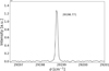 |
Fig. 2 Spectral line of the transition 5p z4F9/2 - 6s e4F9/2, with a typical signal-to-noise ratio and a FWHM of 0.109 cm−1. |
2.3 New energy levels
Combining the highly accurate energy levels belonging to the 4d25p configuration reported by Lawler et al. (2022) with wave numbers measured in this project, we derived new upper energy levels of the 4d26s and 4d25d configurations. Each energy level was derived as a weighted average of all measured transitions from that level. An example of this is seen in Table D.1 for the 4d26s e4F3/2 level, where seven transitions from the lower levels were identified and measured, resulting in a weighted mean energy of 59609.939 cm−1. Additional 4d25p and 4d5s5p levels were measured using transitions from the lower 4d25s and 4d3 levels reported by Lawler et al. (2022). These new 4d25p and 4d5s5p levels (see Table B.1) were in turn used to derive additional 4d26s and 4d25d levels. A complete list of the new 4d26s and 4d25d energies is presented in Table C.1.
The uncertainty in the new energy levels, where several lines are included, was estimated as the weighted standard deviation of the individual energy values. A conservative minimum of 0.001 cm−1 was used for the resulting energy levels.
2.4 Branching fractions
The BF for a line between two levels, u and l, is defined as
 (2)
(2)
where Aul is the transition probability of the targeted transition and the denominator is the sum of all transition probabilities (Auj) for transitions from the same upper level, u. For optically thin lines, Aul is proportional to the emitted intensity (Iul), since Iul ∝ NuguAul, where Nu is the population in the upper level and gu is its statistical weight. Thus, the BF for a transition is related to the relative intensities:
 (3)
(3)
Assuming that all lines have been measured, ***(eq4)*** . However, in practice, some lines may fall outside the spectral region covered by the instrument or are too weak to measure. The contribution from these missing lines must be estimated and accounted for in what is called the ‘residual’. A typical way of estimating this residual is using theoretical calculations, where BFs from all lines from a certain upper level are included. The residuals presented in Table E.1 were estimated from the results of the theoretical calculations introduced in Section 3.
For lines with a large transition probability and a highly populated lower level, the emitted light can be re-absorbed by another atom in the same lower state. This phenomenon is called self-absorption. Its probability depends on the ion density in the plasma, where a high ion density is obtained by increasing the current through the cathode. If self-absorption is present, the measured line intensity will appear lower for strong lines and thus would not correspond to the true intensity of the line. In such a case, a correction for this would be needed. The spectra used in this analysis are the same as those used in the study by Ljung et al. (2006). In their study, some of the 5s-5p lines exhibited self-absorption with a decrease in intensity of about 10% at the highest current, while others showed no apparent self-absorption. The Boltzmann population in the 5p levels is expected to be <1% of that of the 5s levels, even for temperatures higher than that typically found inside the HCL. This is confirmed by the fact that lines to 5p are much weaker than lines to 5s. Consequently, since the f-values of the stronger lines in this study are of the same order of magnitude as those found in Ljung et al. (2006), a self-absorption of ≪1% is to be expected for the lines presented in Table E.1. Compared to other sources of uncertainty presented in this analysis, the contribution of self-absorption is therefore negligible.
2.4.1 Intensity measurements
The main broadening mechanism in the HCL stems from the thermal motions of the light-emitting atoms and ions in the plasma and is referred to as thermal Doppler broadening. As a result, the spectral lines adopt a Gaussian line profile. Another broadening mechanism that also plays a role in the HCL is pressure broadening, which gives rise to a Lorentzian distribution. However, the effect of this is much less pronounced than Doppler broadening, which we tested by fitting both Gaussian and Voigt (convolution of a Gaussian and a Lorentzian) profiles using GFit with no noticeable difference. The intensity of the lines in this experiment was hence measured as the integrated area of a Gaussian fit.
The detection efficiency of the FTS is wave-number dependent and can be represented by a response curve (see Figure 3). This can be obtained using either an external calibration lamp, with known spectral radiance, or accurately determined carrier gas line intensity ratios. For this experiment, we use the latter method, where known ratios of Ar I and Ar II lines suitable for intensity calibration are recommended in Whaling et al. (1993). The response curve, seen in Figure 3, was constructed by comparing argon line ratios measured in this experiment to those presented in Whaling et al. (1993). The data were then fitted with a fifth-degree polynomial used as the estimated response throughout the spectral region. The response at a certain wave number enters the derivation of the BF as a calibration factor, c = 1/response, to the measured intensity (I), such that the calibrated intensity becomes Ical = cI.
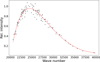 |
Fig. 3 Instrument response curve obtained using Ar I and II line ratios suggested by Whaling et al. (1993). |
2.4.2 Uncertainty in BF
The uncertainty in the BF of a line, ul, depends on the uncertainty in the measured intensity and in the calibration factor, cuj, of all lines involved, uj, from the same upper level. The total uncertainty in the BF of a line is thus estimated according to Sikström et al. (2002) as
 (4)
(4)
where I is the measured intensity and ∆I is the uncertainty in the Gaussian fit. The relative uncertainty in the calibration factor (∆c/c) is estimated from the standard deviation of the data points in Figure 3 relative to the fitted response curve. This is evaluated to be on average 7% along the curve. The derived relative uncertainties of the BFs, as shown in Table E.1, correlate with the intrinsic strengths of the lines, where the apparent weak lines tend towards higher uncertainties. For the lines that were not possible to measure, i.e. the residual, the uncertainty is included as a conservative 50%.
2.5 Lifetimes
The lifetimes were measured at the Lund High Power Laser Facility at Lund University using time-resolved laser-induced fluorescence (TR-LIF) in a two-step excitation scheme. The setup has been described in Lundberg et al. (2016), and an overview can be found in Figure 1 in Lundberg et al. (2016). Here, we only provide the most important details.
The free Zr+ ions were produced by laser ablation, where a frequency-doubled Nd:YAG laser (Continuum Surelite) with 10 ns pulses is focused on a rotating zirconium target placed in a vacuum chamber. The created plasma was then crossed by the two excitation lasers 0.5-1 cm above the target. The details of the two-step excitations are presented in Table A.1.
The first excitation step selectively reaches levels around 30000 cm−1 belonging to 4d2(3F)5p and is performed using a Nd:YAG laser (Continuum NY-82) pumping a Continuum Nd-60 dye laser giving 10 ns long frequency-doubled pulses. The selection of the final investigated 4d2 (3F)nl levels is achieved by the same type of lasers; however, here the Nd:YAG laser was injection-seeded, and the pulses were temporally compressed using stimulated Brillouin scattering in water. After frequency doubling in a KDP crystal or tripling in a BBO crystal, we obtained pulses with a typical temporal full width at half maximum (FWHM) of 1.2 ns.
The experiment was run at 10 Hz, and the timing of the three lasers was controlled by a delay generator, which allowed us to select the time between the plasma production and the excitation steps to optimise the signal. Furthermore, by controlling the time between the first 10 ns long excitation and the short 1 ns step, we could ensure that the second step occurs at the maximum population of the intermediate level.
Fluorescence from the excited states was detected perpendicular to the three laser beams, with a 1/8 m grating monochromator with a 0.28 mm wide entrance slit, resulting in a line width of 0.5 nm in the second spectral order. To optimise the light yield, the slit was oriented parallel to the excitation lasers. The light was finally detected by a fast microchannel-plate photomultiplier tube (Hamamatsu R3809U) and digitised by a Tektronix DPO 7254 oscilloscope triggered by the second-step laser pulses detected with a fast photodiode. The temporal shape of the laser pulse was also sampled on a second channel of the oscilloscope. Each measurement was averaged over 1000 laser pulses, and the resulting decay curve was analysed by fitting a single exponential convoluted by the measured second excitation pulse and a background function using the code DECFIT (Palmeri et al. 2008). An example of a recorded decay curve and the excitation laser is given in Figure 4. Whenever possible, the decay was measured in several different decay channels (Table A.1). For two levels, the fluorescence had to be measured at the same wavelength as the second step laser, leading to some perturbation from scattered laser light. This was corrected for by separately recording the scattered light with the first-step laser turned off and subtracting this signal from the measured decay curve before the final fitting procedure.
The resulting lifetimes are presented in Table A.1 and represent an average of at least ten measurements in each channel performed on different days. The variation of the repeated measurement was also used to estimate the uncertainty in the quoted lifetimes.
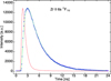 |
Fig. 4 Decay of the 6s 2F7/2 level in ZrII at 61835 cm−1 with a lifetime of 3.1 ns. The decay (blue) is plotted with plus (+) signs. The recorded laser pulse (red) and the fitted decay curve (green) are shown with solid lines. The actual measurement extends to 54 ns. |
2.6 log gf-values
Once the BFs of transitions from a certain upper level, u, are derived, they can, together with the lifetime of the upper level, τu, be used to determine the transition probability, according to
 (5)
(5)
For the purpose of astrophysical applications, such as elemental abundance analyses, the desired parameter is the oscillator strength, f. This value is related to the transition probability, such that
 (6)
(6)
where gu and gl are the statistical weights of the upper and lower levels, respectively, and λ is in nm. Note that Aul is the emission transition probability, whereas flu is the absorption oscillator strength. The uncertainty in the transition probability is derived from the uncertainty in the BFs and in the lifetimes. The estimated total uncertainty in the gf-values is given in Table E.1.
3 Calculations
The pseudo-relativistic Hartree-Fock (HFR) method developed by Cowan (1981) and modified to account for core polarisation effects - giving rise to the HFR+CPOL method (Quinet et al. 1999, 2002) - was used to calculate the level lifetimes and the BFs for the transitions depopulating the energy levels of interest in Zr II. In the present work, the physical model used was based on the consideration of three valence electrons surrounding a Kr-like Zr V ionic core made of 36 electrons filling the so-called core orbitals from 1s to 4p.
Therefore, the correlations between valence electrons were evaluated in a configuration interaction scheme by explicitly including the following configurations in the calculations: 4d25s + 4d26s + 4d27s + 4d25d + 4d26d + 4d27d + 4d3 + 4d5s2 + 4d5p2 + 4d5d2 + 4d4f2 + 4d5f2 + 4d5s6s + 4d5s5d + 4d5s6d + 4d5p4f + 4d5p5f + 5s26s + 5s25d + 5s26d (even parity) and 4d25p + 4d26p + 4d27p + 4d24f + 4d25f + 4d5s5p + 4d5s6p + 4d5s4f + 4d5s5f + 4d5p5d + 4d5d4f + 4d5d5f + 5s25p + 5s26p + 5s24f + 5s25f (odd parity). The core-valence correlations were then estimated using a core polarisation potential. Here, the dipole polarisability of the ionic core, αd, was set to 2.98 a03, as reported in Johnson et al. (1983) for Zr V. Moreover, the cutoff radius, rc, was set to 1.35 a0, which corresponds to the average value 〈r〉 for the outermost core orbital (4p) obtained in our HFR calculations.
Using the experimental levels reported by Kiess & Kiess (1930) and Lawler et al. (2022), supplemented by the experimental values measured in the present work (see Tables B.1-C.1), some radial parameters, such as average energies (Eav), Slater integrals (Fk, Gk), spin-orbit parameters (ζnl), and effective interaction parameters (α, β) belonging to the 4d25s, 4d26s, 4d25d, 4d3, 4d5s2, 4d5p2, and 4d5s6s even-parity configurations as well as the 4d25p and 4d5s5p odd-parity configurations were adjusted using a well-established semi-empirical procedure (Cowan 1981). This led to mean standard deviations between calculated and experimental energy levels equal to 240 cm−1 and 92 cm−1 for the even- and odd-parity levels, respectively. The computed radiative lifetimes are presented together with the experimental values in Table A.1 and the BFs and oscillator strengths in Table E.1.
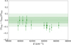 |
Fig. 5 Comparison between experimental and calculated lifetimes for the 13 first levels in Table A.1. The error bars correspond to the uncertainty in the experimental results. The shaded areas show the 5 and 10% deviation. |
4 Results and discussion
We report the energies of 34 levels belonging to the 4d25p, 4d5s5p, 4d25d, and 4d26s configurations. The odd-parity levels (4d25p and 4d5s5p), presented in Table B.1, differ with a weighted average of 0.039 cm−1 and a standard deviation of 0.113 cm−1 from the earlier work by Kiess & Kiess (1930). The evenparity high-excitation levels (4d25d, 4d2 6s), listed in Table C.1, have not been reported before. We also note that none of the 4d26s levels in Kiess & Kiess (1930) could be verified. However, we confirm all levels belonging to the 4d25s, 4d3, 4d5s2, 4d25p, and 4d5s5p configurations.
For the even-parity high-excitation levels, we present new radiative lifetimes in Table A.1, together with the experimental uncertainties. In Table E.1, we report air wavelengths (λair), BFs, and log gf values for 79 transitions coming from 13 of the measured even-parity high-excitation levels.
A comparison between our computed and experimental lifetimes (Table A.1) shows good agreement with a mean ratio of τcalc/τexp = 1.09 ± 0.24. This is further illustrated in Figure 5, where the computed and measured lifetimes for the first 13 levels show an overall agreement of 10%. In Table E.1, the HFR+CPOL-calculated BF and log gf-values are compared with the experimental values. The average deviation is approximately 25% for both BF- and g f -values, indicating a good level of agreement. For the log g f -values, we see in Figure 6 that most theoretical values lie within 0.1 dex of the experimental ones, with an average difference of 0.04 dex. However, we see a wider spread as well as larger uncertainties at lower log g f -values. This is due to weaker lines being more difficult to both experimentally measure and theoretically calculate, giving rise to larger possible discrepancies between the two methods.
The last six levels listed in Table A.1 remain without spectroscopic designations due to the difficulty in assigning them unambiguously, both experimentally and in the HFR+CPOL calculations. Theoretically, we find that several configurations, such as 4d5p2, 4d25d, 4d5s6s, and 4d5s5d, are strongly mixed above 75 000 cm−1. It is interesting to note that, while the average LS-coupling purity of the even levels below 75 000 cm−1 is about 80% in the HFR+CPOL calculations, it drops to 60% for the levels between 75 000 and 80 000 cm−1. Furthermore, these levels are not included in Table E.1 since a reliable BF analysis could not be done due to the difficulty in theoretically estimating the residual.
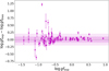 |
Fig. 6 Comparison between experimental and calculated log g f values for lines from all levels included in Table 5. The error bars correspond to the uncertainty in the experimental results. The shaded areas show a ±0.1 and 0.2 dex difference. |
5 Conclusions
This paper provides an extended understanding of the spectrum of singly ionised zirconium for highly excited levels. We presented experimental energies, experimental and theoretical lifetimes, as well as log g f -values. The two methods show good agreement in the log gf values for the stronger lines and a larger deviation for the weaker lines. For further astrophysical investigations, we recommend using the experimental values of the log g f.
Acknowledgements
The research leading to these results has received funding from LASERLAB-EUROPE (grant agreement no. 654148, EU H2020), the Belgian F.R.S.-FNRS, the Swedish Research Council Grants 2016-04185 and 2023-05367, the Carl Trygger Foundation, and the Krapperup Foundation. P.P. and P.Q. are respectively Research Associate and Research Director of the Belgian Fund for Scientific Research F.R.S.-FNRS.
References
- Biemont, E., Grevesse, N., Hannaford, P., & Lowe, R. M. 1981, ApJ, 248, 867 [Google Scholar]
- Cowan, R. D. 1981, The Theory of Atomic Structure and Spectra (California, USA: University of California Press) [Google Scholar]
- Engström, L. 1998, Lund reports on atomic physics [Google Scholar]
- Forsberg, R., Jönsson, H., Ryde, N., & Matteucci, F. 2019, A&A, 631, A113 [NASA ADS] [CrossRef] [EDP Sciences] [Google Scholar]
- Froese-Fischer, C., Brage, T., & Jönsson, P. 1997, Computational Atomic Structure: An MCHF Approach, 1st edn. (Bristol and Philadelphia: Institute of Physics Publishing) [Google Scholar]
- Johnson, W. R., Kolb, D., & Huang, K. N. 1983, Atomic Data Nucl. Data Tables, 28, 333 [Google Scholar]
- Kiess, C. C., & Kiess, H. K. 1930, J. Res. Natl. Bureau Standards, 5, 1205 [Google Scholar]
- Langhans, G., Schade, W., & Helbig, V. 1995, Zeitschrift fur Physik D Atoms Molecules Clusters, 34, 151 [Google Scholar]
- Lawler, J., Schmidt, J., & Hartog, E. A. D. 2022, J. Quant. Spectr. Rad. Transf., 289, 108283 [Google Scholar]
- Learner, R. C. M., & Thorne, A. P. 1988, J. Opt. Soc. Am. B Opt. Phys., 5, 2045 [NASA ADS] [CrossRef] [Google Scholar]
- Liggins, F. S., Pickering, J. C., Nave, G., et al. 2021, ApJ, 907, 69 [Google Scholar]
- Ljung, G., Nilsson, H., Asplund, M., & Johansson, S. 2006, A&A, 456, 1181 [NASA ADS] [CrossRef] [EDP Sciences] [Google Scholar]
- Lundberg, H., Hartman, H., Engström, L., et al. 2016, MNRAS, 460, 356 [Google Scholar]
- Malcheva, G., Blagoev, K., Mayo, R., et al. 2006, MNRAS, 367, 754 [Google Scholar]
- Molero, M., Magrini, L., Matteucci, F., et al. 2023, MNRAS, 523, 2974 [NASA ADS] [CrossRef] [Google Scholar]
- Moore, C. E. 1952, Atomic Energy Levels, as Derived from the Analyses of Optical Spectra (USA: National Standard Reference Data Series, National Bureau of Standards), 2 [Google Scholar]
- Nave, G., Sansonetti, C. J., & Griesmann, U. 1997, in Fourier Transform Spectroscopy (USA: Optica Publishing Group), FMC.3 [Google Scholar]
- Palmeri, P., Quinet, P., Fivet, V., et al. 2008, Phys. Scr, 78, 015304 [Google Scholar]
- Peck, E. R., & Reeder, K. 1972, J. Opt. Soc. Am., (1917-1983), 958 [Google Scholar]
- Quinet, P., Palmeri, P., Biémont, E., et al. 1999, MNRAS, 307, 934 [NASA ADS] [CrossRef] [Google Scholar]
- Quinet, P., Palmeri, P., Biémont, E., et al. 2002, J. Alloys Compounds, 344, 255 [CrossRef] [Google Scholar]
- Salit, M. L., Travis, J. C., & Winchester, M. R. 1996, Appl. Opt., 35, 2960 [Google Scholar]
- Sikström, C. M., Lundberg, H., Wahlgren, G. M., et al. 1999, A&A, 343, 297 [NASA ADS] [Google Scholar]
- Sikström, C. M., Nilsson, H., Litzén, U., Blom, A., & Lundberg, H. 2002, J. Quant. Spec. Radiat. Transf., 74, 355 [CrossRef] [Google Scholar]
- Travaglio, C., Gallino, R., Arnone, E., et al. 2004, ApJ, 601, 864 [Google Scholar]
- Whaling, W., Carle, M. T., & Pitt, M. L. 1993, J. Quant. Spec. Radiat. Transf., 50, 7 [Google Scholar]
Appendix A Lifetimes
Two-step excitation schemes in Zr II.
Appendix B Odd-parity energy levels
Odd-parity levels in ZrII.
Appendix C Even-parity energy levels
New even-parity energy levels in Zr II.
Appendix D Identification of new level
Identification of the new 4d2(3F)6s e4F3/2 level at 59609.933 cm−1.
Appendix E Transition data
Wavelengths, transition probabilities, and log gf in Zr II.
All Tables
All Figures
|
Fig. 1 Partial energy level diagram of Zr II. |
| In the text | |
|
Fig. 2 Spectral line of the transition 5p z4F9/2 - 6s e4F9/2, with a typical signal-to-noise ratio and a FWHM of 0.109 cm−1. |
| In the text | |
|
Fig. 3 Instrument response curve obtained using Ar I and II line ratios suggested by Whaling et al. (1993). |
| In the text | |
|
Fig. 4 Decay of the 6s 2F7/2 level in ZrII at 61835 cm−1 with a lifetime of 3.1 ns. The decay (blue) is plotted with plus (+) signs. The recorded laser pulse (red) and the fitted decay curve (green) are shown with solid lines. The actual measurement extends to 54 ns. |
| In the text | |
|
Fig. 5 Comparison between experimental and calculated lifetimes for the 13 first levels in Table A.1. The error bars correspond to the uncertainty in the experimental results. The shaded areas show the 5 and 10% deviation. |
| In the text | |
|
Fig. 6 Comparison between experimental and calculated log g f values for lines from all levels included in Table 5. The error bars correspond to the uncertainty in the experimental results. The shaded areas show a ±0.1 and 0.2 dex difference. |
| In the text | |
Current usage metrics show cumulative count of Article Views (full-text article views including HTML views, PDF and ePub downloads, according to the available data) and Abstracts Views on Vision4Press platform.
Data correspond to usage on the plateform after 2015. The current usage metrics is available 48-96 hours after online publication and is updated daily on week days.
Initial download of the metrics may take a while.