| Issue |
A&A
Volume 705, January 2026
|
|
|---|---|---|
| Article Number | A188 | |
| Number of page(s) | 7 | |
| Section | The Sun and the Heliosphere | |
| DOI | https://doi.org/10.1051/0004-6361/202557395 | |
| Published online | 20 January 2026 | |
Estimating the cross-sectional sizes of potential solar triggers of near-Sun magnetic switchbacks
Physics Department University of Ioannina 45110, Greece
★ Corresponding author: This email address is being protected from spambots. You need JavaScript enabled to view it.
Received:
24
September
2025
Accepted:
24
November
2025
Abstract
Context. The discovery of near-Sun magnetic switchbacks (SBs) represents a key result of the Parker Solar Probe (PSP) mission.
Aims. Several theories and models suggest that near-Sun SBs may be triggered by small-scale transient phenomena occurring in the low solar atmosphere. Therefore, estimating the cross-sectional sizes of potential triggers that are consistent with near-Sun SB observations could place tighter constraints on related theories and models.
Methods. We propose a simple method based on the conservation of magnetic flux in flux tubes connecting near-Sun SBs with their potential triggers in the low solar atmosphere. This method combines inferences of SB diameters and their magnetic fields from PSP in situ observations and estimates of the low-solar atmosphere magnetic fields, calculated at heights pertinent to proposed solar triggers of near-Sun SBs, from magnetic field extrapolations in areas on the Sun that are magnetically connected with PSP. The application of our method provides estimates of the radii of the cross-sections of potential near-Sun SB triggers taking place in the low solar atmosphere.
Results. We applied our method to the SBs observed during the first solar encounter of PSP, when the spacecraft was connected to a small equatorial coronal hole. The inferred radii of the cross-sections of potential triggers of near-Sun SBs in the low solar atmosphere take values in the range ≈10–26 000 km; a more compressed range of ≈125–3500 km corresponds to the most representative SB diameters values.
Conclusions. The latter range of potential solar near-Sun SB trigger radii is fully accessible by contemporary extreme UV (EUV) and UV instrumentation, with its lowest end of around 125 km being reachable by the Extreme Ultraviolet Imager on board the Solar Orbiter mission. This range is also consistent with the spatial scales of proposed near-Sun SB triggers in the low solar atmosphere. The smallest SB diameters we considered give rise to potential near-Sun SB solar trigger radii below ≈100 km, which are inaccessible with current EUV and UV instrumentation. Given that the inferred cross-sections sizes of the potential solar triggers of near-Sun SBs are significantly smaller than the respective errors in establishing their actual locations via magnetic connectivity tools, it is more appropriate to compare statistics of near-Sun SBs and their potential solar triggers on scales commensurate with the cross-sections inferred here, rather than with the entire connected region for encounter 1. Our simple method, paired with magnetic connectivity studies, is a step towards more refined assessments of potential solar triggers of near-Sun SBs.
Key words: Sun: atmosphere / solar wind
© The Authors 2026
 Open Access article, published by EDP Sciences, under the terms of the Creative Commons Attribution License (https://creativecommons.org/licenses/by/4.0), which permits unrestricted use, distribution, and reproduction in any medium, provided the original work is properly cited.
This article is published in open access under the Subscribe to Open model. This email address is being protected from spambots. You need JavaScript enabled to view it. to support open access publication.
1. Introduction
One of the most important discoveries of the Parker Solar Probe (PSP) mission (Fox et al. 2016) is the prevalence of magnetic switchbacks (SBs) in the near-Sun environment (Bale et al. 2019; Kasper et al. 2019), a region explored with in situ observations for the first time with PSP. In essence, SBs correspond to transient and sizeable deflections in the direction of the interplanetary magnetic field (IMF), which are, however, not associated with crossings of the heliospheric current sheet (e.g. Bale et al. 2019; Kasper et al. 2019). The near-Sun SBs discovered by PSP have a duration ranging from a few seconds to a few hours (e.g. Dudok de Wit et al. 2020). Near-Sun SBs could be important suppliers of the heating and acceleration of the young solar wind (e.g. Akhavan-Tafti et al. 2022). For a review of SB properties, the interested reader can consult Raouafi et al. (2023a) and Velli & Dudok de Wit (2026). Additionally, SBs have been observed within the inner heliosphere by, for example, Ulyssess and HELIOS (Balogh et al. 1999; Horbury et al. 2018) and more recently by Solar Orbiter (e.g. Fedorov et al. 2021); PSP observations demonstrate that SBs can also be detected much closer to the Sun.
The discovery of near-Sun SBs has generated significant interest in their possible triggers (e.g. the review of Raouafi et al. 2023a). Several works involve solar triggers of near-Sun SBs (e.g. Sterling & Moore 2020; Tenerani et al. 2020; Fargette et al. 2021; Drake et al. 2021; de Pablos et al. 2022; Upendran & Tripathi 2022; Wyper et al. 2022; Kumar et al. 2022; Biondo et al. 2023; Huang et al. 2023a,b; Raouafi et al. 2023b; Hou et al. 2024b; Touresse et al. 2024; Hou et al. 2024a; Bizien et al. 2025; Hou et al. 2025; Lee et al. 2025). According to these studies, potential solar triggers of near-Sun SBs include transient phenomena occurring in the low solar atmosphere, such as interchange reconnection in the chromospheric network boundaries at the base of the transition region and transient mass outflows in the form of jets of various scales. Tripathi et al. (2026) provides a complete review of the potential solar triggers of near-Sun SBs.
Connecting phenomena and physical conditions in the solar wind with their potential solar sources is achieved by joint solar remote-sensing and in situ solar wind observations (e.g. Yardley et al. 2024). A basic element of these studies is to establish the magnetic connectivity between the in situ monitor and the Sun (e.g. the review of Rouillard et al. 2020). This is achieved by data-constrained modelling, which includes global solar magnetic field models, magnetic field measurements, and assimilation in the Sun and solar wind speed measurements. This is essentially a back-mapping procedure, going from the spacecraft to its magnetic footpoint on the solar surface, and typically consists of two steps (see Fig. 1 in Koukras et al. (2025). The first step involves ballistic propagation along the Parker spiral (Parker 1958) from the spacecraft to the source-surface of the global magnetic field1. In the second step, magnetic coupling from the source-surface to the solar surface is achieved by tracing magnetic field lines of a global magnetic field model. The end result of back-mapping procedures is to supply the location, i.e. the magnetic footpoint, on the solar surface to which the magnetic field line from a specific spacecraft in the near-Sun environment or heliosphere is connected. Fig. 1a presents a simple schematic of the point mapping for a near-Sun SB. The associated uncertainty in determining the magnetic footpoint locations can amount to several degrees on the Sun (e.g. Koukras et al. 2025); therefore, magnetic connectivity studies identify, at best, a specific (extended) solar connected area (e.g. quiet Sun, coronal hole, or active region).
 |
Fig. 1. Simple schematic of SB-Sun magnetic connectivity. (a) Point connectivity: a near-Sun SB recorded at point PSB is magnetically connected to point Psol on the Sun or in the low solar atmosphere (blue ‘X’). The derived solar connection point has significant uncertainty (dashed circle). (b) Area connectivity: a near-Sun SB with a cross-sectional area ASB is mapped to an area Asol in the low solar atmosphere, where a potential SB trigger operates, via the flux tube passing between these two areas. Both plots are not to scale and do not consider the Parker spiral. |
Recent studies connecting SBs with their potential solar triggers include de Pablos et al. (2022), Huang et al. (2023b), Kumar et al. (2023), Hou et al. (2024a,b), Bizien et al. (2025). These studies employed magnetic connectivity tools to pinpoint the solar region that was magnetically connected to PSP during the studied SB intervals. They then compare the observed SB statistics (e.g. numbers or rates) with various observed parameters of the associated magnetically connected solar regions (e.g. numbers and rates of coronal jets or light curves).
For extended in situ features such as SBs, which have a finite spatial extend and duration, we can investigate the regions on the Sun or in the low solar atmosphere to which the studied SBs are mapped. This can be particularly helpful for testing solar SB triggers. Consider a flux tube encapsulating a near-Sun SB (see Fig. 1b) If the SB has a cross-sectional area ASB, then we determine the cross-sectional area, Asol, of the SB flux tube in the low solar atmosphere. The value of Asol corresponds to the height(s) at which a given SB solar trigger operates. This implies that each time an SB is observed, it corresponds to a single flux tube as depicted in in situ observations of distinct SBs.
Therefore, establishing constraints on the sizes of the cross-sections in the low solar atmosphere of flux tubes connecting to near-Sun SBs will provide further insights and guidance for testing their potential solar origins. This is the focus of our investigation. In Sect. 2 we present a simple method to estimate the cross-section size of the solar triggers of near-Sun SBs; Sect. 3 presents an application of our method to the first solar encounter of PSP; and Sect. 3.1 contains a summary and discussion of our results.
2. Simple method to estimate SB flux tube cross-sectional size
Our method for inferring the cross-sectional sizes of potential solar triggers of near-Sun SBs is based on the conservation of the magnetic flux in flux tubes connecting the near-Sun SBs to their solar triggers (see Fig. 1b). Assuming circular cross-sections of these flux tubes, the SB solar trigger radius, rsol, is given by
 (1)
(1)
where rSB is the SB radius, and Bsol and BSB are the magnitudes of the solar trigger and the SB radial magnetic field, respectively. Equation (1) implicitly assumes that the low-solar-atmosphere SB trigger(s) operate on cross-sections with radius rsol. In turn, rsol is determined by the cross-field spatial scale of the postulated solar trigger, which, for example, could correspond to the base of jets. For SBs with circular cross-sections and diameter wSB, rSB = 0.5wSB. From Eq. (1), we note that rsol has a weak square-root dependence on BSB and Bsol, which significantly absorbs uncertainties in both parameters. In calculating rsol from Eq. (1), we used in situ measurements and estimates of BSB and rSB, respectively. For Bsol in the low solar atmosphere above the photospheric layer, we used magnetic field extrapolations in the solar area that is magnetically connected to PSP during the studied SB intervals.
3. Application to PSP encounter 1
We applied our methodology to the first solar encounter of PSP, which took place between 30 October and 13 November 2018, when PSP flew in the near-Sun environment, reaching heliocentric distances from 36 to 54 R⊙. During this interval, PSP quasi-corotated with the Sun. The magnetic footpoint of PSP from the magnetic field line connecting PSP to the Sun (as determined from magnetic connectivity assessments), was confined within a small equatorial coronal hole (ECH) (Bale et al. 2019; Badman et al. 2020; de Pablos et al. 2022; Wallace et al. 2022). Therefore, during this interval, PSP was magnetically connected to this small ECH. Small drifts of the PSP magnetic footpoint within the ECH occurred during this interval (see, e.g. Fig. 1d in Bale et al. 2019 and Fig. 4 in Wallace et al. 2022). SBs were prominently observed during PSP encounter 1 (e.g. Bale et al. 2019; Kasper et al. 2019).
3.1. SB parameters
During PSP encounter 1, BSB, took values from the interval ≈20–90 nT (see, e.g. Fig. 1a in Bale et al. 2019). In our implementation of Equation (1), we considered 30 uniformly distributed values of BSB within this interval. Because we focus on near-Sun SBs, the angle between the Parker spiral and the radial is small, i.e. not exceeding 16 degrees for a median solar wind speed of ≈350 km/s during PSP encounter 1, so attributing the radial component of the IMF to the near-Sun SB cross-sections is well justified.
For wSB, and therefore rSB, we note that using the SB duration, that is, the time the PSP spends inside a given SB, could be insufficient by itself to provide an accurate estimate of wSB. This is because we are considering single-spacecraft observations, and the SB duration depends on both the SB shape and how the PSP trajectory intersects each SB. Several studies report a wide range of values for SBs observed during PSP encounter 1. Laker et al. (2021), following earlier work by Horbury et al. (2020), based their analysis on the assumption that SBs correspond to long, thin cylinders. They developed a model employing the average switchback width and aspect ratio as free parameters, which was fitted to the distribution of switchback durations for various spacecraft cutting angles. The optimal cutting angles were chosen as those consistent with long, thin cylinders. Their fittings yield average SB diameters of 33 000, 50 000, and 89 000 km for several solar wind streams permeated with SBs during encounter 1; a total of 239 SBs were observed (see their Table A.1.). Larosa et al. (2021) estimated wSB by considering the proton velocity along the normal direction at the leading and trailing edge boundary, as well as the duration of a set of 70 SBs with sharp boundaries. They deduced SB boundary normal directions using the minimum variance analysis (MVA) method. From their Fig. 6, the peak of the associated distribution is around 6 × 10⁴ km and the associated range of values corresponding to more than 10% of the distribution peak is ≈4 × 10³ − 3 × 10⁵ km. Meng et al. (2022) also applied the MVA method, assuming cylindrical SBs, to in situ magnetic field measurements of 129 SBs. The distribution of the resulting values is broad and somewhat non-smooth (+(see their Fig. 5). The peak of their wSB distribution is around 1.5 ×10⁵ km, and the wSB range for values above 10% of the associated distribution peak is ≈2.5 × 10³ − 6.5 × 10⁵ km. The MVA method can encounter issues when calculating the normal vectors to SB boundaries, as shown in Bizien et al. (2023). This may partially explain the wider distributions of wSB obtained using the MVA method. Another factor is that MVA-based methods calculate wSB for individual SBs, whereas Laker et al. (2021) deduce wSB for an ‘average’ SB per studied solar wind stream. Given these considerations, the wSB range reported by Laker et al. (2021), spanning 33 000–89 000 km, may be regarded as the most representative for PSP encounter 1. This range is, however, partially covered by the more extended ranges reported by Larosa et al. (2021) and Meng et al. (2022). We nevertheless considered the following five wSB values: 2500, 33 000, 15 000, 89 000, and 650 000 km. These values encompass the full range of pertinent values discussed above and span two orders of magnitude.
3.2. Solar parameters
To estimate Bsol, we used a co-temporal Atmospheric Imaging Assembly (AIA) (Lemen et al. 2012) 193 Å image and a Helioseismic and Magnetic Imager (HMI) (Scherrer et al. 2012) 720-s full-disc line-of-sight (LoS) photospheric magnetogram pair, taken around 06:00:00 UT on 28 October 2018. This snapshot was close in time to the central meridian passage of the small ECH, which was magnetically connected to PSP during encounter 1. Selecting this snapshot provides the best vantage point of the ECH photospheric magnetic field, which is less prone to projection effects. We first trimmed the EUV image and LoS magnetogram over a field of view that encompasses the small ECH. We then manually outlined the ECH boundary in the 193 Å image and generated a binary mask with a value of 1 for pixels inside the ECH and 0 for those outside. ECHs are prominently observed in 193 Å channel (e.g. Hofmeister et al. 2017). For the selected snapshot, the absolute mean magnetic field density of the ECH is 1.5 G, a value within the bulk of the distribution of respective values from the statistical survey of Hofmeister et al. (2017), who analysed AIA 193 Å and HMI observations of 288 ECHs. They report an absolute mean magnetic field density of 3 ± 1.6 G (see also their Figure 4c). The percentage of unbalanced magnetic flux (ratio of net unsigned to net signed magnetic flux) is 23%, which lies within the range of 6–81% reported by Hofmeister et al. (2017).
We next extrapolated the radialised LoS photospheric magnetic field, i.e. we converted the LoS magnetic field to radial assuming a purely radial magnetic field. We used the Fourier-transform-based method of Alissandrakis (1981), under the assumption of a potential, i.e. current-free, magnetic field. A potential field is the simplest approximation used in magnetic field extrapolations and is frequently employed in ECH studies (e.g. Kumar et al. 2019).
In our rsol calculations using Equation-(1), we assigned the unsigned Bz values, resulting from the potential extrapolation for various considered height ranges and for the area bounded by the ECH mask, to Bsol. The choice of these height ranges is motivated by the discussion of potential solar triggers of SBs in the Introduction. Coronal bright points (CBPs) (e.g. Madjarska 2019) are frequently found at the bases of coronal jets (e.g. Raouafi et al. 2016 and essentially determine their starting height. Observations of CBPs at 1 MK temperatures give rise to heights between 5 and 10 Mm Madjarska (2019). Bale et al. (2021, 2023) suggest that interchange reconnection may occur just above the transition region. A compilation of various observations suggests that the base of the transition region is around 2.5–3.5 Mm (Alissandrakis 2023). Finally, campfires reach heights of 1–5 Mm (Zhukov et al. 2021). Campfires (Berghmans et al. 2021) are the smallest-scale and most numerous EUV brightenings detected to date, which are frequently associated with small-scale jets (e.g. Hou et al. 2021).
3.3. Results
For each considered wSB value, and from application of Equation (1), we calculated the respective rsol values for all combinations of the Bsol values per considered height range, within the manually traced ECH boundary and the respective BSB values. Figure 1 shows histograms of the resulting rsol values for SB triggers within the 5–10 Mm height range, and Table 1 contains the fifth, 50th, and 95th percentile values of the respective rsol distributions for each considered wSB. Larger wSB values typically lead to larger rsol. The fifth percentile rsol values generally correspond to the larger Bsol values, and hence to locations of enhanced magnetic fields in the low solar atmosphere.
Percentile values of cross-sectional radii (km) for solar SB triggers in the height range 5–10 Mm and for different wSB values.
Tables 2 and 3 contain the fifth, 50th, and 95th percentile values of rsol for SB trigger heights of 2.5–3.5 and 1–5 Mm, respectively. We note that the entries in Tables 2 and 3 were obtained independently. Comparison of the corresponding rows, i.e. supplying the fifth, 50th, and 95th percentile values of rsol for a given wSB, in Tables 1–3 suggests that considering different SB trigger height ranges has a rather small impact on the resulting rsol. However, the 1–5 Mm height range gives rise to a somewhat smaller rsol than the other two height ranges used. Overall, rsol takes values from ≈10–26 000 km, while considering the most representative range of wSB values (second and third rows of Tables 1–3) gives rise to rsol from ≈125–3500 km.
4. Discussion and conclusions
Establishing estimates of the cross-sectional areas of potential triggers of near-Sun SBs in the low solar atmosphere will allow more scrutiny of pertinent models and theories. In this study, we used a simple method to infer the radii of potential near-Sun SB triggers in the low solar atmosphere for PSP encounter 1. The method is based on magnetic flux conservation in flux tubes connecting near-Sun SBs with their potential triggers in the low solar atmosphere. It employs SB in situ magnetic field observations and inferences of their diameters, along with imaging and magnetic field observations and extrapolations pertinent to the solar area that is magnetically connected with PSP during the studied interval of near-Sun SBs.
Our conclusions are summarised as follows:
-
The value of rsol varies significantly between ≈10–26 000 km.
-
The most representative wSB measurements give rise to a more compressed rsol range of ≈125–3500 km.
-
The exact height range considered in the low solar atmosphere of potential SB triggers has a minimal impact on the resulting rsol values.
The resulting rsol values for the most representative wSB measurements (blue and red histograms of Fig. 3) are accessible with our current EUV and UV instrumentation observing the low solar atmosphere, including AIA (Scherrer et al. 2012), the Interface Region Imaging Spectrograph (IRIS; De Pontieu et al. 2014) and the Extreme Ultraviolet Imager (EUI; Rouillard et al. 2020) on board the Solar Orbiter Mission (Müller et al. 2020) (see the shaded area in Fig. 3). Moreover, the resulting rsol values are consistent with the spatial scales of various transient phenomena occurring in the low solar atmosphere, e.g. CBPs, coronal jets, and campfires, which, as discussed in Section 3.2, are proposed triggers of near-Sun SBs. The low end of the resulting rsol values, of the order of 125 km, can be resolved by EUI. Therefore, applying our framework to other PSP encounters, with Solar Orbiter EUI coverage of the magnetically connected regions with PSP, may help to better assess the validity of proposed solar triggers of near-Sun SBs. The upper end of the resulting rsol distribution of ≈260 000 km is close to the spatial scale of supergranulation. In addition, our rsol values also span the spatial scales of granulation (≈10 000 km). These results are consistent with SB observations showing modulations in their occurrence, i.e. SB patches, at scales commensurate with those of granulation and supergranulation (e.g. Bale et al. 2021; Fargette et al. 2021; Bale et al. 2023).
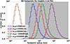 |
Fig. 3. Histograms of rsol for wSB equal to 2500, 33 000, 89 000, 150 000, and 650 000 km, shown as brown, blue, green, red, and purple lines, respectively, for an SB trigger in the height range 5–10 Mm. The grey-shaded area encapsulates rsol values accessible with our existing EUV instrumentation; the smallest rsol in this area can be measured by the Extreme Ultraviolet Imager on board Solar Orbiter. |
The resulting rsol range for the largest considered wSB (purple histogram of Fig. 3), is also accessible with current EUV and UV instrumentation. In contrast, the rsol values for the smallest considered wSB (brown histogram of Fig. 3), correspond to scales below ≈100 km, which are currently not resolvable with our EUV and UV instrumentation observing the low solar atmosphere.
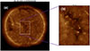 |
Fig. 2. Panel (a): Full-disc AIA 193 Å image taken at 06:00:04 on 28 October 2018, around the central meridian passage of an ECH magnetically connected to PSP during its first solar encounter. The ECH is bounded by the rectangular box. Panel (b): Sub-image of the AIA 193 Å image of panel (a), corresponding to the rectangular box in panel (a). The manually-selected ECH boundary is over-plotted with dashed green lines. |
The resulting rsol values are also significantly smaller than the total area of the ECH that was magnetically connected with the PSP during encounter 1, spanning ≈500 × 640 arcsec2 (i.e. the size of the box in Fig. 2). Therefore, SB counting statistics during a studied interval need to be compared with the average number of occurrences of potential solar triggers of SBs over areas of rsol radii, rather than with their occurrences over the entire magnetically connected region, namely, the ECH of Fig. 2. In other words, this essentially calls for statistical assessments that combine SB statistics with solar statistics over an array of sliding windows with rsol radii scanning the entire connected region. Moreover, the resulting rsol values are also significantly smaller than the uncertainty in determining the location of the SB footpoints on the Sun. This implies that it is not meaningful to attempt one-to-one associations between areas with rsol radii centred at the magnetic footpoints of SBs and individual SBs.
Our calculations of rsol focus on three height ranges of potential near-Sun SB triggers. These ranges are representative of several basic scenarios of near-Sun SB triggers but do not include all possibilities. However, our results suggest that rsol values have a rather weak dependence on the choice of the height range.
Using a PFSS extrapolation from a synoptic map of the photospheric magnetic field leads to smaller rsol values than our potential extrapolation, but still spanning a few hundred km for the most representative range of wSB values (see Appendix A). Because our study focusses on small-scale transient solar phenomena that may trigger near-Sun SBs, we consider magnetic extrapolations with the highest applicable spatial resolution, such as the potential magnetic field extrapolation of Section 2, to be the more suitable approach. We also note that a more complex magnetic extrapolation model, such as the non-linear-force-field (NLFF) model requires the full photospheric magnetic field vector, and its horizontal components are predominately dominated by noise in weak-field regions such ECHs in HMI observations. Moreover, Liu et al. (2011) compared a potential and three NLFF extrapolations over a quiet Sun region using Hinode Solar Optical Telescope observations and found very small differences of the order of 0.1 Gauss, between the potential and NLFF extrapolations for heights 2000 km above the photosphere. In summary, a potential magnetic field extrapolation is deemed a reasonable choice for the purposes of our exploratory study.
The ratio of the SB flux-tube area at PSP to that in the low solar atmosphere, for example, considering the most probable rsol values and the respective wSB values (first and third columns of Tables 1–3), takes values in the range ≈1800–2300. This is about 1.5 larger than the areal expansion anticipated from a purely radial expansion,  , where 35 R⊙ corresponds to the perihelion distance of PSP during its first encounter. This result is consistent with the small magnetic expansion factors in coronal holes in general (Wang & Sheeley 1990) and also with the ECH of encounter 1 in particular (Stansby et al. 2021; Wallace et al. 2022). We note that studies of magnetic expansion factors do not pertain to specific flux tubes but apply to individual pixels in photospheric magnetic field synoptic maps.
Between 01:20 on 31 October 2018 and 10:53 on 01 November 2018, Laker et al. (2021) detected 239 SBs. This corresponds to an SB occurrence rate of ≈2.4 × 10⁻³ s−1 or, conversely, an SB repeat time of ≈4100 s. For rsol 125–3500 km, and assuming circular cross-sections, we obtain an occurrence rate per unit area for near-Sun SB triggers in the low solar atmosphere of ≈1.16 × 10⁻¹⁸ − 5 × 10⁻¹⁵ m−2 s−1.
To obtain estimates of rsol, we invoked the simplest possible scenario, namely magnetic flux conservation. This supplies baseline estimates. Departures from magnetic flux conservation could be anticipated when magnetic flux erosion associated with magnetic reconnection at SB boundaries (e.g. Froment et al. 2021) or flux-rope merging occurs (e.g. Agapitov et al. 2022). According to the latter scenario, multiple flux ropes launched during interchange reconnection events in the low solar atmosphere could undergo merging during their transit to PSP; this flux-rope merging gives rise to elongated (large aspect-ratio) SBs. Fermo et al. (2010) studied the reconnective merging of magnetic islands, which are 2D analogues of flux ropes, and found that the resulting island had a magnetic flux corresponding to this of the seed island with the larger flux. Given that the switchback magnetic flux,  , used in the application of Eq-(1), is derived from observational inferences, it therefore encapsulates the possible impact of magnetic reconnection or flux-rope merging. We conclude that the magnetic fluxes employed in our calculations for the footpoint areas, based on magnetic flux conservation, represent lower limits. Therefore, our baseline assumption would likely lead to overestimation of rsol.
Reported cases of reconnection at SB boundaries are so far scant. Froment et al. (2021) report three such events at distances of 45–48 Rs during the first encounter of PSP. Moreover, Bizien et al. (2023) studied 81 SB boundaries during the first encounter of PSP, finding that only 3% are consistent with rotational discontinuities and therefore open boundaries facilitating magnetic reconnection. In the reported cases of reconnection at SB boundaries, the reconnection signatures do not penetrate towards the interior of these SBs. Hence, the overall impact of reconnection on the magnetic flux of these SBs is probably small. Flux-rope merging is one of the proposed solar triggers of near-Sun SBs. In addition, Grad–hafranov reconstructions of observed small flux ropes near the Sun and in the inner heliospheric Farooki et al. (2024) show that their number and axial flux increase with distance beyond 0.05 au, a finding interpreted as suggestive of flux-rope merging mainly occurring away from the Sun. We note that Eq-(1) gives a relatively weak (square-root) dependence of rsol on ΦSB, which would tend to reduce the impact of the aforementioned effects. More refined schemes that heuristically incorporate these effects and go beyond the baseline approach need to be considered in future studies, whenever applicable.
Another key assumption of our simple method is that there is a one-to-one correspondence between solar SB triggers and SBs, that is, a single flux tube produces a single near-Sun SB. This assumption may be at odds with the merging-flux-rope scenario giving rise to near-Sun SBs discussed above, but only in the case where the merging flux ropes originate from different and widely separated flux tubes. However, observations frequently suggest that transient solar phenomena that might serve as near-Sun SB solar triggers are homologous or recurrent, that is, they repeat over the same area (e.g. Chifor et al. 2008; Raouafi & Stenborg 2014; Cheung et al. 2015; Gupta & Tripathi 2015; Panesar et al. 2016; Chitta et al. 2021; Mou et al. 2018; Zhang et al. 2021; Kumar et al. 2022; Li et al. 2025). Similarly, MHD models give rise to homologous or recurrent activities pertinent to proposed near-Sun SB triggers (e.g. Archontis et al. 2010; Pariat et al. 2010; Wyper et al. 2018). Finally, and with our other key assumption, namely magnetic flux conservation, the simplest possible method is used here, supplying baseline predictions. More involved scenarios, to be considered in future work, could build on our baseline method.
Our simple method, paired with magnetic connectivity studies, is a step forward in more refined assessments of potential solar triggers of near-Sun SBs. Recent high-resolution sub-arcsecond magnetic field observations by the Goode Solar Telescope (GST) at the Big Bear Solar Observatory in an ECH showed a more complex distribution of the photospheric magnetic landscape, characterised by small-scale bipolar regions not seen in coarser-resolution HMI observations (Wang et al. 2022; Raouafi et al. 2023b). Future studies of the potential solar triggers of near-Sun SBs would greatly benefit from improved assessments of SB geometry and cross-sectional areas as well as from high-resolution imaging and magnetic field observations of the respective magnetically connected solar regions.
Acknowledgments
Sincere thanks are due to an anonymous referee for their thoughtful and useful comments and suggestions. The seed of this study originated in the ISSI Workshop on magnetic switchbacks led by Thierry Dudok de Wit and Maria S. Madjarska. The author acknowledges support by the ERC Synergy Grant ‘Whole Sun’ (GAN: 810218).
References
- Agapitov, O. V., Drake, J. F., Swisdak, M., et al. 2022, ApJ, 925, 213 [NASA ADS] [CrossRef] [Google Scholar]
- Akhavan-Tafti, M., Kasper, J., Huang, J., & Thomas, L. 2022, ApJ, 937, L39 [NASA ADS] [CrossRef] [Google Scholar]
- Alissandrakis, C. E. 1981, A&A, 100, 197 [NASA ADS] [Google Scholar]
- Alissandrakis, C. E. 2023, Adv. Space Res., 71, 1907 [Google Scholar]
- Archontis, V., Tsinganos, K., & Gontikakis, C. 2010, A&A, 512, L2 [NASA ADS] [CrossRef] [EDP Sciences] [Google Scholar]
- Badman, S. T., Bale, S. D., Martínez Oliveros, J. C., et al. 2020, ApJS, 246, 23 [Google Scholar]
- Bale, S. D., Badman, S. T., Bonnell, J. W., et al. 2019, Nature, 576, 237 [NASA ADS] [CrossRef] [Google Scholar]
- Bale, S. D., Horbury, T. S., Velli, M., et al. 2021, ApJ, 923, 174 [NASA ADS] [CrossRef] [Google Scholar]
- Bale, S. D., Drake, J. F., McManus, M. D., et al. 2023, Nature, 618, 252 [NASA ADS] [CrossRef] [Google Scholar]
- Balogh, A., Forsyth, R. J., Lucek, E. A., Horbury, T. S., & Smith, E. J. 1999, Geophys. Res. Lett., 26, 631 [Google Scholar]
- Berghmans, D., Auchère, F., Long, D. M., et al. 2021, A&A, 656, L4 [NASA ADS] [CrossRef] [EDP Sciences] [Google Scholar]
- Biondo, R., Bemporad, A., Pagano, P., & Reale, F. 2023, A&A, 679, L14 [NASA ADS] [CrossRef] [EDP Sciences] [Google Scholar]
- Bizien, N., Dudok de Wit, T., Froment, C., et al. 2023, ApJ, 958, 23 [NASA ADS] [CrossRef] [Google Scholar]
- Bizien, N., Froment, C., Madjarska, M. S., Dudok de Wit, T., & Velli, M. 2025, A&A, 694, A181 [NASA ADS] [CrossRef] [EDP Sciences] [Google Scholar]
- Cheung, M. C. M., De Pontieu, B., Tarbell, T. D., et al. 2015, ApJ, 801, 83 [Google Scholar]
- Chifor, C., Isobe, H., Mason, H. E., et al. 2008, A&A, 491, 279 [NASA ADS] [CrossRef] [EDP Sciences] [Google Scholar]
- Chitta, L. P., Solanki, S. K., Peter, H., et al. 2021, A&A, 656, L13 [NASA ADS] [CrossRef] [EDP Sciences] [Google Scholar]
- de Pablos, D., Samanta, T., Badman, S. T., et al. 2022, Sol. Phys., 297, 90 [NASA ADS] [CrossRef] [Google Scholar]
- De Pontieu, B., Title, A. M., Lemen, J. R., et al. 2014, Sol. Phys., 289, 2733 [Google Scholar]
- Drake, J. F., Agapitov, O., Swisdak, M., et al. 2021, A&A, 650, A2 [EDP Sciences] [Google Scholar]
- Dudok de Wit, T., Krasnoselskikh, V. V., Bale, S. D., et al. 2020, ApJS, 246, 39 [Google Scholar]
- Fargette, N., Lavraud, B., Rouillard, A. P., et al. 2021, ApJ, 919, 96 [NASA ADS] [CrossRef] [Google Scholar]
- Farooki, H., Lee, J., Pecora, F., Wang, H., & Kim, H. 2024, ApJ, 965, L18 [Google Scholar]
- Fedorov, A., Louarn, P., Owen, C. J., et al. 2021, A&A, 656, A40 [NASA ADS] [CrossRef] [EDP Sciences] [Google Scholar]
- Fermo, R. L., Drake, J. F., & Swisdak, M. 2010, Phys. Plasmas, 17, 010702 [NASA ADS] [Google Scholar]
- Fox, N. J., Velli, M. C., Bale, S. D., et al. 2016, Space Sci. Rev., 204, 7 [Google Scholar]
- Freeland, S. L., & Handy, B. N. 1998, Sol. Phys., 182, 497 [Google Scholar]
- Froment, C., Krasnoselskikh, V., Dudok de Wit, T., et al. 2021, A&A, 650, A5 [EDP Sciences] [Google Scholar]
- Gupta, G. R., & Tripathi, D. 2015, ApJ, 809, 82 [Google Scholar]
- Hofmeister, S. J., Veronig, A., Reiss, M. A., et al. 2017, ApJ, 835, 268 [Google Scholar]
- Horbury, T. S., Matteini, L., & Stansby, D. 2018, MNRAS, 478, 1980 [Google Scholar]
- Horbury, T. S., Woolley, T., Laker, R., et al. 2020, ApJS, 246, 45 [Google Scholar]
- Hou, Z., Tian, H., Berghmans, D., et al. 2021, ApJ, 918, L20 [NASA ADS] [CrossRef] [Google Scholar]
- Hou, C., He, J., Duan, D., et al. 2024a, Nat. Astron., 8, 1246 [Google Scholar]
- Hou, C., Rouillard, A. P., He, J., et al. 2024b, ApJ, 968, L28 [NASA ADS] [CrossRef] [Google Scholar]
- Hou, C., Gannouni, B., Rouillard, A. P., He, J., & Réville, V. 2025, A&A, 697, A67 [NASA ADS] [CrossRef] [EDP Sciences] [Google Scholar]
- Huang, J., Kasper, J. C., Fisk, L. A., et al. 2023a, ApJ, 952, 33 [NASA ADS] [CrossRef] [Google Scholar]
- Huang, N., D’Anna, S., & Wang, H. 2023b, ApJ, 946, L17 [NASA ADS] [CrossRef] [Google Scholar]
- Kasper, J. C., Bale, S. D., Belcher, J. W., et al. 2019, Nature, 576, 228 [Google Scholar]
- Koukras, A., Dolla, L., & Keppens, R. 2025, A&A, 694, A134 [NASA ADS] [CrossRef] [EDP Sciences] [Google Scholar]
- Kumar, P., Karpen, J. T., Antiochos, S. K., et al. 2019, ApJ, 873, 93 [NASA ADS] [CrossRef] [Google Scholar]
- Kumar, P., Karpen, J. T., Uritsky, V. M., et al. 2022, ApJ, 933, 21 [NASA ADS] [CrossRef] [Google Scholar]
- Kumar, P., Karpen, J. T., Uritsky, V. M., et al. 2023, ApJ, 951, L15 [CrossRef] [Google Scholar]
- Laker, R., Horbury, T. S., Bale, S. D., et al. 2021, A&A, 650, A1 [EDP Sciences] [Google Scholar]
- Larosa, A., Krasnoselskikh, V., Dudok de Wit, T., et al. 2021, A&A, 650, A3 [EDP Sciences] [Google Scholar]
- Lee, J., Georgoulis, M. K., Sharma, R., et al. 2025, ApJ, 988, L16 [Google Scholar]
- Lemen, J. R., Title, A. M., Akin, D. J., et al. 2012, Sol. Phys., 275, 17 [Google Scholar]
- Li, X., Solanki, S. K., Wiegelmann, T., et al. 2025, A&A, 702, A201 [NASA ADS] [CrossRef] [EDP Sciences] [Google Scholar]
- Liu, S., Zhang, H. Q., & Su, J. T. 2011, Sol. Phys., 270, 89 [Google Scholar]
- Madjarska, M. S. 2019, Liv. Rev. Sol. Phys., 16, 2 [Google Scholar]
- Meng, M.-M., Liu, Y. D., Chen, C., & Wang, R. 2022, Res. Astron. Astrophys., 22, 035018 [Google Scholar]
- Mou, C., Madjarska, M. S., Galsgaard, K., & Xia, L. 2018, A&A, 619, A55 [NASA ADS] [CrossRef] [EDP Sciences] [Google Scholar]
- Müller, D., St. Cyr, O. C., Zouganelis, I., et al. 2020, A&A, 642, A1 [Google Scholar]
- Panesar, N. K., Sterling, A. C., & Moore, R. L. 2016, ApJ, 822, L23 [NASA ADS] [CrossRef] [Google Scholar]
- Pariat, E., Antiochos, S. K., & DeVore, C. R. 2010, ApJ, 714, 1762 [NASA ADS] [CrossRef] [Google Scholar]
- Parker, E. N. 1958, ApJ, 128, 664 [Google Scholar]
- Raouafi, N.-E., & Stenborg, G. 2014, ApJ, 787, 118 [NASA ADS] [CrossRef] [Google Scholar]
- Raouafi, N. E., Patsourakos, S., Pariat, E., et al. 2016, Space Sci. Rev., 201, 1 [Google Scholar]
- Raouafi, N. E., Matteini, L., Squire, J., et al. 2023a, Space Sci. Rev., 219, 8 [NASA ADS] [CrossRef] [Google Scholar]
- Raouafi, N. E., Stenborg, G., Seaton, D. B., et al. 2023b, ApJ, 945, 28 [NASA ADS] [CrossRef] [Google Scholar]
- Rouillard, A. P., Pinto, R. F., Vourlidas, A., et al. 2020, A&A, 642, A2 [NASA ADS] [CrossRef] [EDP Sciences] [Google Scholar]
- Scherrer, P. H., Schou, J., Bush, R. I., et al. 2012, Sol. Phys., 275, 207 [Google Scholar]
- Schrijver, C. J., & De Rosa, M. L. 2003, Sol. Phys., 212, 165 [Google Scholar]
- Stansby, D., Berčič, L., Matteini, L., et al. 2021, A&A, 650, L2 [NASA ADS] [CrossRef] [EDP Sciences] [Google Scholar]
- Sterling, A. C., & Moore, R. L. 2020, ApJ, 896, L18 [Google Scholar]
- Tenerani, A., Velli, M., Matteini, L., et al. 2020, ApJS, 246, 32 [Google Scholar]
- Touresse, J., Pariat, E., Froment, C., et al. 2024, A&A, 692, A71 [NASA ADS] [CrossRef] [EDP Sciences] [Google Scholar]
- Tripathi, D., Madjarska, M., Karpen, J. T., et al. 2026, SSRV, submitted [Google Scholar]
- Upendran, V., & Tripathi, D. 2022, ApJ, 926, 138 [NASA ADS] [CrossRef] [Google Scholar]
- Velli, M., & Dudok de Wit, T., 2026, Space Sci. Ser. ISSI, 92 [Google Scholar]
- Wallace, S., Jones, S. I., Arge, C. N., Viall, N. M., & Henney, C. J. 2022, ApJ, 935, 24 [NASA ADS] [CrossRef] [Google Scholar]
- Wang, Y. M., & Sheeley, N. R., Jr. 1990, ApJ, 355, 726 [NASA ADS] [CrossRef] [Google Scholar]
- Wang, J., Lee, J., Liu, C., Cao, W., & Wang, H. 2022, ApJ, 924, 137 [NASA ADS] [CrossRef] [Google Scholar]
- Wyper, P. F., DeVore, C. R., Karpen, J. T., Antiochos, S. K., & Yeates, A. R. 2018, ApJ, 864, 165 [NASA ADS] [CrossRef] [Google Scholar]
- Wyper, P. F., DeVore, C. R., Antiochos, S. K., et al. 2022, ApJ, 941, L29 [NASA ADS] [CrossRef] [Google Scholar]
- Yardley, S. L., Brooks, D. H., D’Amicis, R., et al. 2024, Nat. Astron., 8, 953 [NASA ADS] [CrossRef] [Google Scholar]
- Zhang, Y.-J., Zhang, Q.-M., Dai, J., Xu, Z., & Ji, H.-S. 2021, Res. Astron. Astrophys., 21, 262 [Google Scholar]
- Zhukov, A. N., Mierla, M., Auchère, F., et al. 2021, A&A, 656, A35 [NASA ADS] [CrossRef] [EDP Sciences] [Google Scholar]
The source-surface, typically placed at a distance of 2.5 R⊙ (e.g. Wang & Sheeley 1990) marks the boundary where the IMF becomes radial as it is carried away by the supersonic solar wind flow.
Appendix A: Calculation of rsol from PFSS model
We use here a PFSS model to calculate rsol for the solar triggers of near-Sun SBs in the range of heights 5-10 Mm. In doing this, we used the PFSS model of Schrijver & De Rosa (2003) which is available in solarsoftware Freeland & Handy (1998). The employed PFSS extrapolation used a 384×192 pixels synoptic map of the photospheric magnetic field corresponding to 2018-10-28 at 06:04 UT, with the source surface placed at 2.0 R⊙, as found appropriate for the first encounter of PSP see e.g. Bale et al. (2023). Table-A1 contains the 5,50,95 th percentiles values of rsol for the five considered wSB values, similarly to Table-1. Comparison between Table-1 and Table-A1 shows that the entries of Table-A1 are smaller than the corresponding entries of Table-1. These differences are anticipated on the grounds that PFSS extrapolations, as the one we used here, typically employ coarser spatial resolution boundary data as compared to our potential extrapolation employing native resolution (HMI) magnetic field data. Coarser resolution photospheric boundary data lead to a weaker decline of the magnetic field strength with the height, and therefore to smaller rsol values. Employing higher-resolution photospheric boundary data for the PFSS extrapolation, would lead to rsol values which are even closer to these calculated from the potential extrapolation.
Same as Table-1 but using a PFSS extrapolation with a source-surface radius at 2.0 R⊙.
All Tables
Percentile values of cross-sectional radii (km) for solar SB triggers in the height range 5–10 Mm and for different wSB values.
Same as Table-1 but using a PFSS extrapolation with a source-surface radius at 2.0 R⊙.
All Figures
|
Fig. 1. Simple schematic of SB-Sun magnetic connectivity. (a) Point connectivity: a near-Sun SB recorded at point PSB is magnetically connected to point Psol on the Sun or in the low solar atmosphere (blue ‘X’). The derived solar connection point has significant uncertainty (dashed circle). (b) Area connectivity: a near-Sun SB with a cross-sectional area ASB is mapped to an area Asol in the low solar atmosphere, where a potential SB trigger operates, via the flux tube passing between these two areas. Both plots are not to scale and do not consider the Parker spiral. |
| In the text | |
|
Fig. 3. Histograms of rsol for wSB equal to 2500, 33 000, 89 000, 150 000, and 650 000 km, shown as brown, blue, green, red, and purple lines, respectively, for an SB trigger in the height range 5–10 Mm. The grey-shaded area encapsulates rsol values accessible with our existing EUV instrumentation; the smallest rsol in this area can be measured by the Extreme Ultraviolet Imager on board Solar Orbiter. |
| In the text | |
|
Fig. 2. Panel (a): Full-disc AIA 193 Å image taken at 06:00:04 on 28 October 2018, around the central meridian passage of an ECH magnetically connected to PSP during its first solar encounter. The ECH is bounded by the rectangular box. Panel (b): Sub-image of the AIA 193 Å image of panel (a), corresponding to the rectangular box in panel (a). The manually-selected ECH boundary is over-plotted with dashed green lines. |
| In the text | |
Current usage metrics show cumulative count of Article Views (full-text article views including HTML views, PDF and ePub downloads, according to the available data) and Abstracts Views on Vision4Press platform.
Data correspond to usage on the plateform after 2015. The current usage metrics is available 48-96 hours after online publication and is updated daily on week days.
Initial download of the metrics may take a while.