| Issue |
A&A
Volume 705, January 2026
|
|
|---|---|---|
| Article Number | A164 | |
| Number of page(s) | 13 | |
| Section | Stellar structure and evolution | |
| DOI | https://doi.org/10.1051/0004-6361/202557981 | |
| Published online | 15 January 2026 | |
Asteroseismic imprints of mass transfer in binary stars: Probing the interiors of donors and accretors with gravity and acoustic modes
1
Yunnan Observatories, Chinese Academy of Sciences, 396 Yangfangwang Guandu District Kunming 650216, PR China
2
Key Laboratory for the Structure and Evolution of Celestial Objects, Chinese Academy of Sciences, 396 Yangfangwang Guandu District Kunming 650216, PR China
3
International Centre of Supernovae, Yunnan Key Laboratory, 396 Yangfangwang Guandu District Kunming 650216, PR China
4
University of Chinese Academy of Sciences Beijing 100049, PR China
5
Center for Astronomical Mega-Science, Chinese Academy of Sciences, 20A Datun Road Chaoyang District Beijing 100012, PR China
6
Institute of Astronomy (IvS), KU Leuven Celestijnenlaan 200D B-3001 Leuven, Belgium
7
Department of Applied Mathematics, School of Mathematics, University of Leeds Leeds LS2 9JT, UK
★ Corresponding authors: This email address is being protected from spambots. You need JavaScript enabled to view it.
, This email address is being protected from spambots. You need JavaScript enabled to view it.
, This email address is being protected from spambots. You need JavaScript enabled to view it.
Received:
5
November
2025
Accepted:
17
November
2025
Abstract
Context. The synergy between close binary stars and asteroseismology enables constraints on mass-transfer episodes and their consequences for internal structure, rotation profiles, and oscillation modes.
Aims. We investigate how mass accretion and donation in close binaries affects the internal structure and oscillation modes of main-sequence stars.
Methods. Building on the established relation between the Brunt–Väisälä (buoyancy) glitch and the Fourier spectra of g-mode period spacings, we quantitatively explain the origins of the g-mode period-spacing differences between single-star and mass-accretion or donation models of intermediate-mass stars (M = 2.0, 3.0, and 4.5 M⊙). In particular, the hydrogen mass fraction profiles X of the donor model show two chemical gradient regions, which results in a double-peaked Brunt–Väisälä profile. The presence of additional buoyancy glitches gives rise to further periodic modulations in the g-mode period spacings.
Results. Mass-accretion–induced changes in the chemical profile create sharp features in the buoyancy frequency, which modify both the amplitudes and frequencies of the g-mode period-spacing variations. This behaviour resembles that produced by multiple chemical transition zones in compact pulsators such as white dwarfs and sub-dwarf B stars. Similarly, for acoustic modes in the M = 1 M⊙ solar-like models, we attribute the differences in frequency-separation ratios between single-star and mass-donor models to the variations in the internal sound-speed gradient (acoustic glitches). We discuss future prospects of using asteroseismology to discover the mass-transfer products and constrain the mass-transfer processes in binary star evolution.
Key words: asteroseismology / waves / stars: evolution / stars: interiors / stars: oscillations / stars: rotation
© The Authors 2026
 Open Access article, published by EDP Sciences, under the terms of the Creative Commons Attribution License (https://creativecommons.org/licenses/by/4.0), which permits unrestricted use, distribution, and reproduction in any medium, provided the original work is properly cited.
This article is published in open access under the Subscribe to Open model. This email address is being protected from spambots. You need JavaScript enabled to view it. to support open access publication.
1. Introduction
Binary interaction is a cornerstone of stellar astrophysics, as a substantial fraction of stars form and evolve in binary or multiple systems (Sana et al. 2012; Moe & Di Stefano 2017). For such systems, the exchange of mass and angular momentum profoundly alters the internal evolution of both components and the orbital configuration (Paczyński 1971; Langer 2012; de Mink et al. 2013).
The dominant interaction process is mass transfer, which can occur through several distinct channels. The most common is Roche lobe overflow (RLOF), whereby a star expands to fill its Roche equipotential surface and material flows through the inner Lagrangian point to the companion (Bondi & Hoyle 1944; Kolb & Ritter 1990). Episode of RLOF are traditionally classified as Case A, B, or C depending on whether they begin during core hydrogen burning, shell hydrogen burning, or core helium burning, respectively (Kippenhahn & Weigert 1967; Lauterborn 1970; Pols 1994).
Mass transfer strongly influences the structure and evolution of both stars. For the mass donor, rapid mass loss can drive the star out of thermal equilibrium, expose nuclear-processed layers, and lead to the formation of stripped helium stars (Laplace et al. 2020), hot sub-dwarfs (Han et al. 2002), or white dwarfs (Iben & Livio 1993; Willems & Kolb 2004; Córsico et al. 2019). For the mass gainer, accretion increases its mass, luminosity, and angular momentum, often inducing differential rotation and chemical mixing (Neo et al. 1977; Packet 1981; Langer 2012). The accretor may rejuvenate its structure via convective core growth and display an apparent age younger than its true evolutionary state (Vanbeveren et al. 1998). These effects have profound consequences, contributing to the formation of blue stragglers in clusters (Chen & Han 2009), cataclysmic variables (CVs) and X-ray binaries (Rappaport et al. 1983; Tauris et al. 2006; Gies et al. 2013), the emergence of rapidly rotating Be stars (Rivinius et al. 2013), compact binary mergers that serve as progenitors of Type Ia supernovae and gravitational-wave sources (Webbink 1984; Han et al. 1995; Belczynski et al. 2002), and the characteristics of runaway stars produced by supernova ejections (Perets & Šubr 2012).
Recent advances in asteroseismology (Aerts et al. 2010; Basu & Chaplin 2017) have opened a powerful new window into diagnosing the internal consequences of binary mass transfer. The oscillation spectra of intermediate- and high-mass stars provide direct probes of their internal chemical and thermal structure, which retain the imprints of past accretion or mass-loss episodes. In particular, gravity-mode (g-mode) pulsations are highly sensitive to the sharp variations in the Brunt–Väisälä (hereafter Brunt) frequency ( ) that arise from composition gradients left behind by nuclear burning or incomplete mixing (Miglio et al. 2008). In post-mass-transfer stars, the altered hydrogen abundance profiles and non-standard core-envelope structures produce distinctive buoyancy glitches and period-spacing modulations in the g-mode spectra (Wu et al. 2018; Guo 2021, 2025; Zhang et al. 2023; Hatta 2023; Farrell et al. 2024). These features encode information about the extent of the convective core, the efficiency of mixing at the chemical gradient zone, and the degree of structural rejuvenation in the mass gainer. Consequently, seismic analysis provides a unique means to constrain the internal mixing and evolutionary history of stars affected by binary interaction – offering direct observational tests of classical theoretical predictions for accretors and donors.
We are beginning to uncover how the synergy between mass transfer and asteroseismology can reveal the internal fingerprints of binary interaction. We briefly summarize the observationally identified post-mass-transfer stars with oscillations.
Post-mass-transfer main-sequence pulsators: Guo et al. (2017a) found a post-mass transfer high-frequency δ Scut pulsator with a low-mass helium white dwarf companion the eclipsing binary KIC 8262223, and the main-sequence + He white dwarf combination can be explained by the standard formation process of EL CVn stars (Chen et al. 2017). They suggest that the high-frequency p modes are likely the effect of rejuvenation due to mass accretion. A similar system, TT Hor, was studied by Streamer et al. (2018). Miszuda et al. (2021, 2022) studied similar post-mass transfer binaries with p-mode pulsations in KIC 10661783 and AB Cas. They performed binary-star-evolution modelling and examined the p mode pulsation frequencies and mode excitation. Guo et al. (2017b) explained the observed g-mode period spacing and p-mode frequencies in a post-mass-transfer A-type star in an eclipsing binary, KIC 9592855. Oscillating Algol (oEA) binaries have been studied by Mkrtichian et al. (2004, 2018) and many show oscillations as well as accretion-driven variabilities.
Post-mass-transfer red giants: Li et al. (2022, 2024) Deheuvels et al. (2022) identified a group of red giant stars that deviate from the branch of core-He-burning red clump stars on the period spacing-frequency diagram. They found that they are likely post-mass-transfer products, which can explain their observed location.
White dwarf pulsators with mass transfer: Arras et al. (2006) shows that accreting white dwarfs in CVs can develop g-mode pulsation instabilities over a range of effective temperatures. Kumar & Townsley (2023) studied the effects of temperature change and rotation on the g-mode behaviour due to accretion in white dwarf models. Extremely low-mass (ELM) white dwarf variables (M ≤ 0.2 M⊙) are products of binary evolution, whereby mass transfer strips the envelope before helium ignition on the red giant branch. They show non-radial p and g modes (Maxted et al. 2013; Gianninas et al. 2016; Istrate et al. 2016a,b).
Post-mass-transfer RR Lyrae and Cepheid pulsators: Post-mass-transfer RR Lyrae and Cepheid pulsators have been found by Pietrzyński et al. (2012) and Pilecki et al. (2017), respectively. Gautschy & Saio (2017) and Karczmarek et al. (2017) studied the binary evolution channel to form anomalous Cepheids via RLOF and merger-like evolution.
A review of the mass transferring and post-mass-transfer binary with pulsations in B-, A-, and F-type stars, and others can be found in Guo (2021) and Southworth & Bowman (2025). On the theoretical and modelling side of mass transfer studies, Neo et al. (1977) modelled how steady mass accretion alters the internal evolution of a main-sequence star, showing that accretion accelerates helium-core growth and produces structural differences from single-star evolution of the same mass. Wagg et al. (2024) show that mass accretion onto a slowly pulsating B star (SPB, 3.5 M⊙) leaves persistent g-mode signatures – stronger oscillatory period-spacing patterns from altered chemical gradients during rejuvenation. Miszuda et al. (2025) demonstrate that accretion in a 10 M⊙ ‘β Cep’ binary strongly reshapes the stellar interior by expanding the convective core, creating local density bumps, and modifying chemical gradients, producing distinct asteroseismic features in both g-mode spacings and p-mode separations. Their weight-function analysis pinpoints the spatial origin of these frequency differences. Renzo & Götberg (2021) and Miszuda (2025) find that off-centre convective zones naturally develop in accreting stars. Renzo & Götberg (2021) also showed that the surface of the accretor is polluted by CNO-processed material donated by the companion.
Similar to mass transfer, stellar mergers can also produce stellar remnants that exhibit oscillations. Rui & Fuller (2021) studied the fingerprints of stellar mergers in low-mass red giant stars. For massive stars, Henneco et al. (2024) showed that merger products (6 + 2.4 M⊙ and 9 + 6.3 M⊙) differ seismically from single stars of a similar HRD position, with lower Π0 (asymptotic period spacing) values, double g-mode cavities, and deep period spacing dips – making them distinguishable with asteroseismology. Based on 3D MHD simulations of a stellar merger and adding to a 1D model in MESA, Henneco et al. (2025) show that a merger of 9 M⊙ and 8 M⊙ stars whose asteroseismic signatures – systematically lower p-mode frequencies and distinctive g-mode period spacing variations – are clearly distinguishable from those of single stars. Recently, Schneider (2025) reviewed the state-of-the-art of stellar mergers in both observations and theory.
In this work, we study the asteroseismic signatures of both mass accretion and mass donation in stars with mass range of pulsating B-type (M = 3.0 − 4.5 M⊙) and G-, F-, and A-type stars (M = 1.0 − 2.0 M⊙). These are the favourable ranges for asteroseismology, as opposed to previous works that focused on more massive stars. We present our set-up for the stellar structure calculations with mass transfer in Section 2. In Section 3, we show the g-mode differences between accretors or donors and their single-star counterparts and link them to the internal Brunt–Väisälä and sound speed profiles and chemical gradient transition zones. Results for both B-star models (Sect. 3.1) and for lower-mass G-, F-, and A-type models (Sect. 3.2) are presented. We conclude and discuss the limitations and future prospects in Section 4.
2. Physical inputs and model calculations
2.1. Physical inputs
Stellar models were calculated using the Modules for Experiments in Stellar Astrophysics (MESA, v12778) code developed by Paxton et al. (2011, 2013, 2015, 2018). The oscillation frequencies were computed by using the stellar oscillation code GYRE (Townsend & Teitler 2013; Townsend et al. 2018; Sun et al. 2023).
We adopted the metallicity mixture of GS98 (Grevesse & Sauval 1998) and the OPAL (Iglesias & Rogers 1996) opacity table. The Eddington grey-atmosphere T − τ relation was chosen as the stellar atmosphere model, and the convection zone was treated with the standard mixing-length theory (MLT) proposed by Cox & Giuli (1968) with a mixing-length parameter of αMLT = 2.0. Additionally, we adopted the thermonuclear reaction net ‘o18_ and _ne22’.
Convective overshooting treatment for the convective core caused by central hydrogen burning followed the theory of Herwig (2000). The overshooting mixing diffusion coefficient, Dov, exponentially decreases from the outer boundary of the convective core based on the Schwarzschild criterion.
In this work, the overshooting parameters of the convective core were set as the recommended value fov = 0.016 and fov, 0 = 0.001, which is close to the asteroseismology modelling results of Moravveji et al. (2015, SPB star KIC 10526294 is bout 3.2 M⊙). The effects of element diffusion, semiconvection, thermohaline mixing, rotation, magnetic fields, and radiative levitation were neglected in the present calculations. The other main physical and parameter inputs (i.e. inlist) are shown in Appendix A.
2.2. Modelling binary mass transfer with single star evolution code
In binary evolution, mass transfer is primarily governed by the Roche lobe geometry, which defines the critical equipotential surface surrounding each star (Kopal 1959; Eggleton 1983). As a star evolves and its outer envelope expands, it can fill or overflow its Roche lobe, leading to the transfer of material to its companion. The onset, duration, and rate of mass transfer are determined by the system’s initial parameters – specifically, the mass ratio between the donor and accretor (q = Minit, 1/Minit, 2), the initial orbital period (Porb, init), and the evolutionary state of the donor star (Paczyński 1971; Schürmann & Langer 2024; Cehula & Pejcha 2023).
The mass transfer stability depends on the evolution of the Roche-lobe radius and the donor’s actual radius. Stable mass transfer generally requires a mass ratio of q ≤ qcrit, where the critical mass ratio, qcrit ∼ 1 − 1.5, depends on the donor’s structure (Webbink 1976; Ge et al. 2015; Tauris & van den Heuvel 2023).
Instead of performing full binary evolution calculations, we adopted a simplified approach by imposing a prescribed mass-change rate in single-star evolution models to mimic stable mass transfer in a binary system. Although this approximation neglected some details of binary interaction, it adequately captures the effects of mass loss and accretion on the star’s internal structure and evolutionary state. The onset time, duration, and rate of mass transfer were treated as adjustable parameters, allowing us to construct reference evolutionary tracks and models with ease. This set-up facilitated a direct comparison with single-star (non–mass-transfer) counterparts and enabled systematic follow-up analyses. Furthermore, we assumed that the composition of the outer envelope remains unchanged during evolution; that is, the accreted material was assumed to have the same composition as the original stellar surface.
2.3. Model calculations
In our models, we set the mass change rate ‘mass_change’ to achieve mass loss when it is negative or mass gain when it is positive. For the scenario of mass loss, we set the value of ‘min_star_massfor_loss’ to end the process of mass loss. For mass gain, ‘max_star_mass_for_gain’ was used to end the process of mass gain. This means when stellar mass is higher or lower than ‘max_star_mass_for_gain’ or ‘min_star_mass_for_loss’, the process of mass gain or mass loss finishes.
We calculated two evolutionary tracks representing the B-star regime (M = 3.0, 4.5 M⊙), which can represent SPB stars. The other two tracks are for the F, A-star regime (M = 1.0, 2.0 M⊙), compatible with the classical δ Scuti/γ Dor type pulsators and solar-like oscillators. Detailed descriptions are as follows, and the corresponding evolutionary tracks are shown in Figure 1.
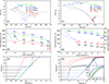 |
Fig. 1. Left: (a1) Evolutionary tracks of four different scenarios of high-mass stars on the HR diagram. A1 and A4 are single-star models (M = 4.5 and M = 3.0 M⊙), and A2 and A3 are mass-accreting and mass-donating models (M = 3.0 → 4.5 M⊙ and M = 4.5 → 3.0 M⊙). (a2) Asymptotic period spacing, ΔP, as a function of the central hydrogen mass fraction, Xc. (a3) Profiles of hydrogen mass fraction, X, for selected models, labelled by different symbols and colours in the corresponding upper and middle panels. Right: (b1) Evolutionary tracks of four different scenarios of low-mass stars on the HR diagram. (b2) Asymptotic period spacing, ΔP, as a function of Xc. (b3) Profiles of hydrogen mass fraction X in the stellar interior for selected models, labelled by different symbols and colours in b1 and b2. |
High-mass case (B stars): Stars evolve with initial masses of Minit = 3 and 4.5 M⊙. As is shown in Figure 1a1, A1 and A4 are the reference evolutionary tracks (no mass transfer, single-star), with initial masses of 4.5 and 3.0 M⊙, respectively.
A2 is a mass-accreting track (3.0 M⊙ → 4.5 M⊙) with an initial mass of Minit = 3.0 M⊙, which begins mass accretion at Xc = 0.45 with a mass-transfer rate of Ṁ = +6 × 10⁻⁸ M⊙/yr. The mass accretion stops at MF = 4.5 M⊙.
A3 is a mass-donating track (4.5 M⊙ → 3.0 M⊙) with an initial mass of Minit = 4.5 M⊙, and the model starts to lose mass at Xc = 0.45 with a rate of Ṁ = −6 × 10⁻⁸ M⊙/yr. The mass donation ends at MF = 3.0 M⊙.
Low-mass case (A, F, G-stars): The initial masses are Minit = 1, and 2 M⊙. Mass transfer is also initiated at Xc = 0.45. The mass transfer rates were set to 3 × 10⁻⁸ M⊙/yr.
As is shown in Figure 1b1, B1 and B4 are the reference evolutionary tracks (no mass transfer), with 2.0 and 1.0 M⊙, respectively.
B2 is a mass-accreting track (1.0 M⊙ → 2.0 M⊙) with a lower initial mass of 1.0 M⊙, which starts to accrete mass at Xc = 0.45 with the mass-accretion rate of Ṁ = +3 × 10⁻⁸ M⊙/yr. Mass accretion ceases at MF = 2.0 M⊙.
B3 is a mass-donating track (2.0 M⊙ → 1.0 M⊙) with an initial mass of 2.0 M⊙, which begins to lose mass at Xc = 0.45 with the mass-change rate of Ṁ = −3 × 10⁻⁸ M⊙/yr. The mass transfer continues until the stellar mass reaches MF = 1.0 M⊙.
Note that the adopted mass-transfer rate (of order 10−8 M⊙/yr for either mass gain or loss) is consistent with a stable RLOF rate for binaries with our adopted stellar masses, as it remains below the accretor’s thermal (Kelvin–Helmholtz, KH) timescale mass-transfer limit, M/tKH (Hurley et al. 2002; Schürmann & Langer 2024).
The evolutionary tracks are shown in the upper panels, a1 and b1, of Figure 1. The asymptotic gravity-mode period spacings (ΔPl = 1) are plotted as functions of the central hydrogen mass fraction, Xc, in panels a2 and b2. Note that for M = 1.0 M⊙ (B4) and M = 2.0 → 1.0 M⊙ (B3) models, the pressure-mode large frequency separation, Δν, is plotted instead of the gravity-mode period spacings (ΔPl = 1) (panel b2). The bottom panels, a3 and b3, display the profiles of hydrogen for selected models, labelled by different symbols and colours in the corresponding upper and middle panels.
These selected models (#-1, #-2, #-3,#-4, #-5) correspond to the central hydrogen, Xc, of 0.4, 0.3, 0.2, 0.1, and 0.01, respectively, where # can be A1 to A4 or B1 to B4. For all panels in Figure 1, green and red denote higher- and lower-mass reference models (and/or tracks), and blue and black represent the models (and/or tracks) with mass donation and mass accretion, respectively.
For single-star models and their tracks (A1 and A4), Figure 1a2 shows that the asymptotic period spacing, ΔΠl = 1 ≈ ΔPl = 1, is slowly decreasing as a function of central hydrogen, Xc. And more massive stars have larger ΔPl = 1 values. We can clearly see the mass-donation effect in A3 (M = 4.5 → 3.0, black curve) from the corresponding decreasing ΔP values (7000 s → 5400 s). Similarly, the mass accretion increases the ΔPl = 1 values (5200 s → 7600 s) for the accretor model (M = 3.0 → 4.5 in blue).
The asymptotic period spacing values, ΔΠl = 1, between model A2-# and A1-#, and between A3-# and A4-#, are of the order of 100 seconds, which is much larger than the typical period resolution of Kepler. This difference can be discerned observationally if accurate stellar stellar masses and ages are known.
3. Asteroseismic imprints of mass accretion and donation
Mass accretion or donation can significantly alter a star’s internal state by changing the temperature, density, and pressure at its core (Kippenhahn & Weigert 1990; Pols 1994; Neo et al. 1977; Renzo & Götberg 2021). For main-sequence stars, these changes can result in a significant fluctuation in the central thermonuclear reaction rate, which in turn impacts the temperature gradient and convective instability (Ledoux 1947; Schwarzschild 1958). This is especially true for the size of the central convective core and the configuration of the chemical (μ) gradient region (as is shown in the bottom panels of Figure 1). Wagg et al. (2024) and Miszuda et al. (2025) show that mass accretion can increase the central temperatures gradient and facilitate the convective core growth (also refer to the bottom panels of Figure 1). This is why the period spacings increase sharply when accreting mass, as is shown by the blue lines in the middle panels of Figure 1.
These mass-transfer-induced changes can persist for an extended period until the region of thermonuclear reactions at the centre moves outwards into the shell beyond the central helium core and the hydrogen shell at the outer region of the μ gradient, which is left by the early central thermonuclear reactions or mass transfer, has been consumed and disrupts the previous state (Paczyński 1971). According to the theory of stellar evolution, the bottom panels of Figure 1 show that, in our calculated cases, the μ gradient imprinting in high-mass scenarios (4.0, 3.0, and 2.0 M⊙) can persist until the stars enter the horizontal branch phase. In comparison, for the low-mass case (M = 1.0 M⊙), stars will lose the signature of the μ gradient during the late stages of the red giant branch (RGB) phase. This means that this signal is preserved throughout most of the star’s lifetime. The induced asteroseismic changes will generally be preserved for a long time and can be detected in observations. It is evident that the formation and persistence of the μ gradient are governed by the characteristics of the mass-transfer process, such as its onset time, rate, and duration.
In this section, we show the asteroseismic imprints of mass accretion and donation by comparing models formed from mass transfer and models formed from single star evolution. We focus on g modes in upper main-sequence stars (M = 3.0, 4.5, and 2.0 M⊙) and p modes in low-mass solar-like stars (M = 1.0 M⊙).
3.1. High-mass scenario
3.1.1. Mass accretion scenario: 3.0 M⊙ → 4.5 M⊙
In Figure 2, we compare two sets of models with the same mass (M = 4.5 M⊙) but different formation histories: one formed from single-star evolution (red), the other from mass accretion (black). For an upper main-sequence star, as is shown in Figure 1 (the red and green lines of panels a3), due to the shrinkage of the central convective core and the burning of the central hydrogen, a gentle μ gradient structure is formed beyond the convective core along with stellar evolution. Rapid mass accretion on the stellar surface will lead to the central temperature, density, and pressure rapidly increasing. The corresponding thermonuclear reaction rate and the corresponding region will be enlarged. This leads to a steeper radiative temperature gradient, which makes the region satisfying the convective instability criterion larger. Thus, the central convective-core boundary will expand and enter the previous receding core during the evolution. The μ gradient structure will be partially or fully removed and a steep or almost discontinuous μ gradient structure (shown in panel a3, blue lines) is formed.
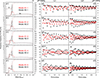 |
Fig. 2. Stellar structure and oscillations of a 4.5 M⊙ star from the single-star model (red) and the mass-accretion model (black). Left panels: Profiles of the buoyancy frequency, N (solid lines: left y axis), and the hydrogen mass fraction, X (dashed lines: right y axis). From top to bottom, the central hydrogen, Xc, values are 0.4, 0.3, 0.2, 0.1, and 0.01. Right panels: Corresponding period spacing patterns of l = 1 and l = 2 g modes. |
When mass accretion stops, stars return to normal evolution in a thermal time scale, and reform a new gently μ gradient structure. Therefore, compared to the normal evolution models, the rapid mass accretion model has narrow μ gradient regions and a steep substructure near the outer edge of the μ gradient areas, which leads to a larger buoyancy frequency, N, as is shown in panels a1–e1 of Figure 2 in this narrow region.
The asymptotic period spacing of g modes, ΔΠl, which is roughly the average level of observed period spacings, ΔP, is defined as
 (1)
(1)
where Λ0 is buoyancy radius and defined as
 (2)
(2)
which is merely related with stellar structure (with the unit of frequency, for instance, Microhertz, i.e., μHz); l is the spherical degree; N is the buoyancy frequency; and r is the radius co-ordinate. As is shown in panel a2 of Figure 1, the period spacings, ΔPl = 1, of the rapid mass accretion models (blue line) are larger than the single-star counterparts (green line) at the same evolutionary states. This is because rapid mass accretion models have slight lower radius (as is shown in panel a1 of Figure 1) and a narrower μ gradient region (as is shown in panels a1–e1 of Figure 2 and panel a3 of Figure 1). Compared with the larger radius and wider μ gradient region of the normal evolution models, the effect of period spacing, ΔP, from the higher buoyancy frequency N value in such a narrow shell can be ignored (as is shown in panels a1–e1 of Figure 2) in rapid mass accretion models.
Similar to Equation (2) and the definition of the acoustic depth of p-mode, the buoyancy depth is defined as (for detailed information refer to e.g. Miglio et al. 2008; Wu et al. 2018, 2020; Wu & Li 2019)
 (3)
(3)
where R is the stellar radius. Similarly, we also define the buoyancy width of the μ gradient region:
 (4)
(4)
where, r1 (r2) is the inner (outer) boundary of the μ gradient region. For a normal intermediate- or massive single main-sequence star model, r1 is the boundary of the centre convective core.
It can be seen from Figure 2 that the average values, varying frequency, and varying amplitude of the period spacing patterns are affected. Comparing the ΔP series in the middle and right panels, we can see that the red (single star) models always have a higher varying frequency and a larger varying amplitude than the black (mass-accretion) models. This is true for all evolutionary stages, from the top to the bottom.
According to the analyses of Wu et al. (2018, refer to their Equation (12) and Figure 5), the higher varying frequency can be explained by the different width of the μ gradient region in buoyancy width, Λμ: wider buoyancy width, higher varying frequency, younger star. The larger period spacing varying amplitude is caused by the higher buoyancy frequency near the outer boundary of μ gradient region and by the narrower buoyancy width, Λμ (more details refer to the Equation (2) of Wu et al. 2020). The larger period spacing varying amplitude of the mass accreting model also would mislead us into regarding the star with fast mass accretion as a younger star than the normal single star. Therefore, the shape of the period spacings varying with period shows that the mass accreting models seem to like younger stars.
The higher varying frequency can also be explained by the μ gradient transition point being at a larger radius (or normalized buoyancy radius, u, see below). The hydrogen mass fraction X profile transition points in the left panels align with the right (outer) edge of the Brunt bump. This right edge is at much larger radius in the red models than in the black models.
The Brunt profiles in the black models also have a spike near the outer edge of the Brunt bump, which is due to the steep μ gradient. The corresponding red models do not have this spike. As is shown by Guo (2025), the Fourier amplitude spectra of period spacings is approximately equal to the buoyancy glitch derivative:
 (5)
(5)
where u is the normalized buoyancy radius defined by
 (6)
(6)
The strong spike in accreting models acts as a large-amplitude buoyancy glitch, which causes g-mode period spacing variation amplitudes to be larger than the red models (middle and right panels).
Another observation is that for models of #-4 and #-5: A1-4 (A2-4) and A1-5 (A2-5), there is a beating pattern in the period spacing series. This is due to the fact that the sampling of ΔP in units of radial order is always 1, and if the ΔP variation frequency is close to 0.5, an interference pattern will arise. This is similar to the Moiré pattern, seen when you take a picture of a computer screen with the cell phone camera: the two arrays of pixels interfere and cause a beating pattern.
The right-hand side of Equation (5) is l-independent. This implies that the ΔP variation frequency or period is the same for l = 1 and l = 2 g modes, counting in the units of radial orders. This is indeed the case in all our calculations (e.g. Figures 2, 3, and 5).
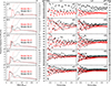 |
Fig. 3. Stellar structure and oscillations of a 3.0 M⊙ star from the single-star model (red) and a mass-donor model (black). Left panels: Profiles of the buoyancy frequency, N (solid lines: left y axis), and the hydrogen mass fraction, X (dashed lines: right y axis). Right panels: Corresponding period spacing patterns of l = 1 and l = 2 g modes. |
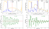 |
Fig. 4. Upper panels: Brunt–Väisälä (buoyancy) frequency profiles (orange) in two accretor models, A3-1 (left) and A3-3 (right). The right panel (i.e., model A3-3) corresponds to the one with additional Brunt bumps. The normalized Fourier spectra of the period spacings of l = 1 g modes is shown as the blue and grey lines (super Nyquist part). The vertical dashed red lines indicate the locations of the Nyquist frequency (0.5). The real peaks corresponding to the period-spacing variation are labelled by the orange squares. Note that in the Fourier spectra of A3-3 model, the dominant peak at 0.53 is above the Nyquist frequency, and its reflection at 0.47 is a fictitious peak. Lower panels: Corresponding period spacings of l = 1 g modes as a function of radial order. |
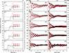 |
Fig. 5. Stellar structure and oscillations of a 2.0 M⊙ star from the single-star model (red) and a mass-accretor model (black). Left panels: Profiles of the buoyancy frequency, N (solid lines: left y axis) and the hydrogen mass fraction X (dashed lines: right y axis). Right panels: Corresponding period spacing patterns of l = 1 and l = 2 g modes. |
3.1.2. Mass donation case: 4.5 M⊙ → 3.0 M⊙
In Figure 3, we compare two sets of models with the same mass (M = 3.0 M⊙) but different formation histories: one from single-star evolution (red), the other from mass donation (black). As is shown in the middle and right panels, the most prominent difference is the additional periodicities in the ΔP series for the black models (donor) compared to the red models (single star). This is due to the retreat of the convective core when the mass donation occurs at Xc = 0.45 (between panel a1 and panel b1 in the left panel), which produces an additional chemical composition transition zone (two pronounced nested depletion zones, characterized by two broad troughs in the X profile), and thus an additional Brunt bump at around 0.5 in mass co-ordinate. Two Brunt bumps are present in the A3-2, A3-3, A3-4, and A3-5 models, while the corresponding single-star models in red (A4-2, A4-3, A3-4, and A4-5) have only one Brunt bump.
To quantify the periodicity in the ΔP series, we performed the Fourier transform of the ΔP with respect to the radial order, n, and show the results in Figure 4. As can be seen, the right-edge of Brunt bump aligns with the dominant peak in the Fourier spectra of ΔP series. For A3-1, only one dominant peak at u ∼ 0.25 is present, corresponding to a mono-periodic variation in ΔP. This is the case for both A3-1 and A4-1, although A4-1 period spacings have much lower mean values (ΔΠl). The real peak at u = 0.25 labelled by the orange square is reflected to 0.75 in the super-Nyquist (grey) part.
Starting from A3-2, two dominant peaks are present in the Fourier spectra due to the two right edges (sharp dropping) of the two Brunt bumps. As can be seen in the right panel of Figure 4, the A3-3 model g-mode period spacings have two variation frequencies, at ∼0.2 and ∼0.48. The grey part of the Fourier spectra is super Nyquist, and is a mirror of the sub-Nyquist (< 0.5) part. For mode A3-3, the real peaks are at ∼0.16 and 0.53, marked by the orange squares. These two real frequencies are reflected around 0.5 and produce two fictitious peaks at 0.84 and 0.47. Note that the left edge of the Brunt bump also contributes to another frequency (∼0.35) in the ΔP variation, but at a smaller amplitude. It is worth noting that the width between the two μ gradient regions is fully determined by the duration of the mass-loss phase and the mass loss rate. Also note the higher mean levels of the ΔP series for the black models than the red models, due to the integration of N/r (Equation (1)) in the mode propagation cavity is larger for the red models, resulting in a lower asymptotic period spacing ΔΠl (also see the black line in panel a2 of Figure 2).
3.2. Low-mass scenario
3.2.1. Mass accretion case: 1.0 M⊙ → 2.0 M⊙
Figure 5 illustrates how two stars of the same mass (2.0 M⊙) can differ structurally depending on their formation channel: single-star evolution (red) versus mass accretion (black). The left panels illustrate how the Brunt-Väisälä frequency (N) and hydrogen mass fraction (X) vary within the stellar interior in the mass co-ordinates. Note that the X profiles of the two models (dotted red and black lines) are nearly identical, almost overlapping. This is already shown in Figure 1, panel b3, where the blue and green lines also almost coincide. The Brunt profiles are also very similar, with the red model having a slightly wider Brunt bump and a small-amplitude kink close to the right-edge of the bump. This is similar to the additional Brunt kink in the M = 3.5 M⊙ accretor model calculated by Wagg et al. (2024) (their Figure 4).
Since the right-edge of Brunt bump is at a larger radial or mass co-ordinate (a larger buoyancy radius). This suggests a slightly higher frequency in the ΔP variation for red models. There is also a small phase shift between the red and black ΔP series due to the difference in the Brunt profile. Other than these two differences, the ΔP series are very similar, they largely have the similar variation frequency and amplitude, and mean levels.
This means that it is very difficult to clearly distinguish the normal single star and the mass accretion model from their period spacing shapes for such a low-mass case directly. Detailed modelling is necessary for making informed decisions.
3.2.2. Mass donation case: 2.0 M⊙ → 1.0 M⊙
It is evident that our previous analysis centred on g-mode pulsations, which are characteristic of SPB and γ Dor pulsating variable stars. In this next phase of our analysis, we shift our focus to p-mode pulsations, specifically solar-like oscillations. This transition is motivated by the presence of substantial outer convective envelopes in these stars, which inhibit g modes from reaching the stellar surface, and thus from being observed. In these cases, the pulsations are excited stochastically by convective turbulence, similar to the processes operating in the Sun.
Figure 6 contrasts two models of identical mass (1.0 M⊙) that follow distinct evolutionary paths – one formed through single-star evolution (red) and the other through mass donation (black). The left panels show the Lamb frequency profile,  (in logarithm), and hydrogen mass fraction, X, as functions of the enclosed mass, where cs is adiabatic sound speed and kh is the horizontal wave number of acoustic waves. We can immediately see the vastly different X profiles for the red (single star) and black (mass-donor) models. This is also shown in panel b3 of Figure 1 (red and black lines, respectively). Although the two stellar models have the same mass and radius, the donor model still pertains the convective core from the initial mass of M = 2.0 M⊙ model. The hydrogen profiles, X(m), exhibit a distinct depletion region near the stellar core, forming a broad trough just outside the convective core boundary. In the more evolved models, it develops two nested depressions, reflecting successive chemical-composition gradients produced by core contraction after mass transfer. The additional ‘trough’ is due to the mass donation. This is similar to the high-mass donor models case (M = 3.0 M⊙, see Figure 3). In contrast, the single-star (1.0 M⊙) model, equivalent to the Sun, has a radiative core and a smooth X profile (dashed red lines in Figure 6 left panel; red lines in Figure 1b3).
The middle panels of Figure 6 show the p-mode frequency separation ratios between small and large frequency separations: r01, r10 (squares and triangles), and r02 (circles). These frequency ratios are defined as follows (Buldgen et al. 2022):
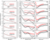 |
Fig. 6. Stellar structure and oscillations of a 1.0 M⊙ star from the single-star model (red) and a mass-donor model (black). Left panels: Profiles of the Lamb frequency, log Sl = 1 (solid lines: left y axis), and the hydrogen mass fraction, X (dashed lines: right y axis), in the mass co-ordinates (x axis). Middle panels: Corresponding acoustic-model frequency separation ratios, r01, r10, and r02 (squares, triangles, and circles), between small and large frequency separations, respectively, which are calculated with Equations (7). Right panels: Normalized large-frequency separation (Δνl/⟨Δνl⟩) (l = 0, 1, 2, corresponding to squares, triangles, and circles) as a function of radial order (n). |
 (7)
(7)
The large frequency separation as a function of the radial order is Δνl(n) = νn, l − νn − 1, l. The small frequency separation is δ02(n) = νn, 0 − νn − 1, 2. The definitions of middle-point small separations, δ01 and δ10, are expressed as
 (8)
(8)
It is well known that the small separations are sensitive to the sound-speed gradient in the stellar core (Christensen-Dalsgaard 1984; Roxburgh & Vorontsov 2003; Roxburgh 2009).
In Figure 6, the gradient of the Lamb frequency exhibits discontinuities (sign changes) at locations where the hydrogen abundance, X, varies sharply in the mass-donor model (black). These features are most prominent at mass co-ordinates of approximately 0.1 and 0.35 − 0.4, where the slope of log Sl in the left panels changes from negative (decreasing) to positive (increasing) values. These features can act as acoustic glitches and cause periodic variations in the small frequency separations. The variation amplitude depends on the gradient of acoustic glitch with respect to acoustic co-ordinate d(δc/c)/dlnΦ (Guo, in prep.), and the variation frequency (reciprocal of cycles measured in units of the radial order) is just the local relative acoustic radius, Φ(rglitch), of the glitch (Roxburgh & Vorontsov 1994; Montgomery et al. 2003; Miglio et al. 2010). Φ(r) is defined as
 (9)
(9)
where r1 is the inner boundary, R is the outer boundary of the acoustic wave. As can be seen in the left panels, the red model has a smoother X profile, and thus a smoother sound-speed (Lamb frequency) gradient. The small separation ratios do not show periodic variations (red curve in middle panels). This is the reason for the vastly different small separation ratios (smooth red curves vs oscillatory black curves) in the middle panels. However, the global large frequency separations, Δν (right panels), are more similar for both models. This is because the variation in Δν with radial order n is primarily sensitive to the stellar envelope structure, rather than the core structure that differentiates the two models.
In summary, the above analyses show that the asteroseismic signals caused by mass accretion are probably too weak to be directly identified from the shape of the period-spacing series, regardless of whether it is a high-mass or low-mass scenario. Detailed asteroseismic modelling might be an effective approach to distinguish mass-accretion stars from normal single stars. In contrast, for mass-donation (loss) scenarios in both high-mass and low-mass cases, the additional asteroseismic signals are prominent and they could be directly recognized from their period-spacing series or frequency-separation ratios.
4. Discussion and conclusion
Mass accretor and donor models exhibit internal structures that are markedly different from those of single-star counterparts. The main-sequence evolution of intermediate- and high-mass stars naturally produces a hydrogen abundance gradient outside the convective core, which leaves a distinct chemical transition zone. In a binary system, this process can be interrupted by mass transfer. When mass is accreted onto a star, the central pressure and temperature increase, the nuclear energy generation rate rises, and the convective core expands. Conversely, in a donor undergoing mass loss, the opposite occurs: the core retreats, and the chemical gradient steepens. These contrasting responses produce pronounced structural and asteroseismic differences between accretors, donors, and single-star models.
The sharp chemical composition transition zones (additional spikes or troughs) in the X profiles induce additional kinks or broad bumps in the Brunt profile. The corresponding g-mode period spacing series show additional periodic modulations, whose amplitude depends on the gradient of the Brunt glitch and whose frequency depends on the location of the buoyancy glitch. Fourier spectrum of g-mode period spacings are particularly useful because the dominant peaks’ locations and amplitudes are just the ΔP variation frequency and glitch gradient amplitude, respectively. This explains the g-mode period spacing differences in our M = 3.0, 4.5, 2.0 M⊙ models.
For solar-type models, we find that a mass-donation episode can fundamentally alter the internal structure: a donor remnant near 1 M⊙ can retain a small convective core, unlike a normal solar-mass star with a radiative core. Moreover, the sound speed gradient profile can display multiple discontinuities, each acting as a potential acoustic glitch. These features modulate p-mode frequency separations and ratios in a measurably way. Such behaviour, if confirmed observationally, would open a new window into the internal structure of post–mass-transfer solar-like oscillators.
Our results demonstrate that the asteroseismic signatures of mass exchange are, in principle, observable. The characteristic double or multiple periodicities in the g-mode period spacings serve as ‘seismic fossils’ of a star’s binary-interaction history. Detecting these signatures requires a sufficient number of consecutive g modes, which is now achievable thanks to continuous high-precision photometry from TESS (Ricker et al. 2015) and will be further enhanced by PLATO (Rauer et al. 2025) and ET (Ge et al. 2022, 2024a,b). A systematic search for post–mass-transfer pulsators, combining photometric variability, binary light curves, and spectroscopic characterization, could yield the first observational constraints on historical mass-transfer rates and timings in binary systems.
The implications extend beyond individual stars. Binary mass exchange is common among intermediate- and massive-star populations. In this sense, asteroseismology provides a complementary tool to discover interior evidence for rejuvenation or stripping events.
We summarize the main limitations of the present work.
(1) We have assumed that the accreted material has the same composition as the accretor’s surface. In reality, the transferred material may be helium-enriched or CNO-processed, leading to density inversions and thermohaline (double-diffusive) instabilities (Ulrich 1972; Stancliffe & Glebbeek 2008). These processes act on a KH timescale,  . The interplay between such mixing and mode excitations remains to be quantified. Extending the current adiabatic stellar oscillation calculations to include non-adiabatic effects would provide valuable insights.
(2) We ignore the important effect of rotation on stellar oscillations. Apart from shifting the oscillation frequencies, it is also known that the fast rotation suppresses the p-mode amplitudes in δ Scuti stars and affects the mode stability of g modes and r modes in γ Dor and SPB stars. Mass accretion naturally leads to fast rotating accretors, both the rotation and temperature affects the g modes of the accretor significantly. A similar study of the accretion effect on stellar oscillations such as Arras et al. (2006) and Kumar & Townsley (2023) but for other pulsators is desirable.
(3) We use a fixed mass gain and loss rate, while in a real binary system, the mass transfer rate is determined by the orbital configuration and mass ratios (Kolb & Ritter 1990). We could perform a detailed binary star evolution with the MESA-binary. It is interesting to explore different mass-transfer rates and their effect on the stellar oscillations of the post-mass-transfer stars. The stability of mass transfer plays a crucial role in determining the final evolutionary outcomes (Soberman et al. 1997) and the likelihood of detecting oscillations in the resulting systems.
(4) From Equation (5), we can see the variation amplitude and frequency in the ΔP is spherical degree l independent. But more information can be extracted from the mode phases. The l = 1 and l = 2 g modes have slightly different mode propagation cavities and turning points.
(5) Other post-mass-transfer pulsators and binary populations. In this work, we focus exclusively on the effects of mass transfer on upper–main-sequence pulsators. As was outlined in the introduction, a wide variety of post–mass-transfer pulsators populate different regions of the Hertzsprung–Russell diagram. A comprehensive ‘pulsator HR’ diagram for binary systems – similar to that presented by Kurtz (2022) and population synthesis such as Hurley et al. (2002) – would be highly valuable. Dedicated modelling efforts are required for each class of post–mass-transfer pulsators, and such studies are already emerging, for example in recent work on blue stragglers (Briganti et al. 2025).
Next, we shall use a binary star evolution code to simulate the actual evolution of a binary system, including the processes of mass transfer, stellar rotation, and orbital evolution, while taking into account the simultaneous evolution of both stars. Most of the above deficiencies will be effectively addressed.
Acknowledgments
This work is co-supported by the National Natural Science Foundation of China (Grant No. 12288102), the B-type Strategic Priority Program of the Chinese Academy of Sciences (Grant No. XDB1160202), and the National Key R&D Program of China (Grant No. 2021YFA1600400/2021YFA1600402). ZG thanks to the funding from the European Research Council (ERC) under the Horizon Europe programme (Synergy Grant agreement No. 101071505: 4D-STAR). While funded by the European Union, views and opinions expressed are however those of the author(s) only and do not necessarily reflect those of the European Union or the European Research Council. Neither the European Union nor the granting authority can be held responsible for them. ZG is also supported by STFC grant UKRI1179. TW and YL also gratefully acknowledge the supports of NSFC of China (Grant Nos. 11973079, 12133011 and 12273104), Yunnan Fundamental Research Projects (Grant No. 202401AS070045), Youth Innovation Promotion Association of Chinese Academy of Sciences, Ten Thousand Talents Program of Yunnan for Top-notch Young Talents, the International Centre of Supernovae, Yunnan Key Laboratory (No. 202302AN360001), and China Manned Space Program (Grant No. CMS-CSST-2025-A14/A01). The authors gratefully acknowledge the computing time granted by the Yunnan Observatories, and provided on the facilities at the Yunnan Observatories Supercomputing Platform and the “PHOENIX Supercomputing Platform” jointly operated by the Binary Population Synthesis Group and The Stellar Astrophysics Group at Yunnan Observatories, Chinese Academy of Sciences. And finally, the authors are cordially grateful to an anonymous referee for instructive advice and productive suggestions that significantly improved the quality of this paper.
References
- Aerts, C., Christensen-Dalsgaard, J., & Kurtz, D. W. 2010, Asteroseismology (Springer Science+Business Media B.V.) [Google Scholar]
- Arras, P., Townsley, D. M., & Bildsten, L. 2006, ApJ, 643, L119 [Google Scholar]
- Basu, S., & Chaplin, W. J. 2017, Asteroseismic Data Analysis: Foundations and Techniques (Princeton University Press) [Google Scholar]
- Belczynski, K., Kalogera, V., & Bulik, T. 2002, ApJ, 572, 407 [NASA ADS] [CrossRef] [Google Scholar]
- Bondi, H., & Hoyle, F. 1944, MNRAS, 104, 273 [Google Scholar]
- Briganti, L., van Rossem, W. E., Miglio, A., Bragaglia, A., & Matteuzzi, M. 2025, A&A, 704, L15 [NASA ADS] [CrossRef] [EDP Sciences] [Google Scholar]
- Buldgen, G., Bétrisey, J., Roxburgh, I. W., Vorontsov, S. V., & Reese, D. R. 2022, Front. Astron. Space Sci., 9, 942373 [NASA ADS] [CrossRef] [Google Scholar]
- Cehula, J., & Pejcha, O. 2023, MNRAS, 524, 471 [NASA ADS] [CrossRef] [Google Scholar]
- Chen, X., & Han, Z. 2009, MNRAS, 395, 1822 [Google Scholar]
- Chen, X., Maxted, P. F. L., Li, J., & Han, Z. 2017, MNRAS, 467, 1874 [NASA ADS] [CrossRef] [Google Scholar]
- Christensen-Dalsgaard, J. 1984, in Space Research in Stellar Activity and Variability, eds. A. Mangeney, & F. Praderie, 11 [Google Scholar]
- Córsico, A. H., Althaus, L. G., Miller Bertolami, M. M., & Kepler, S. O. 2019, A&ARv, 27, 7 [Google Scholar]
- Cox, J. P., & Giuli, R. T. 1968, Principles of Stellar Structure (New York: Gordon and Breach) [Google Scholar]
- de Mink, S. E., Langer, N., Izzard, R. G., Sana, H., & de Koter, A. 2013, ApJ, 764, 166 [Google Scholar]
- Deheuvels, S., Ballot, J., Gehan, C., & Mosser, B. 2022, A&A, 659, A106 [NASA ADS] [CrossRef] [EDP Sciences] [Google Scholar]
- Eggleton, P. P. 1983, ApJ, 268, 368 [Google Scholar]
- Farrell, E., Buldgen, G., Meynet, G., et al. 2024, A&A, 686, A267 [NASA ADS] [CrossRef] [EDP Sciences] [Google Scholar]
- Gautschy, A., & Saio, H. 2017, MNRAS, 468, 4419 [NASA ADS] [CrossRef] [Google Scholar]
- Ge, H., Webbink, R. F., Chen, X., & Han, Z. 2015, ApJ, 812, 40 [Google Scholar]
- Ge, J., Zhang, H., Zang, W., et al. 2022, ArXiv e-prints [arXiv:2206.06693] [Google Scholar]
- Ge, J., Chen, W., Chen, Y., et al. 2024a, Chin. J. Space Sci., 44, 400 [Google Scholar]
- Ge, J., Zhang, H., Zhang, Y., et al. 2024b, SPIE Conf. Ser., 13092, 1309218 [Google Scholar]
- Gianninas, A., Curd, B., Fontaine, G., Brown, W. R., & Kilic, M. 2016, ApJ, 822, L27 [Google Scholar]
- Gies, D. R., Guo, Z., Howell, S. B., et al. 2013, ApJ, 775, 64 [Google Scholar]
- Grevesse, N., & Sauval, A. J. 1998, Space Sci. Rev., 85, 161 [Google Scholar]
- Guo, Z. 2021, Front. Astron. Space Sci., 8, 67 [NASA ADS] [Google Scholar]
- Guo, Z. 2025, A&A, submitted [arXiv:2511.05780] [Google Scholar]
- Guo, Z., Gies, D. R., Matson, R. A., et al. 2017a, ApJ, 837, 114 [NASA ADS] [CrossRef] [Google Scholar]
- Guo, Z., Gies, D. R., & Matson, R. A. 2017b, ApJ, 851, 39 [NASA ADS] [CrossRef] [Google Scholar]
- Han, Z., Podsiadlowski, P., & Eggleton, P. P. 1995, MNRAS, 272, 800 [NASA ADS] [Google Scholar]
- Han, Z., Podsiadlowski, P., Maxted, P. F. L., Marsh, T. R., & Ivanova, N. 2002, MNRAS, 336, 449 [Google Scholar]
- Hatta, Y. 2023, ApJ, 950, 165 [NASA ADS] [CrossRef] [Google Scholar]
- Henneco, J., Schneider, F. R. N., Hekker, S., & Aerts, C. 2024, A&A, 690, A65 [NASA ADS] [CrossRef] [EDP Sciences] [Google Scholar]
- Henneco, J., Schneider, F. R. N., Heller, M., Hekker, S., & Aerts, C. 2025, A&A, 698, A49 [NASA ADS] [CrossRef] [EDP Sciences] [Google Scholar]
- Herwig, F. 2000, A&A, 360, 952 [NASA ADS] [Google Scholar]
- Hurley, J. R., Tout, C. A., & Pols, O. R. 2002, MNRAS, 329, 897 [Google Scholar]
- Iben, I., & Livio, M. 1993, PASP, 105, 1373 [CrossRef] [Google Scholar]
- Iglesias, C. A., & Rogers, F. J. 1996, ApJ, 464, 943 [NASA ADS] [CrossRef] [Google Scholar]
- Istrate, A. G., Fontaine, G., Gianninas, A., et al. 2016a, A&A, 595, L12 [NASA ADS] [CrossRef] [EDP Sciences] [Google Scholar]
- Istrate, A. G., Marchant, P., Tauris, T. M., et al. 2016b, A&A, 595, A35 [NASA ADS] [CrossRef] [EDP Sciences] [Google Scholar]
- Karczmarek, P., Wiktorowicz, G., Iłkiewicz, K., et al. 2017, MNRAS, 466, 2842 [CrossRef] [Google Scholar]
- Kippenhahn, R., & Weigert, A. 1967, ZAp, 65, 251 [Google Scholar]
- Kippenhahn, R., & Weigert, A. 1990, Stellar Structure and Evolution (New York: Springer-Verlag) [Google Scholar]
- Kolb, U., & Ritter, H. 1990, A&A, 236, 385 [NASA ADS] [Google Scholar]
- Kopal, Z. 1959, Close Binary Systems (London: Chapman& Hall) [Google Scholar]
- Kumar, P., & Townsley, D. M. 2023, ApJ, 951, 122 [Google Scholar]
- Kurtz, D. W. 2022, ARA&A, 60, 31 [NASA ADS] [CrossRef] [Google Scholar]
- Langer, N. 2012, ARA&A, 50, 107 [CrossRef] [Google Scholar]
- Laplace, E., Götberg, Y., de Mink, S. E., Justham, S., & Farmer, R. 2020, A&A, 637, A6 [NASA ADS] [CrossRef] [EDP Sciences] [Google Scholar]
- Lauterborn, D. 1970, A&A, 7, 150 [NASA ADS] [Google Scholar]
- Ledoux, P. 1947, ApJ, 105, 305 [NASA ADS] [CrossRef] [Google Scholar]
- Li, Y., Bedding, T. R., Murphy, S. J., et al. 2022, Nat. Astron., 6, 673 [NASA ADS] [CrossRef] [Google Scholar]
- Li, G., Deheuvels, S., & Ballot, J. 2024, A&A, 688, A184 [NASA ADS] [CrossRef] [EDP Sciences] [Google Scholar]
- Maxted, P. F. L., Serenelli, A. M., Miglio, A., et al. 2013, Nature, 498, 463 [Google Scholar]
- Miglio, A., Montalbán, J., Noels, A., & Eggenberger, P. 2008, MNRAS, 386, 1487 [Google Scholar]
- Miglio, A., Montalbán, J., Carrier, F., et al. 2010, A&A, 520, L6 [CrossRef] [EDP Sciences] [Google Scholar]
- Miszuda, A. 2025, A&A, 701, L7 [NASA ADS] [CrossRef] [EDP Sciences] [Google Scholar]
- Miszuda, A., Szewczuk, W., & Daszyńska-Daszkiewicz, J. 2021, MNRAS, 505, 3206 [NASA ADS] [CrossRef] [Google Scholar]
- Miszuda, A., Kołaczek-Szymański, P. A., Szewczuk, W., & Daszyńska-Daszkiewicz, J. 2022, MNRAS, 514, 622 [NASA ADS] [CrossRef] [Google Scholar]
- Miszuda, A., Guo, Z., & Townsend, R. H. D. 2025, A&A, 702, A203 [NASA ADS] [CrossRef] [EDP Sciences] [Google Scholar]
- Mkrtichian, D. E., Kusakin, A. V., Rodriguez, E., et al. 2004, A&A, 419, 1015 [NASA ADS] [CrossRef] [EDP Sciences] [Google Scholar]
- Mkrtichian, D. E., Lehmann, H., Rodríguez, E., et al. 2018, MNRAS, 475, 4745 [NASA ADS] [CrossRef] [Google Scholar]
- Moe, M., & Di Stefano, R. 2017, ApJS, 230, 15 [Google Scholar]
- Montgomery, M. H., Metcalfe, T. S., & Winget, D. E. 2003, MNRAS, 344, 657 [NASA ADS] [CrossRef] [Google Scholar]
- Moravveji, E., Aerts, C., Pápics, P. I., Triana, S. A., & Vandoren, B. 2015, A&A, 580, A27 [NASA ADS] [CrossRef] [EDP Sciences] [Google Scholar]
- Neo, S., Miyaji, S., Nomoto, K., & Sugimoto, D. 1977, PASJ, 29, 249 [NASA ADS] [Google Scholar]
- Packet, W. 1981, A&A, 102, 17 [NASA ADS] [Google Scholar]
- Paczyński, B. 1971, ARA&A, 9, 183 [Google Scholar]
- Paxton, B., Bildsten, L., Dotter, A., et al. 2011, ApJS, 192, 3 [Google Scholar]
- Paxton, B., Cantiello, M., Arras, P., et al. 2013, ApJS, 208, 4 [Google Scholar]
- Paxton, B., Marchant, P., Schwab, J., et al. 2015, ApJS, 220, 15 [Google Scholar]
- Paxton, B., Schwab, J., Bauer, E. B., et al. 2018, ApJS, 234, 34 [NASA ADS] [CrossRef] [Google Scholar]
- Perets, H. B., & Šubr, L. 2012, ApJ, 751, 133 [Google Scholar]
- Pietrzyński, G., Thompson, I. B., Gieren, W., et al. 2012, Nature, 484, 75 [CrossRef] [Google Scholar]
- Pilecki, B., Gieren, W., Smolec, R., et al. 2017, ApJ, 842, 110 [Google Scholar]
- Pols, O. R. 1994, A&A, 290, 119 [Google Scholar]
- Rappaport, S., Verbunt, F., & Joss, P. C. 1983, ApJ, 275, 713 [Google Scholar]
- Rauer, H., Aerts, C., Cabrera, J., et al. 2025, Exp. Astron., 59, 26 [Google Scholar]
- Renzo, M., & Götberg, Y. 2021, ApJ, 923, 277 [NASA ADS] [CrossRef] [Google Scholar]
- Ricker, G. R., Winn, J. N., Vanderspek, R., et al. 2015, J. Astron. Telesc. Instrum. Syst., 1, 014003 [Google Scholar]
- Rivinius, T., Carciofi, A. C., & Martayan, C. 2013, A&ARv, 21, 69 [Google Scholar]
- Roxburgh, I. W. 2009, A&A, 493, 185 [NASA ADS] [CrossRef] [EDP Sciences] [Google Scholar]
- Roxburgh, I. W., & Vorontsov, S. V. 1994, MNRAS, 268, 880 [NASA ADS] [CrossRef] [Google Scholar]
- Roxburgh, I. W., & Vorontsov, S. V. 2003, A&A, 411, 215 [NASA ADS] [CrossRef] [EDP Sciences] [Google Scholar]
- Rui, N. Z., & Fuller, J. 2021, MNRAS, 508, 1618 [NASA ADS] [CrossRef] [Google Scholar]
- Sana, H., de Mink, S. E., de Koter, A., et al. 2012, Science, 337, 444 [Google Scholar]
- Schneider, F. R. N. 2025, ArXiv e-prints [arXiv:2509.18421] [Google Scholar]
- Schürmann, C., & Langer, N. 2024, A&A, 691, A174 [NASA ADS] [CrossRef] [EDP Sciences] [Google Scholar]
- Schwarzschild, M. 1958, Structure and Evolution of Stars (Princeton University Press) [Google Scholar]
- Soberman, G. E., Phinney, E. S., & van den Heuvel, E. P. J. 1997, A&A, 327, 620 [NASA ADS] [Google Scholar]
- Southworth, J., & Bowman, D. 2025, ArXiv e-prints [arXiv:2509.08426] [Google Scholar]
- Stancliffe, R. J., & Glebbeek, E. 2008, MNRAS, 389, 1828 [Google Scholar]
- Streamer, M., Ireland, M. J., Murphy, S. J., & Bento, J. 2018, MNRAS, 480, 1372 [NASA ADS] [CrossRef] [Google Scholar]
- Sun, M., Townsend, R. H. D., & Guo, Z. 2023, ApJ, 945, 43 [NASA ADS] [CrossRef] [Google Scholar]
- Tauris, T. M., & van den Heuvel, E. P. J. 2006, in Compact Stellar X-ray Sources, eds. W. H. G. Lewin, & M. van der Klis, 39, 623 [NASA ADS] [CrossRef] [Google Scholar]
- Tauris, T. M., & van den Heuvel, E. P. J. 2023, Physics of Binary Star Evolution. From Stars to X-ray Binaries and Gravitational Wave Sources (Princeton University Press) [Google Scholar]
- Townsend, R. H. D., & Teitler, S. A. 2013, MNRAS, 435, 3406 [Google Scholar]
- Townsend, R. H. D., Goldstein, J., & Zweibel, E. G. 2018, MNRAS, 475, 879 [Google Scholar]
- Ulrich, R. K. 1972, ApJ, 172, 165 [NASA ADS] [CrossRef] [Google Scholar]
- Vanbeveren, D., De Loore, C., & Van Rensbergen, W. 1998, A&ARv, 9, 63 [Google Scholar]
- Wagg, T., Johnston, C., Bellinger, E. P., et al. 2024, A&A, 687, A222 [NASA ADS] [CrossRef] [EDP Sciences] [Google Scholar]
- Webbink, R. F. 1976, ApJS, 32, 583 [Google Scholar]
- Webbink, R. F. 1984, ApJ, 277, 355 [NASA ADS] [CrossRef] [Google Scholar]
- Willems, B., & Kolb, U. 2004, A&A, 419, 1057 [NASA ADS] [CrossRef] [EDP Sciences] [Google Scholar]
- Wu, T., & Li, Y. 2019, ApJ, 881, 86 [Google Scholar]
- Wu, T., Li, Y., & Deng, Z.-M. 2018, ApJ, 867, 47 [NASA ADS] [CrossRef] [Google Scholar]
- Wu, T., Li, Y., Deng, Z.-M., et al. 2020, ApJ, 899, 38 [NASA ADS] [CrossRef] [Google Scholar]
- Zhang, Q.-S., Li, Y., Wu, T., & Jiang, C. 2023, ApJ, 953, 9 [NASA ADS] [CrossRef] [Google Scholar]
Appendix A: MESA inlists
A.1. Inlist for signal star with mass loss or accretion: inlist_astero_gyre
&star_job

change_initial_net = .true.
new_net_name = 'cno_extras_o18_and_ne22.net'
create_pre_main_sequence_model = .true.
set_initial_cumulative_energy_error = .true.
new_cumulative_energy_error = 0d0

/ ! end of star_job namelist

&controls

initial_mass = 2.d0 !2.002713d0 !1.d0
initial_z = 0.02d0
mass_change = -6d-5
max_star_mass_for_gain = 1.d0
!min_star_mass_for_loss = 2d0
accrete_same_as_surface = .true.!
mixing_length_alpha = 2d0
max_years_for_timestep = 3d6 !8d6 !3d6
mesh_delta_coeff = 0.5  !0.3 ==> 5100
varcontrol_target = 1d-4
mesh_logX_species(1) = 'h1'
mesh_logX_min_for_extra(1) = -4
mesh_dlogX_dlogP_extra(1) = 0.2
mesh_dlogX_dlogP_full_on(1) = 1d-3
mesh_dlogX_dlogP_full_off(1) = 1d-5
calculate_Brunt_N2 = .true.
smooth_convective_bdy = .true.
num_cells_for_smooth_brunt_B = 10
num_cells_for_smooth_gradL_composition_term = 10
set_min_D_mix = .true.
mass_lower_limit_for_min_D_mix = 0d0
mass_upper_limit_for_min_D_mix = 1d99
min_D_mix = 5d-1 !1d1

overshoot_scheme = 'exponential' ! exponential, step
overshoot_zone_type = 'any' ! burn_H,_He,_Z, nonburn, any
overshoot_zone_loc = 'core' !  core, shell, any
overshoot_bdy_loc = 'top'  ! bottom, top, any`

overshoot_f = 0.016d0
overshoot_f0 = 0.001d0
write_pulse_data_with_profile =.TRUE.! .false. !
pulse_data_format = 'GYRE'

/ ! end of controls namelist
All Figures
|
Fig. 1. Left: (a1) Evolutionary tracks of four different scenarios of high-mass stars on the HR diagram. A1 and A4 are single-star models (M = 4.5 and M = 3.0 M⊙), and A2 and A3 are mass-accreting and mass-donating models (M = 3.0 → 4.5 M⊙ and M = 4.5 → 3.0 M⊙). (a2) Asymptotic period spacing, ΔP, as a function of the central hydrogen mass fraction, Xc. (a3) Profiles of hydrogen mass fraction, X, for selected models, labelled by different symbols and colours in the corresponding upper and middle panels. Right: (b1) Evolutionary tracks of four different scenarios of low-mass stars on the HR diagram. (b2) Asymptotic period spacing, ΔP, as a function of Xc. (b3) Profiles of hydrogen mass fraction X in the stellar interior for selected models, labelled by different symbols and colours in b1 and b2. |
| In the text | |
|
Fig. 2. Stellar structure and oscillations of a 4.5 M⊙ star from the single-star model (red) and the mass-accretion model (black). Left panels: Profiles of the buoyancy frequency, N (solid lines: left y axis), and the hydrogen mass fraction, X (dashed lines: right y axis). From top to bottom, the central hydrogen, Xc, values are 0.4, 0.3, 0.2, 0.1, and 0.01. Right panels: Corresponding period spacing patterns of l = 1 and l = 2 g modes. |
| In the text | |
|
Fig. 3. Stellar structure and oscillations of a 3.0 M⊙ star from the single-star model (red) and a mass-donor model (black). Left panels: Profiles of the buoyancy frequency, N (solid lines: left y axis), and the hydrogen mass fraction, X (dashed lines: right y axis). Right panels: Corresponding period spacing patterns of l = 1 and l = 2 g modes. |
| In the text | |
|
Fig. 4. Upper panels: Brunt–Väisälä (buoyancy) frequency profiles (orange) in two accretor models, A3-1 (left) and A3-3 (right). The right panel (i.e., model A3-3) corresponds to the one with additional Brunt bumps. The normalized Fourier spectra of the period spacings of l = 1 g modes is shown as the blue and grey lines (super Nyquist part). The vertical dashed red lines indicate the locations of the Nyquist frequency (0.5). The real peaks corresponding to the period-spacing variation are labelled by the orange squares. Note that in the Fourier spectra of A3-3 model, the dominant peak at 0.53 is above the Nyquist frequency, and its reflection at 0.47 is a fictitious peak. Lower panels: Corresponding period spacings of l = 1 g modes as a function of radial order. |
| In the text | |
|
Fig. 5. Stellar structure and oscillations of a 2.0 M⊙ star from the single-star model (red) and a mass-accretor model (black). Left panels: Profiles of the buoyancy frequency, N (solid lines: left y axis) and the hydrogen mass fraction X (dashed lines: right y axis). Right panels: Corresponding period spacing patterns of l = 1 and l = 2 g modes. |
| In the text | |
|
Fig. 6. Stellar structure and oscillations of a 1.0 M⊙ star from the single-star model (red) and a mass-donor model (black). Left panels: Profiles of the Lamb frequency, log Sl = 1 (solid lines: left y axis), and the hydrogen mass fraction, X (dashed lines: right y axis), in the mass co-ordinates (x axis). Middle panels: Corresponding acoustic-model frequency separation ratios, r01, r10, and r02 (squares, triangles, and circles), between small and large frequency separations, respectively, which are calculated with Equations (7). Right panels: Normalized large-frequency separation (Δνl/⟨Δνl⟩) (l = 0, 1, 2, corresponding to squares, triangles, and circles) as a function of radial order (n). |
| In the text | |
Current usage metrics show cumulative count of Article Views (full-text article views including HTML views, PDF and ePub downloads, according to the available data) and Abstracts Views on Vision4Press platform.
Data correspond to usage on the plateform after 2015. The current usage metrics is available 48-96 hours after online publication and is updated daily on week days.
Initial download of the metrics may take a while.