| Issue |
A&A
Volume 706, February 2026
|
|
|---|---|---|
| Article Number | A312 | |
| Number of page(s) | 17 | |
| Section | Planets, planetary systems, and small bodies | |
| DOI | https://doi.org/10.1051/0004-6361/202449743 | |
| Published online | 23 February 2026 | |
Imaging the LkCa 15 system in polarimetry and total intensity without self-subtraction artefacts★
1
Dipartimento di Fisica, Università degli Studi di Milano,
Via Celoria 16,
20133
Milano,
Italy
2
European Southern Observatory,
Alonso de Córdova 3107,
Vitacura Casilla
19001,
Santiago,
Chile
3
Indian Institute of Astrophysics,
Koramangala 2nd Block,
Bangalore
560034,
India
4
Pondicherry University,
R.V. Nagar,
Kalapet
605014,
Puducherry,
India
5
Université Côte d’Azur, Observatoire de la Côte d’Azur, CNRS, Laboratoire Lagrange,
Bd de l’Observatoire, CS 34229,
06304
Nice cedex 4,
France
6
Université Grenoble Alpes, CNRS, Institut de Planétologie et d’Astrophysique (IPAG),
38000
Grenoble,
France
7
University of Potsdam,
Am Neuen Palais 10,
14469
Potsdam,
Germany
8
School of Natural Sciences, University of Galway,
University Road,
H91 TK33
Galway,
Ireland
9
Department of Earth Science and Astronomy, The University of Tokyo,
Tokyo
153-8902,
Japan
★★ Corresponding author: This email address is being protected from spambots. You need JavaScript enabled to view it.
Received:
26
February
2024
Accepted:
19
December
2025
Abstract
Context. Studying young proto-planetary discs is essential for understanding planet formation, but traditional angular differential imaging introduces self-subtraction artefacts that make their small-scale structure difficult to interpret. We present high-resolution total- and polarised-intensity Ks-band images of the LkCa 15 system that are free of such artefacts.
Aims. LkCa 15 is a young proto-planetary system with a ~160 au disc and previous claims of two protoplanet candidates at 15 and 18 au. We aim to analyse the LkCa 15 proto-planetary disc using high-contrast imaging to search for super-Jupiter planets beyond 20 au and to characterise the dust distribution and grain composition.
Methods. We used near-simultaneous reference-star differential imaging (RDI, ‘star-hopping’) to obtain self-subtraction-free Ks-band images beyond 0.1″. We first modelled the Ks-band total- and polarised-intensity images together with ALMA submillimetre continuum maps using RADMC-3D and a two grain-size (micron and millimetre) compact olivine model. Residual mismatches in the near-IR then motivated us to extract the scattering phase function, S (θ), and polarised fraction, P(θ), from the SPHERE data and compare them with aggregate-scattering models, which pointed to porous CAHP grains in the surface layer and led us to recompute the NIR scattered-light models with CAHP.
Results. Our initial two grain-size (micron and millimetre) olivine model roughly reproduces the observed NIR and ALMA disc morphology, with a flared micron surface layer from ~25-85 au (H/R ~ 0.08 at 50 au; surface gap ~35-40 au) and a millimetre mid-plane ring from ~55-130 au with a gap at ~75-100 au, for i ~ 50° and PA ~ 61°. The near-IR data, however, are less forward-scattering than the model. From the phase functions, we find that S (θ) rises by ~5× from θ ~ 90° to θ ~ 35°, while P(θ) shows a broad sub-Rayleigh peak with Pmax ~ 0.35 near θ ~ 90°. These analyses disfavour compact olivine Mie spheres and are better matched by porous aggregates (CAHP-128-100 nm), so we recomputed the NIR scattered-light models with CAHP-128-100 nm grains in the surface layer (retaining compact millimetre grains for the ALMA continuum), which improves the match to the Ks-band morphology and polarisation. From the number ratio between the 12 μm and 2 mm grains, we inferred a size-distribution slope of ζ ~ −2.3. Although no new candidate planets were detected, we estimated upper mass limits: beyond 200 au, planets more massive than ~1.5 MJ are unlikely, while in the inner disc planets up to ~3.6 MJ could remain undetected.
Conclusions. The star-hopping RDI data, together with phase-function diagnostics and RADMC-3D modelling with compact olivine and porous CAHP grains, allow us to reproduce the main observed features of the LkCa 15 system. The number ratio between the 12 μm and 2 mm olivine grains further shows that micron-sized grains are under-abundant relative to size distributions in the ISM or debris discs, providing new insights into grain growth and dust dynamics in gas-rich proto-planetary discs.
Key words: protoplanetary disks / planet-disk interactions / stars: pre-main sequence / stars: variables: T Tauri, Herbig Ae/Be
Based on observations performed with VLT/SPHERE under program ID 106.21HJ.
© The Authors 2026
 Open Access article, published by EDP Sciences, under the terms of the Creative Commons Attribution License (https://creativecommons.org/licenses/by/4.0), which permits unrestricted use, distribution, and reproduction in any medium, provided the original work is properly cited.
This article is published in open access under the Subscribe to Open model. This email address is being protected from spambots. You need JavaScript enabled to view it. to support open access publication.
1 Introduction
Proto-planetary discs, the dense circumstellar gas and dust of ~1 to 100 MJ encircling young stars, are widely recognised as the birthplaces of planetary systems (Trapman et al. 2017; Baillié et al. 2019). The direct imaging of these discs and sometimes planets within them offers an unparalleled window into the dynamic processes of planets in formation. So fat, in scattered light, we have imaged only a few discs that have a planet embedded in them, such as PDS 70, which hosts two such protoplanets (Keppler et al. 2018; Müller et al. 2018; Haffert et al. 2019; Wang et al. 2021), and AB Aur, which may also host a planet embedded in the disc (Currie et al. 2022). We have detected a circumplanetary disc around PDS70 c using ALMA observations (Benisty et al. 2021). Further, observations of several proto-planetary disc systems, such as TW Hya (Andrews et al. 2016; van Boekel et al. 2017), HD 97048 (Ginski et al. 2016; van der Plas et al. 2017), and HD 142527 (Casassus et al. 2012; Avenhaus et al. 2017), have revealed intricate patterns of dust rings. These structures have been captured both in scattered light, using adaptive optics (AO) systems such as GPI, SCExAO, and SPHERE, and in the sub-millimetre range, using interferometers such as ALMA. Hydrodynamical simulations, when integrated with sophisticated radiative transfer models, suggest that planets ranging from sub-Jovian to Jovian mass are capable of producing such substructures within their discs (e.g. Montesinos et al. 2016; Price et al. 2018; Dong et al. 2015; Dipierro et al. 2015; Pinte et al. 2016; Bae et al. 2017). Consequently, the analysis of disc features such as gaps, rings, and spirals not only sheds light on the mass and properties of the associated proto-planets but also offers insights into the evolutionary mechanisms at play. In this context, the LkCa 15 proto-planetary disc presents a compelling case study, offering a unique perspective on the early stages of planet formation and disc evolution.
The young LkCa 15 (K5, 0.97 M⊙, [Fe/H]=0.26 dex) (Simon et al. 2000; Swastik et al. 2021) system is a Tauri star located in the Taurus-Auriga star-forming region that is 1-3 Myr old (Currie et al. 2019) and about 157.19±0.65 pc away (Gaia Collaboration 2023) (Table 1). LkCa 15 is also claimed to host multiple Jupiter-sized planets (Kraus & Ireland 2012; Isella et al. 2012; Sallum et al. 2015), although these claimed planets are much debated. Besides planets, LkCa 15 hosts a proto-planetary disc of radius ~160 AU (Currie et al. 2019), featuring a prominent gap at around 45 to 50 AU. This disc also exhibits multiple substructures, observable both in scattered light and in highresolution ALMA imaging (e.g. Piétu et al. 2006; Espaillat et al. 2007, 2008; Isella et al. 2014; Oh et al. 2016; Thalmann et al. 2015, 2016; Leemker et al. 2022; Ren et al. 2023).
Until the advent of ALMA, optical and near-infrared (NIR) scattered light observations were the best methods of imaging the proto-planetary disc at a high resolution in order to resolve the disc features. Sparse aperture masking interferometry (SAM; Tuthill et al. 2006) and AO-assisted pupil stabilised imaging using angular differential imaging (Marois et al. 2006) are two major complementary techniques used for obtaining diffraction-limited images from ground-based telescopes. The first proto-planet candidate around LkCa 15 was detected by Kraus & Ireland (2012). Subsequent investigations by Sallum et al. (2015) using SAM also reported the presence of three possible protoplanets on Keplerian orbits within 25 au, one of which was recovered in Hα (LkCa 15b). However, follow-up spectro-astrometric observations of the Hα line by Mendigutía et al. (2018) showed that the emission is spatially extended and inconsistent with a compact, accreting protoplanet, favouring an origin in the inner disc or disc wind rather than a bound companion. Also, studies such as Currie et al. (2019) used high-contrast imaging and suggested that proto-planetary signals detection with SAM are likely inner disc signals. Furthermore, using SAM, Blakely et al. (2022) report the detections of two previously observed asymmetric rings at ~17 and ~45 au but find no clear evidence for the candidate planets. Recently, Sallum et al. (2023) have also found that the three-companion planet model falls short of explaining the positional evolution of the infrared sources as the longer time baseline images lack the coherent orbital motion that would be expected for companions.
Optical and NIR polarimetric studies have also been conducted on LkCa 15. Using the Zurich Imaging Polarimeter (ZIMPOL), a subsystem of the VLT/SPHERE, Thalmann et al. (2015) detected the previously unobserved far side of the disc gap. Later, J-band polarimetric observations by Thalmann et al. (2016), using the InfraRed Dual-band Imager and Spectrograph (IRDIS), another VLT/SPHERE subsystem, reported persistent asymmetric structures at the locations of the planetary candidates. Oh et al. (2016) used H-band polarised intensity images from Subaru/HiCIAO and reported the existence of a bright inner disc misaligned by 13±4° with respect to the outer disc. The grain size and polarised intensity fractions were not estimated in these studies.
With the advent of ALMA, the scattered light images of the LkCa 15 system have been complemented by mm and submillimetre images. ALMA images mainly probe the larger grains that cannot be analyzed from the scattered light images. These ALMA images have reconfirmed the existence of a gap at 4550 au that was seen in scattered light images (Piétu et al. 2006; Espaillat et al. 2007, 2008; Isella et al. 2014; Oh et al. 2016). Additionally Jin et al. (2019) used the disc density profile to fit the observed gas radial profile of 12CO obtained using ALMA and found the total disc mass to be 0.1 M⊙. Although there is no direct evidence for protoplanets detected in ALMA, recent studies in the ALMA 1.3 mm images show multiple gaps and rings. It can be shown using hydrodynamic simulations that the existence of sub-Jovian planets can explain such morphology. Recently, Long et al. (2022) presented the deepest dataset on this system and they found that the morphology of the ring at 42 au closely resembles the characteristic horseshoe orbit seen in planet-disc interaction models, with dust accumulation around Lagrangian points L4 and L5 traced by a clump and an arc, respectively.
Even though the presence of companions in LkCa 15 is yet to be established firmly, studies in scattered light and submillimetre wavelengths have predicted the likely mass of the proto-planet to be around 6 MJ (Kraus & Ireland 2012). Other studies such as Isella et al. (2014) using the Very Large Array (VLA) have estimated the mass of the proto-planetary candidate LkCa 15b from the accretion rate and found it to be greater than 5 MJ. Using observations from VLT/SPHERE, Gemini/NICI, and Subaru/HiCIAO, Dong & Fung (2017) used hydrodynamical simulations in combination with 3D radiative transfer modelling to estimate the mass of the simulated planet in the gap of LkCa 15 to be 0.15-1.5 MJ depending on the value of viscosity (α) in the gap. Facchini et al. (2020) using the ALMA 1.3 mm images also performed hydrodynamical simulations and showed that the presence of sub-Jovian planets could explain the observed multi-ringed substructure. Overall, there is a general agreement that the substructures in the LkCa 15 system might have been caused by the presence of a giant planet that is in the process of formation.
Although LkCa 15 has been studied previously in both scattered light and at sub-millimetre wavelengths, it is important to revisit the LkCa 15 proto-planetary disc for several reasons: (a) new Ks-band star-hopping data do not have disc self-subtraction, while previous LkCa 15 observations were post-processed using ADI, for which self-subtraction (Milli et al. 2012; Esposito et al. 2014; Wahhaj et al. 2021) was a major limitation. Starhopping is a relatively new observing technique with reference difference imaging (RDI) in which one can quickly move the telescope to a nearby star (within 1-2 degrees) and capture its point spread function (PSF) and speckle pattern to use as a reference for subtraction. (b) to detect new planets beyond separations of ~100 mas (~15.7 au); and c) to obtain a self-consistent model that satisfactorily explains the total intensity, polarimetric, and sub-millimetre disc observations. In this paper, we present the self-subtraction free Ks-band imaging observations of the LkCa 15 proto-planetary disc using the star-hopping technique (Wahhaj et al. 2021). For the first time, the inner 30 au of the disc is clearly visible. We use this observation together with ALMA observations from Jin et al. (2019) and Facchini et al. (2020) to create a consistent radiative transfer model of the disc using RADMC-3D. In Section 2, we provide a brief description of the star-hopping technique and our observations of LkCa 15. In Section 3, we extract the Ks-band scattering phase function and polarisation fraction from the SPHERE data, and also perform radiative transfer modelling of the proto-planetary disc with RADMC-3D. In Section 4, we discuss the possible implications of our disc models. Finally, we summarise our results in Section 5.
Basic stellar parameters of the LkCa 15 system.
Observation modes used for LkCa 15 imaging.
2 Observations and data reduction
2.1 LkCa 15 observations
The new observations of LkCa 15, which are the main focus of this paper, were obtained using the VLT SPHERE instrument (Fusco et al. 2006; Bonnefoy et al. 2016; Zurlo et al. 2016; Beuzit et al. 2019). The SPHERE is a state-of-the-art instrument that incorporates an advanced AO system (Fusco et al. 2006, 2014) and has three distinct science sub-instruments: (1) IRDIS (InfraRed Dual-band Imaging and Spectroscopy), which captures wide field images and performs differential imaging (Dohlen et al. 2008), (2) IFS (Integral Field Spectrograph) designed for low-resolution spectroscopy, enabling the characterisation of exoplanetary atmospheres (Claudi et al. 2008), and (3) ZIMPOL (Zurich IMaging POLarimeter), a polarimetric device to detect and study the polarised light scattered by planetary atmospheres and circumstellar discs (Schmid et al. 2018). SPHERE can deliver the K-band Strehl ratio (≥65%) for faint stars such as LkCa 15 (G~12) in median seeing conditions (0.8″–1.2″), which makes it one of the best instruments with which to directly image young planets around faint stars (Jones et al. 2022; Jones 2025).
LkCa 15 was imaged in Ks-band in IRDIS dual-beam polarimetric imaging (DPI) mode (IRDIS-DPI: de Boer et al. 2020; van Holstein et al. 2021) on two nights, 27 November and 8 December 2020, as part of a larger survey of 29 proto-planetary discs in nearby star-forming regions (Ren et al. 2023), aiming to study the disc morphology and detect planets using the star-hopping technique (Wahhaj et al. 2021). The data collected on 27 November was affected by poor observing conditions, as is shown in Table 2, and the observing sequence was not completed. The data collected on 8 December had a sufficient number of both science frames (312) and reference frames (56) and benefited from much better observing conditions. We only used the latter observations, as adding the lower-Strehl-ratio (effectively lower-resolution) images from the first observation would degrade the final image quality. For the reference star PSF subtraction, we chose TYC 1279-203-1, which is separated by 10.35′ (0.172°) from LkCa 15. Moreover, the magnitudes (in G band) for TYC 1279-203-1 are 11.2 versus 11.5 for LkCa 15, making it an ideal reference star for PSF subtraction. The science frames were observed in a sequence of ~6 minutes, followed by a hopping overhead time of ~1 minute, after which the reference star was observed for ~2 minutes. The observations were carried out with the N_ALC_Ks coronagraph, which has a focal plane mask of radius 120 mas, ~20 au for LkCa 15. In our data analysis, we focused on disc emission detected outside 150 mas, and therefore we did not apply a correction for the coronagraphic transmission function in the modelling. The LkCa 15 observations in Ks-band IRDIS-DPI mode are summarised in Table 2.
In addition to the SPHERE observations, we modelled ALMA data of LkCa 15 to characterise the structure of the disc. The ALMA Band 7 (880 μm) data, obtained by Jin et al. (2019), revealed a dust-depleted cavity with a radius of ~45 au. The surface density profile of the disc follows a power law of the form ρ ∝ r−4. The ALMA Band 6 (1300 μm) observations, obtained by Facchini et al. (2020), achieved a resolution of 40 mas × 60 mas (~7.5 au), allowing for the detection of multiple rings in the disc. Specifically, three rings were identified at ~47, 69, and 100 au, with respective widths of ~9, 6, and 14 au, along with a possible faint outer ring at ~175 au. By modelling ALMA datasets alongside SPHERE images, we capture the spatial distribution of both micron- and millimetre-sized grains. SPHERE observations image scattered light from micron-sized grains, while ALMA data reveal the distribution of millimetre-sized grains and gas beneath them. Together, these datasets enable detailed modelling of the disc’s structure and grain distribution.
2.2 The star-hopping pipeline
The basic reduction of the LkCa 15 data was done by the star-hopping pipeline described by Wahhaj et al. (2021)1. This pipeline begins with essential pre-processing steps, including flat-field correction, bad pixel removal, and image centring, to produce science and reference frames. We then addressed challenges specific to RDI when there is extended astrophysical signal close to the star. This involved matching the radial intensity profiles of the science and reference PSFs, without which arc-like artefacts appear in the final reduction. Also, we removed any remaining background slopes after sky subtraction. Signal regions were identified using a simple ADI reduction of the referencing images alone, as a detection threshold. This aided in masking signal regions prior to PSF subtraction. For a detailed description of the pipeline’s steps, we refer the reader to Appendix A. We also computed the random and systematic errors introduced by the post-processing steps and found that the typical uncertainties are ≤4% (see Appendix B for more details).
For the polarimetric reduction, the raw IRDIS exposures were processed through the IRDAP pipeline (van Holstein et al. 2020; de Boer et al. 2020), which automatically generates the Stokes Q and U cubes by performing polarised flat-fielding, stellar-leakage subtraction, cross-talk correction, and instrumental polarisation removal. The final Q, U, Qφ, and Uφ images used throughout this work are the direct IRDAP outputs.
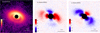 |
Fig. 1 Left to right: IRDIS total intensity K-band, Stokes Q - K-band, and Stokes U - K-band images observed from VLT-SPHERE. |
3 Analysis
In this section, we combine SPHERE/IRDIS Ks-band scattered light images with ALMA continuum images to obtain a self-consistent model of LkCa 15 that can explain the disc morphology at both NIR and millimetre wavelengths. We first present the IRDIS data reduction products and construct an inverse polarisation-fraction map to search for low-polarisation companions. We then fit the disc with RADMC-3D using compact-olivine (Mie) grains in two populations, jointly constrained by IRDIS and ALMA, which sets the global geometry and reproduces the millimetre ring-gap structure. However, this compact-olivine solution leaves systematic mismatches in the Ks morphology -too little near-side brightness at small-intermediate scattering angles. To diagnose these issues quantitatively, we extract and compare the scattering and polarisation phase functions, S (θ) and p(θ), for the data as well as model them with grains of different porosity and sizes. This analysis confirms the discrepancies and motivates replacing compact spheres with porous CAHP aggregates in the near-IR scattering layer, while preserving the jointly constrained geometry. Because millimetre-wavelength optical properties for CAHP are not yet available, this refinement is applied only to the near-IR. We detail the IRDIS flux calibration, and conclude with companion-detection limits derived from disc-subtracted reductions.
3.1 IRDIS: Simultaneous polarimetry and total intensity in the K band
The IRDIS system, a component of SPHERE, has the ability to capture total-intensity and polarised-intensity images in the Y, J, H, and Ks bands. While the H band offers a superior resolution compared to the Ks band, the latter demonstrates a markedly ~10% higher Strehl ratio, especially for faint objects such as LkCa 15 (R = 11.61). Consequently, we chose to image the LkCa 15 proto-planetary disc in the Ks band. Figure 1 shows the total intensity image together with the polarimetric Q and U images, while Figure C.1 (in Appendix C) shows the Qφ and Uφ images.
From the total intensity and polarisation images, we proceeded to estimate the inverse polarimetric fraction map,  , which could potentially reveal planets with a low polarisation signal. Planetary atmospheres usually scatter light with much lower polarisation fraction than discs (also see van Holstein et al. (2021). Therefore, in a polarisation fraction map, planets would normally appear as intensity dips. Here, we use inverse maps so that planets show up as bright spots on the dark background. To ensure that the map is not dominated by noise in regions with low
  , we set these region’s pixels to a constant value. This constant was three times the standard deviation (σ) of
  in a background annulus with no significant signal. This was done for regions with
  . However, even with this method, we do not find any strong planetary signatures in the LkCa 15 image shown in Figure 2. Note that our method can only detect planets if a low-polarisation planet is superimposed on a high-polarisation disc and detected with a robust signal-to-noise ratio (S/N).
3.2 Radiative transfer modelling of the LkCa 15 disc
We used the radiative transfer code RADMC-3D (Dullemond et al. 2012) to study the properties and structure of the LkCa 15 proto-planetary disc. With RADMC-3D, we were able to generate models of the observed morphology of the disc at different wavelengths of the spectrum, i.e. scattered light with polarimetry at 2.2 μm (SPHERE data) and thermal emission at sub-milimetre wavelengths (ALMA data). These datasets provide complementary information about the disc, with SPHERE probing the surface layers dominated by micron-sized grains and ALMA revealing the disc mid-plane driven by millimetre-sized grains.
The main goal of this modelling is to create a self-consistent disc model that can explain both scattered light and thermal emission. By constraining key parameters such as the disc geometry, grain size distribution, and flaring, we aim to infer the physical structure and composition of the LkCa 15 disc. Our modelling framework involved defining the physical and geometrical properties of the disc and generating synthetic model images that could be directly compared with observations. Through an iterative process of refining the models and comparing them with observational data, we tried to find the best-fit solution that aligns with the observed morphology.
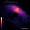 |
Fig. 2 Inverted K-band polarisation fraction ( |

3.2.1 Model assumptions and parameters
The radiative transfer model incorporates several physical assumptions about the disc’s structure, dust properties, and scattering behaviour. Key aspects are outlined below:
Scattering theory and dust grain properties: dust grains are assumed to follow a power-law size distribution, n(a) ∝ aζ, with sizes ranging from sub-micron to millimetre scales. This size distribution ensures that the model captures the effect of both small grains, which dominate scattered light and polarisation at shorter wavelengths, and larger grains, which are the primary contributors to sub-millimetre thermal emission. The optical constants for the compact Mie grains were adopted from Dorschner et al. (1995), while those for the irregular porous grains were taken from Tazaki & Dominik (2022). Because we supplied pre-computed opacity files for each representative grain size computed using OP-TOOL (Dominik et al. 2021), RADMC-3D treated each file as an independent dust species and ignored the gsmin (minimum grain size), gsmax (maximum grain size), and other grain distribution parameters, which only apply when opacities are generated internally from optical constant files (see Dullemond et al. (2012) for more details).
Disc geometry: the disc was modeled as an axisymmetric structure defined by its inner and outer radii (rin, rout), inclination (i), and position angle (PA).
Surface density distribution and gaps: each annular zone was assigned an independent power-law surface density, Σ(r) ∝ r−plsig, between its inner and outer radii (Rin, Rout). Where needed, we imposed an explicit depletion gap using the RADMC-3D controls gap_rin, gap_rout, and gap_drfact. Inside the interval r ∈ [gap_rin, gap_rout], the surface density is multiplied by gap_drfact (<1 for a depletion). Gaps are specified independently for each zone; leaving them unset (or gap_drfact=1) disables the depletion for that zone.
-
Vertical density profile and flaring: we assumed a Gaussian vertical density distribution,
![Mathematical equation: \rho(r,z) \;=\; \rho_0(r)\,\exp\Bigl[-\tfrac12\bigl(z/H(r)\bigr)^2\Bigr],](/articles/aa/full_html/2026/02/aa49743-24/aa49743-24-eq7.png)
where the pressure scale height is

Here H0 is the aspect ratio, H/r, at the pivot radius, Rpiv , and ‘plh’ is the flaring exponent. Thus at r = Rpiv one recovers H(Rpiv) = H0 Rpiv. Although we did not compute a full gas density profile, we used the pressure scale height, H(r), to prescribe the disc’s vertical thickness and flaring, thereby defining its three-dimensional geometry for radiative transfer. For our RADMC-3D models, we chose the Rpiv at 50 au.
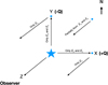 |
Fig. 3 Schematic diagram showing the axis orientation for the E field chosen in this paper. The +Q is aligned in the X direction and -Q is aligned in the Y direction. The blue points represent the dust grains, while the arrows indicate the scattered photons towards the observer, an incomparably large distance away. |
3.2.2 The polarimetric images
RADMC-3D has the capability to generate polarimetric images (Stokes: Q, U) along with the intensity images. Because the axes used to define the components of the electric field vectors are arbitrary, the appearance of the Q and U images also varies depending on the chosen convention. To make the images obtained from IRDAP and RADMC-3D consistent with each other, for both images we defined the axis of the E field relative to the north as is shown in Figure 3. The positive Q (+Q) is oriented in the X direction, whereas the negative Q (-Q) is aligned in the Y direction. A photon emitted from the star, as an electromagnetic wave, has no electric field component in its direction of propagation. Consequently, the electric field is confined to the two orthogonal directions. If a photon approaches the particle in the Y direction, its electric field will have Ex and Ez components. After scattering towards the observer in the Z direction, only the Ex component will be preserved. Similarly, if the photon approaches in the X direction, then only Ey will be preserved. At intermediate angles, both Ex and Ey components contribute, with Q>0 if Ex>Ey, and Q<0 if Ex<Ey. For an inclined disc, the orientations of the Ex and Ey components vary, resulting in uneven positive regions (red) in the east-west direction and negative regions (blue) in the north-south direction.
Similar to the Q images, the U images also exhibit positive and negative regions, which are represented in a similar manner as is illustrated in Figure 4. Since the orientation of the +Q and -Q is arbitrary, different models and reduction tools may use different directions to represent +Q and -Q. Therefore, it is necessary to apply a suitable corrections before comparing the images. For example, the orientation of the images obtained from IRDAP pipeline and RADMC-3D has an offset of +90° clockwise, and thus a proper alignment is necessary before a comparison. The second and third rows in Figure 5 show both the observed and modelled polarimetric images for the LkCa 15 after applying the offset correction. We find that the orientation of the positive and negative regions of the Q and U image and the model are correct, though there is a considerable residual for both cases. A circular mask of radius ~20 au has been applied both to the data and the model to block the central PSF, which is necessary for the scattered light images. Since we mask the inner ~20 au of the disc, we exclude regions where PSF convolution could artificially alter the polarisation signal from unresolved sub-FWHM structures. The SPHERE/IRDIS Ks-band PSF has a FWHM of ~50mas (corresponding to ~7.85 au at 157 pc), so our mask spans nearly three times the PSF width. As a result, smallscale polarimetric features susceptible to PSF-induced artefacts (Heikamp & Keller 2019; Tschudi & Schmid 2021; Ma et al. 2024) are already excluded from both the modelling and the χ2 computation, justifying our approach.
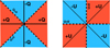 |
Fig. 4 Signs of Stokes parameters taken in this paper indicating the positive and negative regions in Q and U images. |
3.2.3 Flux calibration
We converted the IRDIS images in ADU units to flux density in Jansky (Jy) using the known K-band flux density of LkCa 15 ( F* = 0.369 Jy; Cutri et al. (2003). First, we performed aperture photometry on the non-coronagraphic frames to measure the stellar count rate. We then scaled this by the filter transmission accounting for the neutral density (ND) filter attenuation and by the exposure time (DIT) to establish a conversion factor from ADU to Jy, CPS* (in ADU s−1). Finally, the coronagraphic disc flux (Fdisc [Jy]) was computed as
 (1)
(1)
where ADUdisc is the disc signal in detector counts (after subtracting background and stellar PSF), and DITdisc is the detector integration time (DIT) or the exposure time of a single frame.
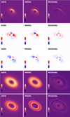 |
Fig. 5 Comparison of RADMC-3D model with olivine grains and observed data. The sequence from left to right shows the data, the simulated model, and the residuals. The top row is the K-band total intensity image, followed by the K-band Stokes Q, and the Stokes U. The fourth and fifth rows at the bottom correspond to ALMA 880 μm and 1300 μm images, respectively. |
3.2.4 Radiative transfer modelling with compact olivine Mie spheres
To model the proto-planetary disc in scattered light and at submillimetre wavelengths, we adopted a minimal two-population dust model with micron-sized grains in the surface layer and millimetre-sized grains in the mid-plane. In the ALMA images, the disc appears geometrically thin because the thermal continuum is dominated by large grains that have settled toward the mid-plane (Pinte et al. 2016). In contrast, the SPHERE NIR images trace a significantly flared, three-dimensional scattering surface (Fig. 5), which requires small grains. A single grain population cannot reproduce both the flat millimetre continuum and the flared NIR morphology, which motivates our two-component dust prescription.
As is discussed in Sect. 2, we modelled the LkCa 15 proto-planetary disc using SPHERE Ks-band (2.2 μm) Stokes I, Q, and U images together with the ALMA 880 μm and 1300 μm continuum maps. The model images were first scaled to the observed images by minimising the root mean square (RMS) difference in an annulus between 10 and 75 pixels. We then evaluated a mean reduced image chi-square,  , which measured the agreement in morphology after this renormalisation, and a separate flux chisquare,
  , which compared the integrated fluxes in the NIR and ALMA bands (see Appendix D). The total reduced chi-square was defined as
  , but in practice we first searched for good solutions by minimising
  alone, as this was computationally faster; we then used χR to refine the fit once an acceptable morphological match had been found.
For the NIR total disc flux, we adopted a conservative 15% uncertainty, following Wahhaj et al. (2024). This budget accounts for the dominant SPHERE systematics; namely, absolute photometric calibration uncertainties (−5−10%), neutraldensity filter transmission (~3%), flat-field and backgroundsubtraction residuals (−3%), and star-hopping PSF-subtraction uncertainties (~5—10%) (SPHERE Manual 2024). For the ALMA 880 μm and 1.3 mm data, we assumed flux uncertainties of the order of 10%, so that the millimetre continuum provides much tighter constraints on the total flux than the NIR images. The resulting values of  and
and  for our best-fit model are listed in Table D.1.
Our best-fit olivine model (Fig. 5) consists of a micron-sized surface layer extending from −25 au to 85 au and a millimetreemitting ring from −55 au to 130 au, with a prominent gap between −75 au and 100 au in the latter. The overall disc geometry is well reproduced, with an inclination of inc ≈ −50° and a position angle of PA ≈ 61.5°. Following Dorschner et al. (1995), we adopted amorphous olivine with a 50:50 forsterite-fayalite composition (equal fractions of Mg2SiO4 and Fe2SiO4). The corresponding best-fit parameters for the micron and millimetre components are listed in Table 3, and a schematic view of the resulting disc structure is shown in Fig. 6.
The two representative grain sizes used in this model (12 μm and 2 mm) were not chosen a priori but treated as free parameters in an iterative χ2 minimisation with RADMC-3D. Grain sizes of −12 μm provide the best match between total intensity and polarisation in the SPHERE Ks band, reproducing both the moderately forward-scattering phase function and the observed surface-brightness distribution; in contrast, sub-micron grains yield polarised intensities that are too low, while larger (>20 μm) grains produce phase functions that are overly peaked at small scattering angles. For the ALMA 880 μm and 1.3 mm continuum, the observed fluxes and ring morphology are best matched by grains of the order of 1-2 mm, with a best fit size of −2 mm that minimises the residuals. These two grain sizes should therefore be regarded as effective representatives of the dominant scattering and emitting populations at the disc surface and in the millimetre-emitting mid-plane, respectively.
Despite reproducing the overall geometry and the ring-gap structure seen in the ALMA images, the compact-olivine model shows clear shortcomings in the SPHERE Ks-band scattered light. The residuals in Fig. 5 reveal that the inner disc in the total intensity model is too strongly forward-scattered compared to the observations, and the spatial distributions of the Stokes Q and U lobes are not well reproduced. In particular, the observed polarised intensity shows more emission at large scattering angles (on the far side of the disc) than our compact 12 μm Mie grains can generate. Because these grains produce a highly forward-peaked phase function with relatively weak backward scattering, they are unable to match the detailed polarimetric structure of the SPHERE data even though they reproduce the ALMA continuum rings. This, in turn, motivates the exploration of alternative dust models, which we present in the next subsection; there we show that CAHP-128-100,nm grains yield the closest agreement with the observed polarisation phase curves of the LkCa 15 disc.
Best-fit parameters using the olivine grains.
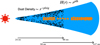 |
Fig. 6 Schematic diagram of our LkCa 15 proto-planetary disc with olivine grains. The black and orange represent the micron- and millimetre-sized grains, respectively. |
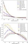 |
Fig. 7 Comparison of the SPHERE Ks-band scattered light phase function (red points) to a family of CAHP aggregate grain models with monomer counts 16, 32,..., 1024 (solid coloured lines), and to a compact ~ 8 μm olivine grain (dashed pink). Top : normalised scattered-light intensity (flux) as a function of scattering angle. Bottom : polarised phase function versus scattering angle for the same model series and data points. |
3.2.5 Scattering phase function and polarisation diagnostics
To constrain the size and structure of the dust grains responsible for NIR scattering in the LkCa 15 disc, we used diskmap2 (Stolker et al. 2016) to extract both the scattering phase function and polarisation fraction from our Ks-band observations at a deprojected radius between 35 and 70 au. These diagnostics directly characterise the angular distribution of scattered light and the degree of polarisation as functions of scattering angle, bypassing the complexities of absolute flux calibration and multi-zone radiative transfer. The diskmap tool mapped each pixel in our scattered-light images to a corresponding scattering angle, based on the three-dimensional geometry of the LkCa 15 disc. This enabled us to construct the total intensity phase function, S (θ), and polarisation fraction, P(θ), as a function of the scattering angle, θ. For comparison with theoretical models, we normalised the phase function such that flux = 1, setting the intensity at θ = 90° as a reference point. From the normalised intensity flux plot as shown in Figure 7, our analysis reveals that S (θ) shows a moderate forward-scattering enhancement, increasing by a factor of ~5 from 90° to 35°. This behaviour is more forward-peaked than for ideal Rayleigh scatterers (submicron grains), but less extreme than expected for compact, micron-sized spheres, which would produce a much sharper forward-scattering peak as is seen in the case of olivine. From the P(θ) plot in Figure 7, the observed data points (red) show a broad peak near θ ~ 70° and decline at both smaller and larger angles, with an amplitude and shape that cannot be reproduced by compact olivine grains or pure Rayleigh scatterers.
To interpret these findings, we compared the extracted phase curves to theoretical models generated with AggScatVIR3 (Tazaki & Dominik 2022; Tazaki et al. 2023), which simulates scattering by porous aggregate grains composed of sub-micron monomer clusters. We tested several classes of aggregates, such as fractal aggregates (FAs) and compact aggregates (CAs), with low porosity (LP), medium porosity (MP), and high porosity (HP) models and varying the number of monomers and grain size. Among these, the CAHP-128-100 nm model, representing an aggregate of 128 monomers (each with 0.1 μm radius) and a porosity of −87%, provides the closest match to the observed phase function and polarisation fraction, as is seen in Figure 7. This model successfully reproduces both the moderate forward-scattering enhancement in S (θ) and the reduced, flattened polarisation peak in P(θ). The polarisation fraction,  , displays a broad maximum near θ ~ 90°, with a peak value of ~0.35, and decreases at smaller and larger angles. This peak is significantly lower than the Rayleigh limit (P(θ) = 1) as shown in Figure 9, implying that the grains responsible for the observed scattering are outside the Rayleigh regime and/or possess irregular, aggregate structures.
By combining disc geometry derived from RADMC-3D with the diskmap-based phase extraction and aggregate grain modelling using AggScatVIR, our analysis provides robust, independent confirmation that the scattering surface of LkCa 15 is dominated by porous, micron-scale aggregates with moderate anisotropy and polarisation efficiency. Thus we decided to perform our RT modelling for our disc with CAHP-128-100 nm grains.
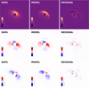 |
Fig. 8 Side by side comparison between the observations and a RADMC-3D model with CAHP-128-100nm grains, plus residuals. Left to right: data, model, residuals. Rows (top to bottom): K-band total intensity, Stokes Q, and Stokes U. We did not model the ALMA images using CAHP grains as we do not have the optical properties of the CAHP grains at millimetre wavelengths. |
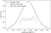 |
Fig. 9 Polarisation fraction as a function of scattering angle for the LkCa 15 disc. Red points: SPHERE Ks-band data (debiased). Blue: CAHP-128-100 nm high-porosity aggregate model. Dashed black: Rayleigh limit. The broad, sub-Rayleigh peak indicates that scattering is dominated by porous aggregate grains rather than compact Mie spheres. |
3.2.6 Radiative transfer modelling with CAHP grains
The compact olivine Mie model does not reproduce the observed Ks -band morphology as it fails to match the near-side brightness at small scattering angles in Stokes I and yields ansae with too low contrast in Stokes Q and U (Fig. 5). To test whether this mismatch arises from the scattering physics of the surface grains, we replaced compact spheres in the NIR scattering layer with irregular porous aggregates and recomputed the models under identical assumptions for geometry, grid, wavelength sampling, image masks, and PSF treatment. Following the analysis in Sect. 3.2.5, we adopted CAHP-128-100 nm grains, which provide the best match to the measured scattering phase function and polarisation fraction, and we ingested the corresponding scattering matrices into RADMC-3D. We then performed the same χ2 minimisation procedure as in Sect. 3.2.4. The best-fit CAHP model preserves the global geometry, with an inclination of about 49° and a position angle of 61° as shown in Figure 8. The NIR scattering layer extends from ~25-85 au with modest flaring (plh = 1.17) and H/R ≈ 0.08 at 50 au. A shallow gap is recovered from ~ 36 to 42 au with a depletion factor of 0.41, and the surface-layer dust mass is 2 × 10⁻⁵ M⊙ (Table 4).
With CAHP aggregates the Ks-band morphology improves in both total intensity and polarimetry. The near-side inner arc becomes brighter and more structured, reducing the residuals seen with compact olivine spheres, and the ansae in Stokes Q and U become sharper, allowing us to reproduce the ‘ear’-like lobes seen in the SPHERE data. Quantitatively, the mean reduced χ2 for the scattered-light images decreases from 1.58 in the compact-olivine model to 1.34 in the CAHP case, and the individual reduced χ2 values for the NIR images improve from 1.36, 1.45, and 1.93 (Stokes I, Q, and U) to 1.06, 1.24, and 1.74, respectively. The fractional flux differences likewise shrink from 14/34/43% to 11/8/3% for I/Q/U (Table D.1). We therefore conclude that irregular porous aggregates provide a significantly better description of the NIR scattering layer than compact Mie spheres. These improvements, however, apply only to the SPHERE Ks-band scattered light, as the ALMA 880 μm and 1.3 mm images are not modelled with CAHP grains.
This restriction reflects the current limitations of the CAHP optical-property libraries. They provide validated scattering matrices for sub-micron to micron-sized aggregates at NIR wavelengths, but do not supply absorption and scattering opacities or full Mueller matrices for grains with sizes >3.78 μm. As a result, we cannot self-consistently model the ALMA 880 μm and 1.3 mm continuum, which is dominated by absorption from settled millimetre-sized grains.
Finally, our radiative-transfer modelling is affected by parameter degeneracies, particularly between the pressure scale height (H0), the flaring index (plh), and the surface-density slope (plsig). These quantities are correlated: changes in one can often be compensated for by adjustments in the others. For example, increasing H0 can be offset by decreasing plh or increasing plsig, producing very similar apparent disc morphologies, and analogous trade-offs exist between plh and plsig. As a result, the best-fit values of these structural parameters are not uniquely constrained and should be interpreted with caution when examining the detailed numbers in Tables 3 and 4.
Best-fit parameters using the CAHP-128-100 nm dust grains.
3.2.7 Constraints on model parameters
Determining the uncertainty of our model parameters is a challenging task due to the high computational cost of Monte Carlo Bayesian estimations. Each model takes approximately one minute to compute, mainly because of the high resolution of our dataset. A representative MCMC run with 50 walkers and 1000 iterations would therefore require of the order of ~1000 hours. Using shorter runs does not provide reliable constraints on our parameters, as is shown in Appendix D of Wahhaj et al. (2024). To address this issue, we adopted the methodology proposed by Wahhaj et al. (2024) to obtain an approximate estimate of the uncertainties near the local minimum. For each parameter, we calculated the best chi-squared (χ2) along a linear grid centred around the optimal fit point, allowing the other parameters to vary. To determine the uncertainty for each parameter, we chose the interval along the grid where the variation in χ2 remains within 1 % of its minimum value. We chose this threshold because our χ2 estimates had a precision of around 0.5%. It is important to note that this method does not find the global best-fit model or provide definitive uncertainties. However, it does effectively demonstrate the relative strength or weakness of the constraints around our best-fit model.
The lower and upper bounds for our models, as is shown in Tables 3 and 4, reveal that most parameters are tightly constrained at the local minimum. The inner and outer radii (Rin and Rout) critically affect the extent of the disc emission in scattered light, and thus are strongly constrained. The dust mass (Mdust) is well constrained, as it strongly affects the optical thickness in the Ks band. The power law height (plh) and height ratio disc (H0) are moderately constrained. They show evidence of some vertical thickness observed in scattered light and less in thermal emission. The larger grains in the millimetre zone have a less pronounced effect on the observed scattered light. They significantly impact the thermal emission seen in the ALMA bands. The dust mass (Mdust) in this region is somewhat constrained as it directly affects the optical depth. The outer radius (Rout) as well as the gap location is also well constrained, as it is crucial for defining the spatial extent observed in ALMA images. Overall, parameters such as dust mass and vertical height, which directly influence the 3D appearance, the clarity of the gap, and the overall brightness of the disc, are better constrained in the sub-micron and micron zones. In contrast, plsig, which influences the millimetre zone brightness, mainly in ALMA imaging, is less tightly constrained.
3.3 Companion detection limit
For LkCa 15, we did not detect any planets either in the total-intensity or in the inverted polarimetric images. Detecting planets is challenging when the proto-planetary disc is very bright, as in the case of LkCa 15. Nonetheless, we attempted to search for planets that might be hidden in the disc by removing the disc signal. This involved creating a median-smoothed version of the disc using an 8-pixel box size (twice the typical planet PSF extent of ~4 pixels, i.e. ~0.048″), which we then subtracted from the original image together with the reference star PSF, as is detailed in Section 2. Although we successfully suppressed a significant fraction of the disc emission, residuals remain, as is evident in Figure 10. Despite this partial removal, no new planet was detected.
In spite of the visual non-detection of planets, we placed upper mass limits on unseen companions by deriving a 5,σ contrast curve from the disc-subtracted image (Figure 10). To create this image, we first applied a 4-pixel box median filter to our bestfit disc model, then re-ran the LOCI algorithm using a composite reference PSF made up of the stellar PSF plus the filtered disc. Finally, the 5,σ contrast at each radius was computed as the standard deviation within an annulus, normalised by the peak stellar flux measured from 2-second exposures of LkCa 15. The contrast curve as a function of angular separation is shown in Figure 11. Using DUSTY models and assuming an age of ~1 Myr for the system (Swastik et al. 2021), we estimated the upper mass limits for planets based on the contrast magnitude, as shown on the right-hand y axis of Figure 11. We can detect planets more massive than 2.5 MJ outside ~20 au and 1.5 MJ outside 50 au. The deepest contrast is achieved between ~200 and 250 au, where the detection limit is ~1.36 MJ. However, the disc around LkCa 15 is very bright and the detection limit across the brightest part of the disc is around 3.62 MJ, so planets may remain hidden in regions of strong disc emission. It is important to note the considerable uncertainty (~5 Myr) in age estimates for such young systems, which in turn affects the reliability of companion mass limits derived from evolutionary models.
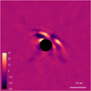 |
Fig. 10 Left : IRDIS K-band reduction with LOCI algorithm after removing most of the disc in order to detect obscured planets and to estimate the contrast limit as shown in Figure 11. |
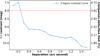 |
Fig. 11 5σ contrast curve in the K band obtained by removing the LkCa 15 proto-planetary disc. The dashed red line represents the detection limit at the brightest part of the discs. The mass estimates for the companions were obtained using DUSTY models assuming the stellar age to be 1 Myr for LkCa 15. |
4 Discussion
Based on the evidence from the scattering phase function, we have found reasonable models for our proto-planetary disc LkCa 15 both in the scattered light as well as in the millimetre regime. We find that the smaller micron-sized grains are mainly in the inner region of the disc, while the millimetresized grains mainly populate the outer part of the disc from 58 au extending till 127 au. Thus, the radial segregation of the grains is clearly evident for our proto-planetary disc, which is quite unusual as larger grains are expected to lie closer to the central star (Birnstiel & Andrews 2014). This radial segregation of grain sizes in the disc could be attributed to some key mechanisms: a) there is more thermal energy close to the star, which hinders the formation of larger grains (Pollack et al. 1996; Blum & Wurm 2008), b) the segregation of small and large dust grains is significantly influenced by gas pressure gradients (de Juan Ovelar et al. 2012). These gradients arise from variations in the disc’s gas density and temperature. Larger grains, being less coupled to the gas, drift towards regions of higher pressure where they get trapped. This occurs because pressure-supported gas needs less centrifugal force, and thus less rotational velocity. The slow gas is like a ‘headwind’ causing the large grains to drift inwards (Weidenschilling 1977). However, they can encounter pressure maxima in the disc (regions of higher gas pressure) that act as barriers, trapping them and preventing further inward migration (Pinilla et al. 2012). This trapping can occur at locations such as: a) the edges of gaps in the disc carved by planets (Paardekooper & Mellema 2006); b) snowlines (e.g. the water snowline) where the gas density and temperature change sharply (Vericel & Gonzalez 2020). On the other hand, smaller grains, which are more tightly bound to the gas, continue to follow its motion without being significantly affected by these pressure variations. This differential behaviour leads to the observed segregation, with larger grains accumulating in high-pressure areas, a key factor in planetesimal formation (Birnstiel et al. 2010; Meheut et al. 2012; Swastik et al. 2022, 2023, 2024). However, recent ALMA surveys of gas tracers in LkCa 15 challenge scenarios involving strong pressure bumps. Leemker et al. (2022), using 13CO and C18O J=2-1 data, report that the gas surface density inside the ~45-60 au dust gap drops by only a factor of ~2, which is far less than expected for a deep planet-carved cavity. Complementary 12CO J=3-2 observations from the exo-ALMA survey (Gardner et al. 2025) show a radially smooth gas distribution, even within the dust cavity, without evidence of a sharp depletion. These findings indicate that any pressure maxima in LkCa 15 are relatively modest and unlikely to be caused by a single, massive planet. Instead, the observations favour multiple lower-mass planets creating gentle pressure variations, or alternative, non-planetary mechanisms that maintain gas continuity while enabling partial dust segregation.
In addition to reproducing the disc’s morphological features, our analysis of the scattered-light phase function and polarisation fraction provides crucial, independent constraints on the physical properties of the grains at the disc surface. By extracting the scattering phase function from our Ks-band images using diskmap, we find that neither pure Rayleigh scatterers (i.e. submicron grains) nor compact micron-sized grains can account for the observed shape and amplitude of the phase curves. Instead, a comparison to theoretical models of porous aggregates with varying porosity and monomer number reveals that the disc’s surface is best described by fluffy, micron-scale aggregate grains, specifically the CAHP-128-100 nm model, which consists of 128 sub-micron monomers and ~87% porosity. This population successfully reproduces both the moderate forwardscattering enhancement and the broad, sub-Rayleigh polarisation peak observed, further supporting a scenario in which aggregate growth and porosity, not just size, are key in shaping the observable disc properties.
The classical collisional-cascade model of Dohnanyi (1969), originally developed for asteroidal and dust populations, predicts that the steady-state size distribution follows a power law,
 (2)
(2)
where dN/da is the number of particles per unit size interval, a is the particle size, and ζ is the power-law exponent. In an equilibrium state in which collisional fragmentation and coagulation balance each other, Dohnanyi found ζ = −3.5. Although this model formally applies to gas-free collisional cascades, it has become a standard benchmark because ζ = −3.5 successfully reproduces the grain-size distributions inferred for debris discs and the diffuse ISM (Dohnanyi 1969; Mathis et al. 1977), where the absence of gas makes the collisional physics comparatively simple and well constrained.
For our olivine model, with representative grain sizes of 12 μm and 2000 μm, the number ratio of grains predicted by Equation (2) for the canonical slope ζ = −3.5 is smaller by a factor of ~2 × 10⁵ than the ratio implied by our best-fit model between these two populations. Treating these sizes as sampling a single power law, reproducing the measured ratio requires a much flatter slope of ζ ≃ −2.31. In a gas-rich proto-planetary environment such as LkCa 15, such a departure from the Dohnanyi value is not unexpected: gas drag, reduced collision velocities, efficient growth of larger aggregates, and radial drift can all act to deplete small grains and enhance the abundance of millimetre-sized particles (e.g. Birnstiel et al. 2010; Testi et al. 2014). Our inferred ζ ≃ −2.31 is comparable to the shallower sub-micron-to-sub-millimetre slope (ζ ~ −2.7) recently derived for PDS 70 (Wahhaj et al. 2024), suggesting that flattened size distributions between micron and millimetre scales may be a common feature of gas-rich discs rather than an anomaly specific to LkCa 15.
Material properties may also contribute to this deviation. Classical Dohnanyi cascades assume asteroidal material composed of silicates, nickel, and iron, whereas our radiative-transfer models use amorphous olivine grains. Differences in composition and tensile strength can influence collisional outcomes and fragment size distributions. Wahhaj et al. (2024) proposed several explanations for the apparent lack of small grains in PDS 70, including the migration of sub-micron grains into the disc gap and accelerated growth of millimetre grains in the mid-plane. The latter mechanism naturally increases the relative abundance of millimetre-scale grains and flattens the size distribution between microns and millimetres, qualitatively consistent with our inferred slope. In Figure 12, the blue points represent grain sizes sampled from a distribution inferred from our model dust masses; grain-size and mass uncertainties are propagated via a Monte Carlo approach with an asymmetric Gaussian distribution, following Appendix F of Wahhaj et al. (2024). Extending this kind of joint imaging-plus-size-distribution modelling to a larger sample of proto-planetary discs will be essential to determine whether shallow slopes such as ζ ≃ −2.3 are typical in gas-rich systems.
While we successfully obtained an artefact-free image of LkCa 15, previous claimed detections of proto-planets within this system remain unconfirmed (Currie et al. 2019). This raises a key question, of whether the planets are hidden or whether the system is too young or not massive enough for the formation of massive giant planets. The brightness of our disc also limits our detection capabilities in the disc-dominated regions, as can be seen from the contrast curve in Figure 11. In comparison to systems such as PDS 70, LkCa 15 is considerably younger, with an estimated age of approximately 1-2 Myr. Since both PDS 70 and LkCa 15 are pre-main-sequence stars and have proto-planetary discs and are thus in a similar evolutionary stage, by assuming a mass accretion rate for LkCa 15 equal to that of PDS 70 (Wagner et al. 2018), a range from 10−8 MJ/yr to 10−7 MJ/yr, we infer that the maximum mass of a forming planet in this system would be around 0.2 Mj. Although this method of estimating planetary mass is somewhat oversimplified, it suggests that planets within LkCa 15 could be in the early stages of formation and may still be too small to be detected by high-contrast imaging techniques.
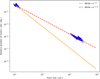 |
Fig. 12 Figure illustrates the model-estimated relative abundances of three grain sizes, compared to those predicted by the power law by Dohnanyi (1969). The data pairs were generated a Monte Carlo simulation with an asymmetric Gaussian distribution (see Section 4 for more details). |
5 Conclusions
In this work, we obtained Ks-band total-intensity and polarised-intensity images of the LkCa 15 proto-planetary disc using the star-hopping RDI technique. Our observations capture the intrinsic disc intensities for the first time, without the artefacts present in previous ADI-based observations. The primary goals of this work were: (a) to search for new planets in the ~20-30 au region using both total-intensity images and fractional-polarisation maps, and (b) to understand the disc morphology and probable dust composition. We analysed the scattering phase function and performed radiative-transfer modelling with RADMC-3D. In particular, we attempted to reproduce the total- and polarised-intensity images as well as the ALMA millimetre continuum in order to obtain a complete picture of the disc. We were able to constrain most of the observed disc morphology. We summarise the key findings as follows:
We first modelled the disc with micron- and millimetre-sized olivine grains. This set-up reproduces the total-intensity Ks-band image and the ALMA continuum reasonably well, but the scattered-light images are too strongly forward-scattering and too faint on the back side compared to the data;
The observed intensity and polarisation phase curves are inconsistent with pure Rayleigh scatterers or compact olivine grains. Instead, they are best matched by the CAHP-128-100 nm porous-aggregate model from AggScatVIR, indicating that the disc surface is dominated by fluffy, micron-sized aggregates;
Using CAHP-128-100 nm grains, guided by the scattering phase function, our model reproduces the key observed morphological features in scattered light, including the ear-like lobes in the Q and U images and the observed level of forward scattering that olivine grains could not match;
Our best-fit model consists of a micron-grain surface layer from 25-85 au and a millimetre-grain mid-plane ring from 55-130 au;
From the number ratio between the ~12 μm and ~2 mm grain populations, we infer an effective size-distribution slope of ζ ≃ −2.3, implying that micron-sized grains are under-abundant compared to ISM and/or debris-disc-like distributions;
There may be radial drift in the dust grains, with small grains lying mainly within the inner 50 au of the disc, while the outer part of the disc is mainly composed of larger millimetre-sized grains. This radial segregation is unusual relative to standard expectations of grain growth and drift;
We analysed the inverted polarised-intensity map but did not find any discernible planetary signatures in the high-S/N regions of the disc;
We could not detect any planets in the total-intensity images either. Despite not detecting new planets within the disc, we estimated upper mass limits for potential planets: planets more massive than 1.4 MJ are unlikely to exist beyond 200 au, whereas the inner brighter disc regions may conceal planets up to ~3.6 MJ.
In conclusion, compact olivine grains provide a good overall joint fit to the near-IR and millimetre data, while porous CAHP-128-100 nm aggregates are required to reproduce the near-IR scattering phase function and scattered-light morphology. Since CAHP opacities are not yet available at millimetre wavelengths, modelling the ALMA continuum with CAHP grains must await future opacity calculations.
We acknowledge the non-uniqueness of these solutions, given the degenerate nature and interplay of various parameters such as flaring, surface-density distribution, and pressure scale height. Furthermore, it is difficult to determine the dust grain composition of proto-planetary discs from imaging observations alone. Therefore, future efforts should aim for spectroscopic observations, which can provide more direct constraints on grain composition.
Finally, while we successfully obtained self-subtraction-free images of LkCa 15, previous claimed detections of protoplanets in this system remain unconfirmed. Given the youth of the system and the strong disc brightness, any embedded planets may still be in an early growth phase and below current detection limits.
It is also crucial to recognise the computational limitations in determining the optimal solution. The long model computation times pose a challenge, confining us to the discovery of the best solution around local minima rather than the true global best-fit solution. Moreover, accurate modelling and predictions of proto-planetary disc morphology are impaired by uncertainties in the underlying physical conditions. Despite these caveats, our simple radiative-transfer model accounts for the main features observed in LkCa 15.
Data availability
The final data products in fits format are available at the CDS via https://cdsarc.cds.unistra.fr/viz-bin/cat/J/A+A/706/A312
Acknowledgements
S.C. is funded by the European Union (ERC, UNVEIL, 101076613). Views and opinions expressed are however those of the author(s) only and do not necessarily reflect those of the European Union or the European Research Council. Neither the European Union nor the granting authority can be held responsible for them. S.C. acknowledges financial contribution from PRIN-MUR 2022YP5ACE. This project has received funding from the European Research Council (ERC) under the European Union’s Horizon 2020 research and innovation programme (ERC, PROTOPLANETS, 101002188). This project received funding from the Department of Science and Technology, India as PhD fellowship of C. Swastik. R.T. is supported by JSPS KAKENHI Grant Number JP25K07351.
References
- Andrews, S. M., Wilner, D. J., Zhu, Z., et al. 2016, ApJ, 820, L40 [Google Scholar]
- Avenhaus, H., Quanz, S. P., Schmid, H. M., et al. 2017, AJ, 154, 33 [Google Scholar]
- Bae, J., Zhu, Z., & Hartmann, L. 2017, ApJ, 850, 201 [NASA ADS] [CrossRef] [Google Scholar]
- Baillié, K., Marques, J., & Piau, L. 2019, A&A, 624, A93 [NASA ADS] [CrossRef] [EDP Sciences] [Google Scholar]
- Benisty, M., Bae, J., Facchini, S., et al. 2021, ApJ, 916, L2 [NASA ADS] [CrossRef] [Google Scholar]
- Beuzit, J. L., Vigan, A., Mouillet, D., et al. 2019, A&A, 631, A155 [NASA ADS] [CrossRef] [EDP Sciences] [Google Scholar]
- Birnstiel, T., & Andrews, S. M. 2014, ApJ, 780, 153 [Google Scholar]
- Birnstiel, T., Dullemond, C. P., & Brauer, F. 2010, A&A, 513, A79 [NASA ADS] [CrossRef] [EDP Sciences] [Google Scholar]
- Blakely, D., Francis, L., Johnstone, D., et al. 2022, ApJ, 931, 3 [NASA ADS] [CrossRef] [Google Scholar]
- Blum, J., & Wurm, G. 2008, ARA&A, 46, 21 [CrossRef] [Google Scholar]
- Boccaletti, A., Mâlin, M., Baudoz, P., et al. 2024, A&A, 686, A33 [NASA ADS] [CrossRef] [EDP Sciences] [Google Scholar]
- Bonnefoy, M., Zurlo, A., Baudino, J. L., et al. 2016, A&A, 587, A58 [NASA ADS] [CrossRef] [EDP Sciences] [Google Scholar]
- Canovas, H., Ménard, F., de Boer, J., et al. 2015, A&A, 582, L7 [NASA ADS] [CrossRef] [EDP Sciences] [Google Scholar]
- Casassus, S., Perez M. S., Jordán, A., et al. 2012, ApJ, 754, L31 [NASA ADS] [CrossRef] [Google Scholar]
- Claudi, R. U., Turatto, M., Gratton, R. G., et al. 2008, SPIE Conf. Ser., 7014, 70143E [Google Scholar]
- Currie, T., Marois, C., Cieza, L., et al. 2019, ApJ, 877, L3 [Google Scholar]
- Currie, T., Lawson, K., Schneider, G., et al. 2022, Nat. Astron., 6, 751 [NASA ADS] [CrossRef] [Google Scholar]
- Cutri, R. M., Skrutskie, M. F., van Dyk, S., et al. 2003, VizieR Online Data Catalog: 2MASS All-Sky Catalog of Point Sources (Cutri+ 2003), VizieR On-line Data Catalog: II/246. Originally published in: 2003yCat.2246....0C [Google Scholar]
- de Boer, J., Langlois, M., van Holstein, R. G., et al. 2020, A&A, 633, A63 [NASA ADS] [CrossRef] [EDP Sciences] [Google Scholar]
- de Juan Ovelar, M., Kruijssen, J. M. D., Bressert, E., et al. 2012, A&A, 546, L1 [NASA ADS] [CrossRef] [EDP Sciences] [Google Scholar]
- Dipierro, G., Price, D., Laibe, G., et al. 2015, MNRAS, 453, L73 [NASA ADS] [CrossRef] [Google Scholar]
- Dohlen, K., Langlois, M., Saisse, M., et al. 2008, SPIE Conf. Ser., 7014, 70143L [Google Scholar]
- Dohnanyi, J. S. 1969, J. Geophys. Res., 74, 2531 [Google Scholar]
- Dominik, C., Min, M., & Tazaki, R. 2021, OpTool: Command-line driven tool for creating complex dust opacities, Astrophysics Source Code Library [record ascl:2104.010] [Google Scholar]
- Dong, R., & Fung, J. 2017, ApJ, 835, 146 [NASA ADS] [CrossRef] [Google Scholar]
- Dong, R., Hall, C., Rice, K., & Chiang, E. 2015, ApJ, 812, L32 [Google Scholar]
- Dorschner, J., Begemann, B., Henning, T., Jaeger, C., & Mutschke, H. 1995, A&A, 300, 503 [Google Scholar]
- Dullemond, C. P., Juhasz, A., Pohl, A., et al. 2012, RADMC-3D: A multipurpose radiative transfer tool, Astrophysics Source Code Library [record ascl:1202.015] [Google Scholar]
- Espaillat, C., Calvet, N., D’Alessio, P., et al. 2007, ApJ, 670, L135 [Google Scholar]
- Espaillat, C., Calvet, N., Luhman, K. L., Muzerolle, J., & D’Alessio, P. 2008, ApJ, 682, L125 [Google Scholar]
- Esposito, T. M., Fitzgerald, M. P., Graham, J. R., & Kalas, P. 2014, ApJ, 780, 25 [Google Scholar]
- Facchini, S., Benisty, M., Bae, J., et al. 2020, A&A, 639, A121 [EDP Sciences] [Google Scholar]
- Fusco, T., Petit, C., Rousset, G., et al. 2006, SPIE Conf. Ser., 6272, 62720K [NASA ADS] [Google Scholar]
- Fusco, T., Sauvage, J. F., Petit, C., et al. 2014, SPIE Conf. Ser., 9148, 91481U [NASA ADS] [Google Scholar]
- Gaia Collaboration (Vallenari, A., et al.) 2023, A&A, 674, A1 [NASA ADS] [CrossRef] [EDP Sciences] [Google Scholar]
- Gardner, C. H., Isella, A., Li, H., et al. 2025, ApJ, 984, L16 [Google Scholar]
- Ginski, C., Stolker, T., Pinilla, P., et al. 2016, A&A, 595, A112 [NASA ADS] [CrossRef] [EDP Sciences] [Google Scholar]
- Haffert, S. Y., Bohn, A. J., de Boer, J., et al. 2019, Nat. Astron., 3, 749 [Google Scholar]
- Heikamp, S., & Keller, C. U. 2019, A&A, 627, A156 [NASA ADS] [CrossRef] [EDP Sciences] [Google Scholar]
- Isella, A., Pérez, L. M., & Carpenter, J. M. 2012, ApJ, 747, 136 [NASA ADS] [CrossRef] [Google Scholar]
- Isella, A., Chandler, C. J., Carpenter, J. M., Pérez, L. M., & Ricci, L. 2014, ApJ, 788, 129 [NASA ADS] [CrossRef] [Google Scholar]
- Jin, S., Isella, A., Huang, P., et al. 2019, ApJ, 881, 108 [NASA ADS] [CrossRef] [Google Scholar]
- Jones, M. I. 2025, The Messenger, 194, 19 [Google Scholar]
- Jones, M. I., Milli, J., Blanchard, I., et al. 2022, A&A, 667, A114 [NASA ADS] [CrossRef] [EDP Sciences] [Google Scholar]
- Juillard, S., Christiaens, V., Absil, O., Stasevic, S., & Milli, J. 2024, A&A, 688, A185 [NASA ADS] [CrossRef] [EDP Sciences] [Google Scholar]
- Keppler, M., Benisty, M., Müller, A., et al. 2018, A&A, 617, A44 [NASA ADS] [CrossRef] [EDP Sciences] [Google Scholar]
- Kraus, A. L., & Ireland, M. J. 2012, ApJ, 745, 5 [Google Scholar]
- Lafrenière, D., Marois, C., Doyon, R., Nadeau, D., & Artigau, É. 2007, ApJ, 660, 770 [Google Scholar]
- Leemker, M., Booth, A. S., van Dishoeck, E. F., et al. 2022, A&A, 663, A23 [NASA ADS] [CrossRef] [EDP Sciences] [Google Scholar]
- Long, F., Andrews, S. M., Zhang, S., et al. 2022, ApJ, 937, L1 [NASA ADS] [CrossRef] [Google Scholar]
- Ma, J., Schmid, H. M., & Stolker, T. 2024, A&A, 683, A18 [NASA ADS] [CrossRef] [EDP Sciences] [Google Scholar]
- Marois, C., Lafrenière, D., Doyon, R., Macintosh, B., & Nadeau, D. 2006, ApJ, 641, 556 [Google Scholar]
- Mathis, J. S., Rumpl, W., & Nordsieck, K. H. 1977, ApJ, 217, 425 [Google Scholar]
- Meheut, H., Meliani, Z., Varniere, P., & Benz, W. 2012, A&A, 545, A134 [NASA ADS] [CrossRef] [EDP Sciences] [Google Scholar]
- Mendigutía, I., Oudmaijer, R. D., Schneider, P. C., et al. 2018, A&A, 618, L9 [CrossRef] [EDP Sciences] [Google Scholar]
- Milli, J., Mouillet, D., Lagrange, A. M., et al. 2012, A&A, 545, A111 [NASA ADS] [CrossRef] [EDP Sciences] [Google Scholar]
- Montesinos, M., Perez, S., Casassus, S., et al. 2016, ApJ, 823, L8 [Google Scholar]
- Müller, A., Keppler, M., Henning, T., et al. 2018, A&A, 617, L2 [Google Scholar]
- Oh, D., Hashimoto, J., Tamura, M., et al. 2016, PASJ, 68, L3 [Google Scholar]
- Paardekooper, S. J., & Mellema, G. 2006, A&A, 459, L17 [CrossRef] [EDP Sciences] [Google Scholar]
- Piétu, V., Dutrey, A., Guilloteau, S., Chapillon, E., & Pety, J. 2006, A&A, 460, L43 [NASA ADS] [CrossRef] [EDP Sciences] [Google Scholar]
- Pinilla, P., Birnstiel, T., Ricci, L., et al. 2012, A&A, 538, A114 [NASA ADS] [CrossRef] [EDP Sciences] [Google Scholar]
- Pinte, C., Dent, W. R. F., Ménard, F., et al. 2016, ApJ, 816, 25 [Google Scholar]
- Pollack, J. B., Hubickyj, O., Bodenheimer, P., et al. 1996, Icarus, 124, 62 [NASA ADS] [CrossRef] [Google Scholar]
- Price, D. J., Cuello, N., Pinte, C., et al. 2018, MNRAS, 477, 1270 [Google Scholar]
- Ren, B. B., Benisty, M., Ginski, C., et al. 2023, A&A, 680, A114 [NASA ADS] [CrossRef] [EDP Sciences] [Google Scholar]
- Sallum, S., Follette, K. B., Eisner, J. A., et al. 2015, Nature, 527, 342 [Google Scholar]
- Sallum, S., Eisner, J., Skemer, A., & Murray-Clay, R. 2023, ApJ, 953, 55 [NASA ADS] [CrossRef] [Google Scholar]
- Schmid, H. M., Bazzon, A., Roelfsema, R., et al. 2018, A&A, 619, A9 [NASA ADS] [CrossRef] [EDP Sciences] [Google Scholar]
- Simon, M., Dutrey, A., & Guilloteau, S. 2000, ApJ, 545, 1034 [NASA ADS] [CrossRef] [Google Scholar]
- SPHERE Manual 2024, SPHERE User Manual, accessed: 2024-10-10 [Google Scholar]
- Stolker, T., Dominik, C., Min, M., et al. 2016, A&A, 596, A70 [NASA ADS] [CrossRef] [EDP Sciences] [Google Scholar]
- Swastik, C., Banyal, R. K., Narang, M., et al. 2021, AJ, 161, 114 [Google Scholar]
- Swastik, C., Banyal, R. K., Narang, M., et al. 2022, AJ, 164, 60 [CrossRef] [Google Scholar]
- Swastik, C., Banyal, R. K., Narang, M., et al. 2023, AJ, 166, 91 [NASA ADS] [CrossRef] [Google Scholar]
- Swastik, C., Banyal, R. K., Narang, M., Unni, A., & Sivarani, T. 2024, AJ, 167, 270 [NASA ADS] [CrossRef] [Google Scholar]
- Tazaki, R., & Dominik, C. 2022, A&A, 663, A57 [NASA ADS] [CrossRef] [EDP Sciences] [Google Scholar]
- Tazaki, R., Ginski, C., & Dominik, C. 2023, ApJ, 944, L43 [NASA ADS] [CrossRef] [Google Scholar]
- Testi, L., Birnstiel, T., Ricci, L., et al. 2014, in Protostars and Planets VI, eds. H. Beuther, R. S. Klessen, C. P. Dullemond, & T. Henning, 339 [Google Scholar]
- Thalmann, C., Mulders, G. D., Janson, M., et al. 2015, ApJ, 808, L41 [Google Scholar]
- Thalmann, C., Janson, M., Garufi, A., et al. 2016, ApJ, 828, L17 [Google Scholar]
- Trapman, L., Miotello, A., Kama, M., van Dishoeck, E. F., & Bruderer, S. 2017, A&A, 605, A69 [NASA ADS] [CrossRef] [EDP Sciences] [Google Scholar]
- Tschudi, C., & Schmid, H. M. 2021, A&A, 655, A37 [NASA ADS] [CrossRef] [EDP Sciences] [Google Scholar]
- Tuthill, P., Lloyd, J., Ireland, M., et al. 2006, SPIE Conf. Ser., 6272, 62723A [Google Scholar]
- van Boekel, R., Henning, T., Menu, J., et al. 2017, ApJ, 837, 132 [Google Scholar]
- van der Plas, G., Wright, C. M., Ménard, F., et al. 2017, A&A, 597, A32 [NASA ADS] [CrossRef] [EDP Sciences] [Google Scholar]
- van Holstein, R. G., Girard, J. H., de Boer, J., et al. 2020, IRDAP: SPHERE-IRDIS polarimetric data reduction pipeline, Astrophysics Source Code Library [record ascl:2004.015] [Google Scholar]
- van Holstein, R. G., Stolker, T., Jensen-Clem, R., et al. 2021, A&A, 647, A21 [EDP Sciences] [Google Scholar]
- Vericel, A., & Gonzalez, J.-F. 2020, MNRAS, 492, 210 [NASA ADS] [CrossRef] [Google Scholar]
- Wagner, K., Follete, K. B., Close, L. M., et al. 2018, ApJ, 863, L8 [Google Scholar]
- Wahhaj, Z., Benisty, M., Ginski, C., et al. 2024, A&A, 687, A257 [NASA ADS] [CrossRef] [EDP Sciences] [Google Scholar]
- Wahhaj, Z., Milli, J., Romero, C., et al. 2021, A&A, 648, A26 [EDP Sciences] [Google Scholar]
- Wang, J. J., Vigan, A., Lacour, S., et al. 2021, AJ, 161, 148 [Google Scholar]
- Weidenschilling, S. J. 1977, MNRAS, 180, 57 [Google Scholar]
- Zurlo, A., Vigan, A., Galicher, R., et al. 2016, A&A, 587, A57 [NASA ADS] [CrossRef] [EDP Sciences] [Google Scholar]
Appendix A The star-hopping pipeline: more detections from the Ren et al. 2023 sample
The star-hopping RDI reduction for discs is done using the steps below:
Basic calibration: Flat-field, remove bad pixels, and center the raw image files to obtain the science and reference image frames as done in Wahhaj et al. (2021)
-
Reference radial profile correction: Since the reference star might not have the same brightness as the science star, the reference radial intensity profiles needs to be matched to the median science profile. We do this by multiplying a radial scaling function, α(r), to the reference frames. The radial function, α(r), is defined as:

where c1 and c2 are the fluxes of the science (median-combined images) and reference frames, respectively, at the coronagraphic edge (r = r0), and b1 and b2 are the fluxes at the AO correction radius (r = r1). The scaling ensures that α( r0) = c1/c2 and α(r1) = b1/b2, matching the fluxes at these key radii.
The power-law index, p, was determined from the radial profile of the median science frames using:

yielding:

The derived scaling function, α(r), was applied to the reference frames to match the median radial profiles of the science frames, ensuring consistency at r0 and r1.
Remove background slopes: Fit and remove an inclined plane from the science and reference images to mitigate suboptimal sky subtraction.
Identify signal and background regions:
Preliminary science reduction: Perform a LOCI PSF subtraction (Lafrenière et al. 2007) within the defined region using the most basic configuration-a full-frame, single-region with no radial or azimuthal sub-sectors so that the PSF model is derived by minimising residuals across the entire annulus in one step.
Reference-alone ADI: Perform a classical ADI reduction of the reference images independently and use the residuals as a detection limit for the LOCI science reduction. Use this detection threshold to identify signal and background regions in the science reduction.
Science cube median PSF subtraction:
Rank reference PSFs: Define a region between 8-70 pixels from the star, corresponding to the primary detection area. For each science image, perform optimally intensity-scaled subtractions with all reference images and identify those that yield an RMS within 30% of the minimum RMS in the residuals. This provides an optimal reference set for each science image, used in subsequent steps.
Make science 2nd cube: Find LOCI PSF matches for the median combination of the science frames on each side of the IRDIS detector, using the previously defined background region and the optimal references. Subtract the reference PSF match for each detector side from the corresponding science image to produce a difference cube, s1.
Make reference 2nd cube: Subtract the same reference PSF match from each reference image for its detector side to create a difference cube, r1.
Individual science PSF subtraction: Subtract LOCI PSF matches from each image in s1 using a linear combination of images in r1, restricted to the defined background region and using the optimal references, to create a difference cube, s2.
De-rotate and combine:
De-rotation and S/N calculation: De-rotate each image in s2 and calculate the S/N of the disc as the ratio of the total flux in the signal region to the standard deviation in the background region.
Median combination: Median combine the de-rotated s2 images, using only those with at least 70% of the maximum S/N.
Using the pipeline above, we were able to successfully detect four faint discs that were not reported in Ren et al. (2023) for their star-hopping observations. Thus, we present here the images of the proto-planetary discs of HD 163296 (across four epochs), SY CHA and GM AUR (see Figure A.1). We also have a disc detection for V1094, but deem it spurious. This false detection is caused by the star moving behind the coronograph by many pixels, due the differential tip-tilt loop opening. Thus, we do not shows this reduction. We point out that if the reductions show strong azimuthally symmetric arcs in the background region, it is likely due do strong remaining speckles which are rotationally smeared. If there are large smooth positive or negative regions, this is likely due to incorrect intensity scaling of the reference PSFs with respect to the science PSFs. These discs were also detected in Juillard et al. (2024) by combining ADI and RDI techniques.
The technique in Ren et al. (2023) separated circumstellar signals by flagging signal regions as “missing data” using a binary mask based on prior knowledge of their location. This ensures minimal contamination and avoids overfitting. In contrast, this work dynamically identified signal and background regions using a detection threshold obtained from a simple ADI reduction of the reference images only, requiring no prior knowledge of the signal location.
Appendix B Estimation of random and systematic errors in disc recovery
To analyze the error maps and recovery fraction of the LkCa 15 proto-planetary disc, we used the HR8799 dataset obtained from Wahhaj et al. (2021). Since HR8799 lacks a proto-planetary disc component in the infrared (but a faint debris disc detected recently (Boccaletti et al. 2024), we used this system as a test case to determine the recovery fraction of our starhopping pipeline (discussed in section 3.2.5). In order to calculate the recovery fraction, we introduced a simulated disc with different brightness into the HR8799 science dataset and subsequently recovered it using our pipeline. From there, we computed the recovery fraction as well as the systematic and random error maps for the datasets.
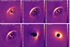 |
Fig. A.1 Reduction of Ks-band proto-planetary disc using our star-hopping RDI pipleine. These fainter discs were not recovered by Ren et al. (2023). |
In simple terms, we made simulated discs of different contrasts from the RMS map of the ‘scaled reference’ image. Here we discuss the detailed step-by-step explanation for generating the simulated disc and estimating the error maps:
Scaled Reference Images (sref): Each sref image, generated during the LOCI reduction, serves as the best reference for corresponding science images.
Difference Image Map (dimg): We subtract the median of the sref images from each individual sref image to create a difference image map. This is calculated as dimgi = srefi -median(sref).
Derotation: To ensure sufficient derotation, we derotate each dimgi image by an angle of i × 0.1 degrees. We do not use the real derotation for the dataset, as these would recover the real planets and possibly other astrophysical signal.
RMS Map Construction: The RMS map was constructed from the median combination of the dimg images. To be successfully detected, simulated signal has to be inserted above the noise level defined by this RMS map.
Simulated Disc Creation: Using the RMS map, we create a disc with an inner radius of 10 pixels and an outer radius of 80 pixels. This disc is then scaled in intensity and inserted into the science image to simulate proto-planetary discs.
Disc Recovery and Error Analysis: We use the HR8799+simulated disc system as an input for our pipeline and recover the simulated disc. In order to evaluate the precision of disc recovery, we calculate fractional error maps using the following equation:
 (B.1)
(B.1)Repetition and Scaling: We repeat the entire process multiple times, scaling the RMS map by a set of multiplicative factors (n = 1, 3, 5, 7, 10, 20, 30, 40, 50, 75, and 100) to assess the impact of varying disc brightness on the recovery fraction.
Once we have the recovery maps for different contrast levels of the inserted disc, we use them to construct random and systematic error maps. The recovery map is divided into sub-annuli of 4 pixels, and the mean (which represents the systematic error) and standard deviation (which represents the random error) of pixel counts in each annulus are computed. Figure B.1 shows the radial profiles of the simulated disc (inserted with 30σ brightness) alongside the corresponding profile recovered using the star-hopping pipeline. We find that there is no significant flux loss or morphology change in the disc. We also observe that both the systematic and random error decrease with increasing radial separation as shown in Figures B.2 and B.3.
Furthermore, we find that both the random and systematic error decrease as the brightness of the disc increases. Figures B.4 and B.5 show this trend for a region between 20 and 30 pixels. Thus, for a high S/N dataset like that of LkCa 15 in this work (> 150 σ), the error bars are on the order of ≤ 4% for the disc.
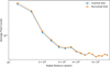 |
Fig. B.1 Comparison of the radial profile of the simulated (blue) and recovered disc (orange) images at 30 σ brightness level. |
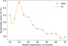 |
Fig. B.2 Systematic error map for a disc of brightness 30 σ. |
 |
Fig. B.3 Random error map for a disc of brightness 30 σ. |
Appendix C Qφ and Uφ images
Polarimetric pipelines like IRDAP produce azimuthal Stokes frames Qφ and Uφ by rotating the Q/U maps such that Qφ captures polarisation perpendicular (or parallel) to the radial direction and Uφ captures the 45°-offset component (de Boer et al. 2020). While Qφ often exhibits higher signal to noise because it concentrates azimuthal disc signal into one frame, both Qφ and Uφ together retain exactly the same information as the original Q/U pair (no Stokes information is lost by this basis rotation). However, for inclined and flared discs, multiple scattering and three dimensional surface geometry can introduce genuine non azimuthal polarisation manifest as astrophysical signal in Uφ and even negative Qφ values up to several percent of the total polarised flux (e.g. up to ~ 4.5% in generic MCFOST models at i = 40°) (Canovas et al. 2015). These non-azimuthal signatures are washed out if one examines Qφ alone, potentially biasing inferences of flaring or disc asymmetry.
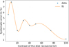 |
Fig. B.4 Systematic error map as a function of disc brightness calculated in the annular region of 20 to 30 pixels from the central star. |
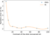 |
Fig. B.5 Random error map as a function of disc brightness, calculated within the annular region spanning 20 to 30 pixels from the central star. |
In contrast, the Stokes Q and U images preserve the full polarisation vector at each pixel, allowing direct pixel by pixel comparison to RADMC-3D’s synthetic Q and U outputs without ambiguity from an assumed azimuthal pattern. Therefore, we chose to focus on modelling the Q and U images, as they more effectively represent the disc’s geometry. For completeness, the Qφ and Uφ images are shown in Figure C.1.
Appendix D Calculations of 
To obtain the best-fit solution, we need to compute the mean of the reduced chi-square ( ) for our images. The (
 ) in turn consists of both the mean image reduced chi-square (
 ) and the mean flux chi-square (
 ) which can also be expressed as,
 (D.1)
(D.1)
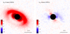 |
Fig. C.1 The Qφ and Uφ images are produced by the IRDAP pipeline, as described by van Holstein et al. (2020). |
To calculate  , we first calculate the image chi-square (
 ) in the region (rgn) from 10 to 75 pixels, considering the pixels with counts above 2 times the standard deviation in the background region (2σ). The σ is determined by calculating the robust sigma in the background region between 75 to 100 pixels. In the above equation D.1, the model images are scaled before computing the
  . Thus the
  is given as,
 (D.2)
(D.2)
where, the nsig is the number of effective data-points in the rgn. The nsig is obtained by dividing the total number of pixels in the rgn with counts greater than 2σdata by the resolution area of each pixel and tp is the total number of pixels in the rgn. In the above calculation, the model images are scaled before calculating  . The scaling factor is determined by minimising the standard deviation of the residuals between the observed and modeled data within a selected region (10 to 70 pixels). The scaled model is then computed by multiplying the initial model image by the scaling factor. Now, to get the
  , we need to divide
  by nsig for all our images as given by,
 (D.3)
(D.3)
In order to measure the total flux mismatch, for each image the  is calculated as,
 (D.4)
(D.4)
where the uncertainties in science fluxes are taken to be around 15% for NIR and 10% for ALMA, fdata and fmodel are the total data and model fluxes in the rgn. Since the polarimetric images contain both positive and negative fluxes, we needed to use the absolute values of the fluxes to calculate the  for the Q and U images. Thus our final chi-square (
 ) which we used for the minimisation can be expanded as,
 (D.5)
(D.5)
Summary of χ2 parameters and the flux differences (in ~%) for the olivine and CAHP grain models.
where the subscript R and f represent the reduced and flux chisquares and the I, Q, U, 880, and 1300 represent the I, Q, and U images in the Ks-band, while 880 and 1300 represent the ALMA images in 880μm and 1300μm.
To obtain the best-fit model, we begin with the initial parameters from the literature (Jin et al. 2019; Swastik et al. 2021) and used the Basin-hopping minimisation algorithm from the Scipy.optimise4 Python package, minimising the  calculated in equation D.5 to derive the optimal solution for our data. Due to the computational demands of the minimisation search process in RADMC-3D, it takes approximately 8 hours to complete approximately 500 iterations, making it impractical to find an exact best-fit solution for the data within these constraints. Instead, the solution obtained after 10000 iterations represents the closest approximation achievable. The
  and other minimisation parameter results are listed in Table D.1.
All Tables
Summary of χ2 parameters and the flux differences (in ~%) for the olivine and CAHP grain models.
All Figures
|
Fig. 1 Left to right: IRDIS total intensity K-band, Stokes Q - K-band, and Stokes U - K-band images observed from VLT-SPHERE. |
| In the text | |
|
Fig. 2 Inverted K-band polarisation fraction ( |
| In the text | |
|
Fig. 3 Schematic diagram showing the axis orientation for the E field chosen in this paper. The +Q is aligned in the X direction and -Q is aligned in the Y direction. The blue points represent the dust grains, while the arrows indicate the scattered photons towards the observer, an incomparably large distance away. |
| In the text | |
|
Fig. 4 Signs of Stokes parameters taken in this paper indicating the positive and negative regions in Q and U images. |
| In the text | |
|
Fig. 5 Comparison of RADMC-3D model with olivine grains and observed data. The sequence from left to right shows the data, the simulated model, and the residuals. The top row is the K-band total intensity image, followed by the K-band Stokes Q, and the Stokes U. The fourth and fifth rows at the bottom correspond to ALMA 880 μm and 1300 μm images, respectively. |
| In the text | |
|
Fig. 6 Schematic diagram of our LkCa 15 proto-planetary disc with olivine grains. The black and orange represent the micron- and millimetre-sized grains, respectively. |
| In the text | |
|
Fig. 7 Comparison of the SPHERE Ks-band scattered light phase function (red points) to a family of CAHP aggregate grain models with monomer counts 16, 32,..., 1024 (solid coloured lines), and to a compact ~ 8 μm olivine grain (dashed pink). Top : normalised scattered-light intensity (flux) as a function of scattering angle. Bottom : polarised phase function versus scattering angle for the same model series and data points. |
| In the text | |
|
Fig. 8 Side by side comparison between the observations and a RADMC-3D model with CAHP-128-100nm grains, plus residuals. Left to right: data, model, residuals. Rows (top to bottom): K-band total intensity, Stokes Q, and Stokes U. We did not model the ALMA images using CAHP grains as we do not have the optical properties of the CAHP grains at millimetre wavelengths. |
| In the text | |
|
Fig. 9 Polarisation fraction as a function of scattering angle for the LkCa 15 disc. Red points: SPHERE Ks-band data (debiased). Blue: CAHP-128-100 nm high-porosity aggregate model. Dashed black: Rayleigh limit. The broad, sub-Rayleigh peak indicates that scattering is dominated by porous aggregate grains rather than compact Mie spheres. |
| In the text | |
|
Fig. 10 Left : IRDIS K-band reduction with LOCI algorithm after removing most of the disc in order to detect obscured planets and to estimate the contrast limit as shown in Figure 11. |
| In the text | |
|
Fig. 11 5σ contrast curve in the K band obtained by removing the LkCa 15 proto-planetary disc. The dashed red line represents the detection limit at the brightest part of the discs. The mass estimates for the companions were obtained using DUSTY models assuming the stellar age to be 1 Myr for LkCa 15. |
| In the text | |
|
Fig. 12 Figure illustrates the model-estimated relative abundances of three grain sizes, compared to those predicted by the power law by Dohnanyi (1969). The data pairs were generated a Monte Carlo simulation with an asymmetric Gaussian distribution (see Section 4 for more details). |
| In the text | |
|
Fig. A.1 Reduction of Ks-band proto-planetary disc using our star-hopping RDI pipleine. These fainter discs were not recovered by Ren et al. (2023). |
| In the text | |
|
Fig. B.1 Comparison of the radial profile of the simulated (blue) and recovered disc (orange) images at 30 σ brightness level. |
| In the text | |
|
Fig. B.2 Systematic error map for a disc of brightness 30 σ. |
| In the text | |
|
Fig. B.3 Random error map for a disc of brightness 30 σ. |
| In the text | |
|
Fig. B.4 Systematic error map as a function of disc brightness calculated in the annular region of 20 to 30 pixels from the central star. |
| In the text | |
|
Fig. B.5 Random error map as a function of disc brightness, calculated within the annular region spanning 20 to 30 pixels from the central star. |
| In the text | |
|
Fig. C.1 The Qφ and Uφ images are produced by the IRDAP pipeline, as described by van Holstein et al. (2020). |
| In the text | |
Current usage metrics show cumulative count of Article Views (full-text article views including HTML views, PDF and ePub downloads, according to the available data) and Abstracts Views on Vision4Press platform.
Data correspond to usage on the plateform after 2015. The current usage metrics is available 48-96 hours after online publication and is updated daily on week days.
Initial download of the metrics may take a while.