© The Authors 2026

1. Introduction

The Faraday rotation effect is one of the most well-known effects in magnetized plasmas. This phenomenon describes the rotation of the plane of polarization of linearly polarized electromagnetic waves propagating along a background magnetic field in a multicomponent plasma (Chen 1984). This is easily understood: any linearly polarized wave can be decomposed into right- and left-handed circularly polarized waves, each propagating at a different speed along the magnetic field. The phase difference between these circularly polarized waves gives rise to Faraday rotation. In a magnetized ion-electron plasma (Krall & Trivelpiece 1973), the rotation angle is related to the plasma density, the magnitude of the background magnetic field, and the distance to the source of the electromagnetic radiation. A similar analysis has been extended to ion-electron-positron plasmas (Park & Blackman 2010). Therefore, the Faraday rotation effect can be helpful as a tool for estimating plasma properties.

In most plasmas, the Faraday rotation is complex to measure (Chen 1984). However, it has been used extensively in astrophysics (Kulsrud 2005), where interstellar paths are long and magnetic fields are strong enough to have a good estimation of the plasma densities near pulsars, or in the formation of new stars (Chen 1984; Kulsrud 2005). Furthermore, Faraday rotations have been used to obtain the magnetic field in active galactic nuclei (Asada et al. 2002; Attridge et al. 2005), pulsars and quasars (Han et al. 2006; Asada et al. 2002; Zavala & Taylor 2005), the interstellar medium (Xu et al. 2005; Dreher et al. 1987; Pshirkov et al. 2011; Gaensler et al. 2005; Simard-Normandin et al. 1981; Murgia et al. 2004), and the cosmic microwave background (Campanelli et al. 2004; Kosowsky & Loeb 1996).

In this spirit, one may wonder whether Faraday rotation could be used to extract information on not only plasma properties but also the curvature of space-time or black hole masses. The answer is affirmative, and this has been extensively studied in the context of gravitational Faraday rotation (GFR). The GFR effect occurs when the plane of polarization of photons (that follow null geodesics) rotates in stationary space-times. This has been investigated for Kerr black holes and accretion disks (Connors & Stark 1977; Connors et al. 1980; Dehnen 1973; Tamburini et al. 2011; Broderick & Blandford 2003; Chandrasekhar 1983; Ishihara et al. 1988; Sereno 2004; Nouri-Zonoz 1999), with the effect of space-time rotation being shown in the parallel transport of the light polarization vector. Considering these works, we study a different aspect of Faraday rotation on electromagnetic waves, including magnetized plasma, in this manuscript. Hence, we study the propagation of circularly polarized electromagnetic waves in magnetized plasmas in the curved space-time far a Schwarzschild black hole. This problem differs from the works mentioned above about GFR for several reasons. In particular, depending on Killing observers, GRF does not appear in the Schwarzschild (static) metric. Also, light does not follow null geodesics in a plasma, since the velocity of an electromagnetic wave in a plasma is not the speed of light in a vacuum, as the dispersion relation of electromagnetic waves must now account for the oscillation frequency of the charged particles. Therefore, it is interesting to investigate what other contributions to Faraday rotation can be introduced by a magnetized plasma in the curved space-time created by a Schwarzschild black hole.

Specifically, we show that the phase difference between two circularly polarized electromagnetic waves (left and right) encodes information about space-time curvature. The waves propagate in a magnetized plasma that is restricted from moving along the radial direction defined by the black hole, i.e., we assume that there is no stellar wind. This condition is considered as it produces an exact solution to the problem. Physically, a plasma can behave this way far from the black hole, so its angular velocity is larger than any radial velocity. Thus, we show that the magnetically induced Faraday rotation of the electromagnetic waves in these plasmas now relates the Faraday rotation angle to the plasma densities, the magnitude of a radial magnetic field, the distance to the black hole, and its mass. In this way, the rotation of the plane of polarization of electromagnetic waves in a plasma can be used as a tool to estimate not only the plasma properties, but also the other characteristics of astrophysical compact objects through the measurement of this specific interaction between plasmas and the electromagnetic fields around or near those astrophysical bodies.

2. Plasmas in the vicinity of a Schwarzschild black hole

Plasmas in curved space-times can be described by covariant fluid dynamical equations. These are the conservation laws derived from Einstein’s equations. However, in this work, we assume that the plasma does not gravitate. This means that its energy-momentum tensor does not contribute significantly to the Einstein equations. Thus, the dynamics can be described simply as a plasma moving in a given background metric of the space-time, and the presence of the plasma does not alter that space-time. The restrictions imposed by this diluted plasma approximation will be analyzed in a future manuscript. However, this approximation implies that the energy density of the electromagnetic field is much less than the effective energy density associated with a black hole; namely, E² + B² ≪ c⁸/(G³M²) (Frolov & Koek 2024). This condition is certainly fulfilled far from the black, where the electric (and magnetic) field solution decays as 1/r (see Sect. 3.2).

Major insights are gained if the covariant dynamics of plasma around black holes are described in terms of the 3 + 1 formulation of general relativity. This analysis has been carried out in Buzzi et al. (1995), Thorne et al. (1986), and here we only display its main results. A fiducial observer (FIDO) is used to define the physical quantities. This FIDO is defined as the one at rest with respect to the black hole (Thorne et al. 1986), using a local three-dimensional Cartesian system defined by the orthonormal basis of vectors of unit length ${\mathbf{e}}_{\widehat{r}}=\alpha {\partial }_r$, ${\mathbf{e}}_{\widehat{\theta }}=r^{-1}{\partial }_{\theta }$, and ${\mathbf{e}}_{\widehat{\varphi }}={(rsin\theta )}^{-1}{\partial }_{\varphi }$, where α is the lapse function. For the Schwarzschild metric, it is given by

$$\begin{array}{c}\hfill \alpha (r)={(1-\frac{2M}{r})}^{1/2},\end{array}$$(1)

where M is the black hole mass, and r is the radial coordinate. This basis has the vector algebra ${\mathbf{e}}_{\widehat{a}}·{\mathbf{e}}_{\widehat{b}}={\delta }_{\mathit{ab}}$ and ${\mathbf{e}}_{\widehat{a}}\times {\mathbf{e}}_{\widehat{b}}={ϵ}_{\mathit{abc}}{\mathbf{e}}_{\widehat{c}}$, where ϵ_abc is the completely antisymmetric symbol (Thorne et al. 1986). This basis of three-dimensional vectors defines a one-form dual basis ${\mathit{w}}^{\widehat{r}}={\alpha }^{-1}dr$, ${\mathit{w}}^{\widehat{\theta }}=rd\theta$ and ${\mathit{w}}^{\widehat{\varphi }}=rsin\theta d\varphi$, such that ${\mathit{w}}^{\widehat{a}}{\mathbf{e}}_{\widehat{b}}={{\delta }^a}_b$. Therefore, any such three-dimensional vector has the form $\mathbf{Y}=Y^{\widehat{a}}{\mathbf{e}}_{\widehat{a}}$ (Thorne et al. 1986). This is equivalent to defining vectors using a 3 + 1 decomposition by projecting every tensor onto time-like and space-like hypersurfaces. For this, we defined the three-metric γ_μν of the spacelike hypersurfaces of the metric g_μν. Also, we used a normalized timelike vector field, n^μ, obeying n_μn^μ = −1 and n_μγ^μν = 0. Thus, the metric was written as g_μν = γ_μν − n_μn_ν, and the timelike vector was constructed in terms of the lapse function as n_μ = (α, 0, 0, 0). For example, using the electromagnetic field tensor F_μν, we can define the spacelike electric and magnetic vector fields as E^μ = n_νF^νμ and B^μ = n_ρϵ^ρμαβF_αβ/2 (Asenjo et al. 2013), respectively, where ϵ^ρμαβ is the totally antisymmetric tensor.

With all this, for the Schwarzschild metric, Maxwell equations can be written for the electric and magnetic field by projecting the equation ∇_νF^μν = 4πJ^μ onto the time-like and space-like hypersurfaces (where J^μ is the plasma four-current vector that satisfies a conservation equation, ∇_μJ^μ = 0). Thus, they become (Thorne et al. 1986; Asenjo et al. 2013)

$$\begin{array}{cc}\hfill \mathrm{\nabla }·\mathbf{B}& =0,\hfill \end{array}$$(2)

$$\begin{array}{cc}\hfill \mathrm{\nabla }·\mathbf{E}& =4\pi \rho \hfill \end{array}$$(3)

$$\begin{array}{cc}\hfill \frac{\partial \mathbf{B}}{\partial t}& =-\mathrm{\nabla }\times \left(\alpha \mathbf{E}\right),\hfill \end{array}$$(4)

$$\begin{array}{cc}\hfill \frac{\partial \mathbf{E}}{\partial t}& =\mathrm{\nabla }\times \left(\alpha \mathbf{B}\right)-4\pi \alpha \mathbf{J},\hfill \end{array}$$(5)

where E and B are the electric and magnetic fields measured by a FIDO, respectively. Here, the coordinate t corresponds to the universal time defined in the metric, different from the proper time, τ, of the plasma constituents, whose relation is dτ/dt = α (Thorne et al. 1986). Also, the ∇ operator was calculated in the three-dimensional foliation of space-time, i.e., it is the spatial covariant derivative derived from γ_μν (Buzzi et al. 1995; Thorne et al. 1986; Asenjo et al. 2013). For example, the ∇⋅ and ∇× operators must be calculated by the corresponding operations on the curvilinear spatial coordinates defined by γ_μν. The charge density and current vector density measured by the FIDO are obtained using the same 3+1 decomposition procedure. They are defined as ρ = n_μJ^μ, and Jⁱ = γⁱ_μJ^μ, such that

$$\begin{array}{c}\hfill \rho ={\displaystyle \sum _s}{q}_s{\gamma }_s{n}_s,\mathbf{J}={\displaystyle \sum _s}{q}_s{\gamma }_s{n}_s{\mathbf{v}}_s,\end{array}$$(6)

with the s index representing the different plasma species; thus, q_s, n_s, and v_s are the charge, number density, and velocity of the corresponding species, s. Also ${\gamma }_s={(1-{\mathbf{v}}_s·{\mathbf{v}}_s)}^{-1/2}$. We have chosen units so that the speed of light, c, and the gravitational constant, G, are both equal to 1.

In this 3 + 1 formalism, the plasma dynamics for each species can also be put in a three-dimensional vectorial fashion, or by using the above orthonormal basis, or through hypersurfaces projections, on the continuity equation and the energy-momentum conservation equation (Buzzi et al. 1995). The continuity equation ∇_μJ^μ = 0 becomes (Thorne et al. 1986; Buzzi et al. 1995)

$$\begin{array}{c}\hfill \frac{\partial }{\partial t}\left({\gamma }_s{n}_s\right)+\mathrm{\nabla }·\left(\alpha {\gamma }_s{n}_s{\mathbf{v}}_s\right)=0.\end{array}$$(7)

From the conservation law, ∇_νT_s^μν = 0, of the energy-momentum tensor for each species, T_s^μν = Λ_sU_s^μU_s^ν + P_sg^μν, we can obtain the energy and the momentum conservation equations. Here, each species fluid velocity, U_s^μ = (γ_s, γ_sv_s), P_s is the pressure of each fluid representing the particles with mass m_s, and Λ_s is given by

$$\begin{array}{c}\hfill {\mathrm{\Lambda }}_s={\epsilon }_s+P_s=m_s{n}_s+\left(\frac{{\mathrm{\Gamma }}_s}{{\mathrm{\Gamma }}_s-1}\right)P_s,\end{array}$$(8)

with ε_s = m_sn_s + P_s/(Γ_s − 1) the energy density, and Γ_s the polytropic index for each species (Buzzi et al. 1995). For instance, if the temperature, T, tends to infinity (T → ∞), then Γ_s → 4/3. On the contrary, if T → 0, then Γ_s → 5/3. Besides, we chose the equation of state P_s = β_sn_s^Γ_s in order to preserve the specific entropy (given that β_s is constant). Thus, the energy conservation equation is (Buzzi et al. 1995)

$$\begin{array}{cc}& \frac{1}{\alpha }\frac{\partial P_s}{\partial t}-\frac{1}{\alpha }\frac{\partial }{\partial t}\left({\gamma }_s^2{\mathrm{\Lambda }}_s\right)-\mathrm{\nabla }·\left({\gamma }_s^2{\mathrm{\Lambda }}_s{\mathbf{v}}_s\right)\hfill \\ \hfill & +2{\gamma }_s^2{\mathrm{\Lambda }}_s\mathbf{a}·{\mathbf{v}}_s+{\gamma }_s{q}_s{n}_s(\mathbf{E}·{\mathbf{v}}_s)=0,\hfill \end{array}$$(9)

with a the gravitational acceleration experienced by the FIDO (Thorne et al. 1986; Buzzi et al. 1995)

$$\begin{array}{c}\hfill \mathbf{a}=-\mathrm{\nabla }ln\alpha =a{\mathbf{e}}_{\widehat{r}},\end{array}$$(10)

where a = −M/(αr²) is the magnitude of the acceleration. Finally, the momentum conservation equation becomes (Buzzi et al. 1995)

$$\begin{array}{cc}& {\gamma }_s^2{\mathrm{\Lambda }}_s{D}_{\tau }{\mathbf{v}}_s={\gamma }_s{q}_s{n}_s(\mathbf{E}+{\mathbf{v}}_s\times \mathbf{B})-\mathrm{\nabla }{P}_s\hfill \\ \hfill & -{\mathbf{v}}_s({\gamma }_s{q}_s{n}_s\mathbf{E}·{\mathbf{v}}_s+\frac{1}{\alpha }\frac{\partial P_s}{\partial t})\hfill \\ \hfill & -{\gamma }_s^2{\mathrm{\Lambda }}_s({\mathbf{v}}_s({\mathbf{v}}_s·\mathbf{a})-\mathbf{a}),\hfill \end{array}$$(11)

where $D_{\tau }\equiv (1/\alpha ){\partial }_t+{\mathbf{v}}_s·\mathrm{\nabla }$ is the effective convective derivative.

The previous set of equations describes the general theory for plasmas in a static space-time. However, to better understand plasma dynamics, let us write the previous equations in a more explicit form using general spherical coordinates. We assume that every physical quantity depends only on the radial direction in order to study plasma waves propagating in a radially outward direction in the following sections. In particular, the radial propagation assumption for electromagnetic waves allows us to consider light moving without experiencing a bend in its trajectory due to the black hole gravity (Plebanski 1960; Parker 1969). Light only experiences redshift and Faraday rotation in this case due to the magnetized plasma.

Due to the spherical symmetry and without loss of generality, we chose the θ = π/2 plane to describe the dynamics of the plasma quantities measured by the FIDO. The constraint (2) becomes simply

$$\begin{array}{c}\hfill \frac{\alpha }{r^2}\frac{\partial }{\partial r}\left(r^2{B}^{\widehat{r}}\right)=0,\end{array}$$(12)

while the components of Eq. (4) read

$$\begin{array}{cc}\hfill \frac{\partial B^{\widehat{r}}}{\partial t}& =0,\hfill \end{array}$$(13)

$$\begin{array}{cc}\hfill \frac{\partial B^{\widehat{\theta }}}{\partial t}& =\frac{\alpha }{r}\frac{\partial }{\partial r}\left(\alpha r{E}^{\widehat{\varphi }}\right),\hfill \end{array}$$(14)

$$\begin{array}{cc}\hfill \frac{\partial B^{\widehat{\varphi }}}{\partial t}& =-\frac{\alpha }{r}\frac{\partial }{\partial r}\left(\alpha r{E}^{\widehat{\theta }}\right).\hfill \end{array}$$(15)

These equations imply (Buzzi et al. 1995)

$$\begin{array}{cc}\hfill B^{\widehat{r}}& =\frac{{\lambda }_0}{r^2},\hfill \end{array}$$(16)

$$\begin{array}{cc}\hfill \frac{\partial B_{\pm }}{\partial t}& =\mp \frac{i\alpha }{r}\frac{\partial }{\partial r}\left(\alpha r{E}_{\pm }\right),\hfill \end{array}$$(17)

where λ₀ is an arbitrary constant, and we have defined $B_{\pm }=B^{\widehat{\theta }}\pm i{B}^{\widehat{\varphi }}$ and $E_{\pm }=E^{\widehat{\theta }}\pm i{E}^{\widehat{\varphi }}$. Thus, the ± sign stands for both polarizations of the wave.

On the other hand, Eq. (3) is

$$\begin{array}{c}\hfill \frac{\alpha }{r^2}\frac{\partial }{\partial r}\left(r^2{E}^{\widehat{r}}\right)=4\pi {\displaystyle \sum _s}{\gamma }_s{q}_s{n}_s,\end{array}$$(18)

and the components of Eq. (5) are

$$\begin{array}{cc}\hfill \frac{\partial E^{\widehat{r}}}{\partial t}& =-4\pi \alpha {\displaystyle \sum _s}{\gamma }_s{q}_s{n}_s{u}_s,\hfill \end{array}$$(19)

$$\begin{array}{cc}\hfill \frac{\partial E^{\widehat{\theta }}}{\partial t}& =-\frac{\alpha }{r}\frac{\partial }{\partial r}\left(\alpha r{B}^{\widehat{\varphi }}\right)-4\pi \alpha {\displaystyle \sum _s}{\gamma }_s{q}_s{n}_s{v}_s^{\widehat{\theta }},\hfill \end{array}$$(20)

$$\begin{array}{cc}\hfill \frac{\partial E^{\widehat{\varphi }}}{\partial t}& =\frac{\alpha }{r}\frac{\partial }{\partial r}\left(\alpha r{B}^{\widehat{\theta }}\right)-4\pi \alpha {\displaystyle \sum _s}{\gamma }_s{q}_s{n}_s{v}_s^{\widehat{\varphi }},\hfill \end{array}$$(21)

where $u_s=v_s^{\widehat{r}}$ is the radial component of the fluid velocity. The previous equations imply that

$$\begin{array}{c}\hfill \frac{\partial E_{\pm }}{\partial t}=\pm \frac{i\alpha }{r}\frac{\partial }{\partial r}\left(\alpha r{B}_{\pm }\right)-4\pi \alpha {\displaystyle \sum _s}{\gamma }_s{q}_s{n}_s{v}_{\pm s},\end{array}$$(22)

where $v_{s\pm }=v_s^{\widehat{\theta }}\pm i{v}_s^{\widehat{\varphi }}$. In this way, Eqs. (17) and (22) can be combined to produce

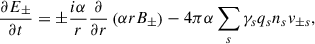
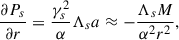
$$\begin{array}{c}\hfill \frac{{\partial }^2{E}_{\pm }}{\partial t^2}=\frac{\alpha }{r}\frac{\partial }{\partial r}\left[{\alpha }^2\frac{\partial }{\partial r}\left(r\alpha E_{\pm }\right)\right]-4\pi \alpha {\displaystyle \sum _s}{q}_s\frac{\partial }{\partial t}\left({\gamma }_s{n}_s{v}_{\pm s}\right).\end{array}$$(23)

Similarly, for the plasma dynamics, the continuity equation, Eq. (7), becomes

$$\begin{array}{c}\hfill \frac{\partial }{\partial t}\left({\gamma }_s{n}_s\right)+\frac{\alpha }{r^2}\frac{\partial }{\partial r}\left(r^2\alpha {\gamma }_s{n}_s{u}_s\right)=0,\end{array}$$(24)

while the energy conservation equation, Eq. (9), is now

$$\begin{array}{cc}& \frac{1}{\alpha }\frac{\partial P_s}{\partial t}-\frac{1}{\alpha }\frac{\partial }{\partial t}\left({\gamma }_s^2{\mathrm{\Lambda }}_s\right)-\frac{\alpha }{r^2}\frac{\partial }{\partial r}\left({\gamma }_s^2{\mathrm{\Lambda }}_s{u}_s\right)\hfill \\ \hfill & +{\gamma }_s{q}_s{n}_s\mathbf{E}·{\mathbf{v}}_{\mathbf{s}}+2{\gamma }_s^2{\mathrm{\Lambda }}_{s}a{u}_s=0.\hfill \end{array}$$(25)

In this notation, $\mathbf{E}·{\mathbf{v}}_{\mathbf{s}}=E_{\pm }·v_{s,\pm }^{\ast }+E_{\widehat{r}}{u}_s$.

Finally, the components of the momentum equation, Eq. (11), are, respectively,

$$\begin{array}{cc}& {\gamma }_s^2{\mathrm{\Lambda }}_s{D}_{\tau }{u}_s+\alpha \frac{\partial P_s}{\partial r}-{\gamma }_s{q}_s{n}_s(E^{\widehat{r}}+v_s^{\widehat{\theta }}{B}^{\widehat{\varphi }}-v_s^{\widehat{\varphi }}{B}^{\widehat{\theta }})\hfill \\ \hfill & +u_s({\gamma }_s{q}_s{n}_s\mathbf{E}·{\mathbf{v}}_{\mathbf{s}}+\frac{1}{\alpha }\frac{\partial P_s}{\partial t})+{\gamma }_s^2{\mathrm{\Lambda }}_s(u_s^2-1)a=0,\hfill \end{array}$$(26)

$$\begin{array}{cc}& {\gamma }_s^2{\mathrm{\Lambda }}_s{D}_{\tau }{v}_s^{\widehat{\theta }}-{\gamma }_s{q}_s{n}_s(E^{\widehat{\theta }}-u_s{B}^{\widehat{\varphi }}+v_s^{\widehat{\varphi }}{B}^{\widehat{r}})\hfill \\ \hfill & +v_s^{\widehat{\theta }}({\gamma }_s{q}_s{n}_s\mathbf{E}·{\mathbf{v}}_{\mathbf{s}}+\frac{1}{\alpha }\frac{\partial P_s}{\partial t})+{\gamma }_s^2{\mathrm{\Lambda }}_s{v}_s^{\widehat{\theta }}{u}_{s}a=0,\hfill \end{array}$$(27)

$$\begin{array}{cc}& {\gamma }_s^2{\mathrm{\Lambda }}_s{D}_{\tau }{v}_s^{\widehat{\varphi }}-{\gamma }_s{q}_s{n}_s(E^{\widehat{\varphi }}+u_s{B}^{\widehat{\theta }}-v_s^{\widehat{\theta }}{B}^{\widehat{r}})\hfill \\ \hfill & +v_s^{\widehat{\varphi }}({\gamma }_s{q}_s{n}_s\mathbf{E}·{\mathbf{v}}_{\mathbf{s}}+\frac{1}{\alpha }\frac{\partial P_s}{\partial t})+{\gamma }_s^2{\mathrm{\Lambda }}_s{v}_s^{\widehat{\varphi }}{u}_{s}a=0.\hfill \end{array}$$(28)

3. Circularly polarized waves

The system studied in the previous section is suitable for investigating right- and left-handed circularly polarized wave propagation in a magnetized plasma at a given radial distance from the black hole. This plasma is immersed in a background magnetic field along the radial direction. This magnetic field can be found as the solution of Eq. (16) demanding λ₀ = B₀ l², where l is some characteristic scale length of this field to be determined by the dynamics of the system, or equivalently, a particular radius at which B₀ is known. Thus, electromagnetic waves can propagate along this radial magnetic field and, depending on the properties of the plasma, a far observer can measure the right- or left-handed polarized components, thereby determining their phase difference.

As the plasma is assumed not to move radially (no stellar wind),

$$\begin{array}{c}\hfill u_s=0,\end{array}$$(29)

which allows us to find an exact solution to the plasma equations. This situation can occur for a plasma far from the black hole (see following Sect. 5). The validity of the condition given by Eq. (29) for the obtained solution is discussed in Sect. 7.

Also, let us consider that the plasma thermodynamic properties are stationary, namely,

$$\begin{array}{c}\hfill \frac{\partial n_s}{\partial t}=0,\frac{\partial P_s}{\partial t}=0,\frac{\partial {\mathrm{\Lambda }}_s}{\partial t}=0.\end{array}$$(30)

We can make the ansatz

$$\begin{array}{c}\hfill \frac{\partial {\gamma }_s}{\partial t}=0,\end{array}$$(31)

which will be confirmed below, as it will naturally appear as a direct consequence of a circularly polarized wave propagating in relativistic magnetized plasmas (Asenjo et al. 2009).

Lastly, although the above system is general for plasmas that could not be quasi-neutral, for the time and space scales under consideration in this work, we assume the quasi-neutral approximation

$$\begin{array}{c}\hfill {\displaystyle \sum _s}{\gamma }_s{q}_s{n}_s=0.\end{array}$$(32)

From Eq. (18) we can consider a solution with $E_{\widehat{r}}=0$, which is consistent with Eq. (19). Also, note that the continuity equation is exactly satisfied.

Conditions (29)–(32) allow us to find the exact dynamics for circularly polarized electromagnetic waves along a background magnetic field in a homogeneous relativistic electron-positron plasma. In the following, we show how the system can be solved in the mildly relativistic quasi-monochromatic approximation, considering the radial dynamics of the electromagnetic plasma wave induced by the space-time curvature. This is different from what was done, for instance, in Buzzi et al. (1995) and Sakai & Kawata (1980), in which the complete Eikonal approximation was used to solve electromagnetic propagation.

3.1. Exact dynamics

Owing to our assumptions, Eq. (25) simply predicts

$$\begin{array}{c}\hfill \mathbf{E}·{\mathbf{v}}_s=0,\end{array}$$(33)

while the radial component of the momentum equation, Eq. (26), allows us to calculate the pressure condition for the radial equilibrium of the plasma,

$$\begin{array}{c}\hfill \alpha \frac{\partial P_s}{\partial r}-{\gamma }_s{q}_s{n}_s(v_s^{\widehat{\theta }}{B}^{\widehat{\varphi }}-v_s^{\widehat{\varphi }}{B}^{\widehat{\theta }})-{\gamma }_s^2{\mathrm{\Lambda }}_{s}a=0.\end{array}$$(34)

Manipulating the other components of the momentum equation can provide us with more insight into this propagation. For example, Eqs. (27) and (28) can be combined to give

$$\begin{array}{c}\hfill {\gamma }_s^2{\mathrm{\Lambda }}_s{D}_{\tau }{v}_{s\pm }={\gamma }_s{q}_s{n}_s(E_{\pm }\mp i{v}_{s\pm }{B}^{\widehat{r}}),\end{array}$$(35)

while Eqs. (27) and (28) yield

$$\begin{array}{c}\hfill {\gamma }_s^2{\mathrm{\Lambda }}_s(v_s^{\widehat{\theta }}{D}_{\tau }{v}_s^{\widehat{\theta }}+v_s^{\widehat{\varphi }}{D}_{\tau }{v}_s^{\widehat{\varphi }})=0,\end{array}$$(36)

where we have used E · v_s = 0. Given that v_s ⋅ ∇ = 0, the above condition can also be written as

$$\begin{array}{c}\hfill v_s^{\widehat{\theta }}{D}_{\tau }{v}_s^{\widehat{\theta }}+v_s^{\widehat{\varphi }}{D}_{\tau }{v}_s^{\widehat{\varphi }}=\frac{1}{2\alpha }\frac{\partial }{\partial t}[{\left(v_s^{\widehat{\theta }}\right)}^2+{\left(v_s^{\widehat{\varphi }}\right)}^2]=0,\end{array}$$(37)

implying that when E · v_s = 0, then ${(v_s^{\widehat{\theta }})}^2+{(v_s^{\widehat{\varphi }})}^2$ is constant in time. Therefore, our assumption about a constant gamma factor in time (Eq. (31)) is justified.

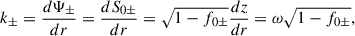
Now, we can use a temporal WKB (eikonal) wave approximation for the fields. In particular, we introduced a general temporal phase, with the wave frequency ω. Since ${(v_s^{\widehat{\theta }})}^2+{(v_s^{\widehat{\varphi }})}^2=(v_{s+}{v}_{s+}^{\ast }+v_{s-}{v}_{s-}^{\ast })/2$, then we can write

$$\begin{array}{c}\hfill v_{s\pm }(t,r)={\mathcal{V}}_{s\pm }(r)e^{i\omega t},\end{array}$$(38)

where the wave frequency, ω, must satisfy a dispersion relation, and ${\mathcal{V}}_{s\pm }(r)$ is a complex function, retaining the radial information of the wave propagation. Thus, the Lorentz factor becomes ${\gamma }_s={\gamma }_{s\pm }={(1-{\mathcal{V}}_{s\pm }{\mathcal{V}}_{s\pm }^{\ast })}^{-1/2}$, depending on the polarization of the wave.

Therefore, Eq. (35) can be readily written as

$$\begin{array}{c}\hfill (\frac{{\gamma }_{s\pm }{\mathrm{\Lambda }}_s\omega }{\alpha m_s{n}_s}\pm \frac{l^2}{r^2}{\mathrm{\Omega }}_{\mathit{cs}}){\mathcal{V}}_{s\pm }=-i\frac{q_s}{m_s}{\mathcal{E}}_{\pm },\end{array}$$(39)

where it must be noticed that $({\mathbf{v}}_s·\mathrm{\nabla }){\mathcal{V}}_{s\pm }\equiv 0$, and m_s is the mass of the constituents of each plasma fluid. Here, we can use the fact that the electric field has the same temporal wave phase, with the same frequency,

$$\begin{array}{c}\hfill E_{\pm }(t,r)={\mathcal{E}}_{\pm }(r)e^{i\omega t}.\end{array}$$(40)

Also, we have introduced the cyclotron frequency for each constituent,

$$\begin{array}{c}\hfill {\mathrm{\Omega }}_{\mathit{cs}}=\frac{q_s{B}_0}{m_s}.\end{array}$$(41)

The description of the dynamics is completed with Eq. (23), found through Maxwell’s equations, which is rewritten as

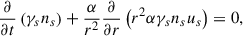
$$\begin{array}{c}\hfill 0={\omega }^2{\mathcal{E}}_{\pm }+\frac{\alpha }{r}\frac{\partial }{\partial r}\left[{\alpha }^2\frac{\partial }{\partial r}\left(r\alpha {\mathcal{E}}_{\pm }\right)\right]-4\pi i\omega \alpha {\displaystyle \sum _s}{q}_s{\gamma }_{s\pm }{n}_s{\mathcal{V}}_{s\pm }.\end{array}$$(42)

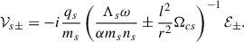
The complete system is now reduced to Eqs. (39) and (42). To solve it, it is necessary to find a solution for the velocity while the Lorentz factor fulfills the condition

$$\begin{array}{c}\hfill \sqrt{1-\frac{1}{{\gamma }_{s\pm }^2}}=\frac{\alpha V_{qs\pm }}{{\gamma }_{s\pm }\pm \alpha {\mathrm{\Theta }}_s},\end{array}$$(43)

where $V_{qs\pm }=(n_s/{\mathrm{\Lambda }}_s)(q_s{\mathcal{E}}_{\pm }/\omega )$ is a polarized quiver velocity perpendicular to the radial direction, and Θ_s = (m_sn_s/Λ_s)(Ω_csl²/ωr²) is the magnetization ratio of the plasma.

3.2. Mildly relativistic quasi-neutrality case

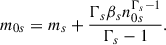
Equations (39), (42), and (43) can be solved numerically for ω and ${\mathcal{E}}_{\pm }$ (or ${\mathcal{V}}_{s\pm }$) by a shooting method with appropriate boundary conditions; for example, at r = l and r → ∞. This would depend of course on n_s(l), P_s(l), and B₀. As was previously suggested, it is expected that a measured Faraday rotation as a function of frequency would allow us to determine these plasma parameters and the black hole’s mass. Such analysis will be reported in future work. Although a complete solution is available, we resorted to an analytical approximation to gain an insight into the gravitationally induced Faraday rotation. Therefore, we now consider the mildly relativistic regime, in which γ_s± ≈ 1. This occurs when the quiver velocity, V_qs, is small compared to the speed of light. In this way, the solution for the velocity can be obtained directly from Eq. (39) as

$$\begin{array}{c}\hfill {\mathcal{V}}_{s\pm }=-i\frac{q_s}{m_s}{(\frac{{\mathrm{\Lambda }}_s\omega }{\alpha m_s{n}_s}\pm \frac{l^2}{r^2}{\mathrm{\Omega }}_{\mathit{cs}})}^{-1}{\mathcal{E}}_{\pm }.\end{array}$$(44)

By using Eq. (44) in Eq. (42), we finally obtain

$$\begin{array}{c}\hfill -({\omega }^2-\omega \alpha {\displaystyle \sum _s}{\omega }_{\mathit{ps}}^2{[\frac{{\mathrm{\Lambda }}_s\omega }{\alpha m_s{n}_s}\pm \frac{l^2}{r^2}{\mathrm{\Omega }}_{\mathit{cs}}]}^{-1}){\mathcal{E}}_{\pm }=\frac{\alpha }{r}\frac{\partial }{\partial r}\left[{\alpha }^2\frac{\partial }{\partial r}\left(r\alpha {\mathcal{E}}_{\pm }\right)\right],\end{array}$$(45)

where the plasma frequency for each species, ${\omega }_{\mathit{ps}}=\sqrt{4\pi q_s^2{n}_s/m_s}$, has been used explicitly. The above equation simplifies by using the new variable $D_{\pm }=\alpha r{\mathcal{E}}_{\pm }$, which leaves Eq. (45) as follows:

$$\begin{array}{c}\hfill 0={\alpha }^2\frac{{\partial }^2{D}_{\pm }}{\partial r^2}+\frac{2M}{r^2}\frac{\partial D_{\pm }}{\partial r}+(\frac{{\omega }^2}{{\alpha }^2}-{\displaystyle \sum _s}\frac{{\omega }_{\mathit{ps}}^2}{1+\frac{P_s}{m_s{n}_s}\left(\frac{{\mathrm{\Gamma }}_s}{{\mathrm{\Gamma }}_s-1}\right)\pm \frac{\alpha l^2{\mathrm{\Omega }}_{\mathit{cs}}}{\omega r^2}})D_{\pm }.\end{array}$$(46)

This equation depends on each species’ radially dependent densities and pressures that must satisfy the equilibrium condition (see below).

Equation (46) shows that waves with different polarization (right-handed D₊ and left-handed D₋) propagate differently according to their coupling with the radial magnetic field proportional to B₀. This is the origin of the Faraday rotation. The novelty of Eq. (46) is that it shows that this effect is modified by the curvature of the space-time and the distance to the Schwarzschild black hole through α(r). Thus, it is the term α²l²Ω_cs/ωr² that couples the curvature of space-time and the magnetic field.

Lastly, under the quasi-neutrality scenario, the equilibrium is given by Eq. (34). Notice that

$$\begin{array}{cc}\hfill v_s^{\widehat{\theta }}{B}^{\widehat{\varphi }}-v_s^{\widehat{\varphi }}{B}^{\widehat{\theta }}& =\pm \frac{i}{2}(v_{s\pm }{B}_{\pm }^{\ast }-v_{s\pm }^{\ast }{B}_{\pm })\hfill \\ \hfill & =\pm \frac{i}{2}({\mathcal{V}}_{s\pm }{\mathcal{B}}_{\pm }^{\ast }-{\mathcal{V}}_{s\pm }^{\ast }{\mathcal{B}}_{\pm }),\hfill \end{array}$$(47)

where we have considered that the magnetic field has the same temporal phase, $B_{\pm }(t,r)={\mathcal{B}}_{\pm }(r)exp(i\omega t)$, with the complex variable ${\mathcal{B}}_{\pm }(r)$.

Notice now that we can invoke a quasi-monochromatic wave form for ${\mathcal{V}}_{\pm }(r)$ and ${\mathcal{B}}_{\pm }(r)$. This implies that the two plasma fields have the same spatial eikonal phase, S_±(r), which depends only on the radial coordinate. Therefore,

$$\begin{array}{cc}\hfill {\mathcal{V}}_{\pm }(r)& ={\mathcal{V}}_{R\pm }(r)exp[i{S}_{\pm }(r)],\hfill \end{array}$$(48)

$$\begin{array}{cc}\hfill {\mathcal{B}}_{\pm }(r)& ={\mathcal{B}}_{R\pm }(r)exp[i{S}_{\pm }(r)],\hfill \end{array}$$(49)

such that ${\mathcal{V}}_{R\pm }$ and ${\mathcal{B}}_{R\pm }$ are real functions. Then $v_s^{\widehat{\theta }}{B}^{\widehat{\varphi }}-v_s^{\widehat{\varphi }}{B}^{\widehat{\theta }}\equiv 0$, and thus from Eq. (34) we get that the radial equilibrium is achieved when the pressure gradients balance the gravitational pull,

$$\begin{array}{c}\hfill \frac{\partial P_s}{\partial r}=\frac{{\gamma }_s^2}{\alpha }{\mathrm{\Lambda }}_{s}a\approx -\frac{{\mathrm{\Lambda }}_{s}M}{{\alpha }^2{r}^2},\end{array}$$(50)

where we have employed the mildly relativistic limit. This equilibrium does not evolve in time, justifying the assumptions given by Eq. (30).

3.3. Density profile

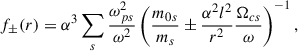
The solution of Eq. (50) establishes the pressure and density profiles that keep the plasma in radial equilibrium. Using P_s = β_sn_s^Γ_s, then the solution of that equation for density is

$$\begin{array}{c}\hfill n_s(r)={\left(\frac{{\mathrm{\Gamma }}_s-1}{{\mathrm{\Gamma }}_s{\beta }_s}\right)}^{\frac{1}{{\mathrm{\Gamma }}_s-1}}{[\frac{m_{0s}}{\alpha (r)}-m_s]}^{\frac{1}{{\mathrm{\Gamma }}_s-1}},\end{array}$$(51)

where m_0s is a constant with mass units. Different choices of m_0s determine the behavior of densities at infinities. For example, if every density species is required to vanish at infinity (n_s → 0 at r → ∞), then

$$\begin{array}{c}\hfill m_{0s}=m_s.\end{array}$$(52)

On the contrary, if each density species is required to be a constant n_0s at infinity (n_s → n_0s at r → ∞), then

$$\begin{array}{c}\hfill m_{0s}=m_s+\frac{{\mathrm{\Gamma }}_s{\beta }_s{n}_{0s}^{{\mathrm{\Gamma }}_s-1}}{{\mathrm{\Gamma }}_s-1}.\end{array}$$(53)

The value of β_s can be determined by the pressure, P_s(r₀), or density, n_s(r₀), at a reference radius; for example, r₀ = l.

On the other hand, in the mildly relativistic limit, the quasi-neutrality condition for an electron-ion plasma reduces simply to

$$\begin{array}{c}\hfill n_e=n_i,\end{array}$$(54)

which establishes a relation among the constants Γ_s, β_s, and m_0s of different species. For example, if the species have the same polytropic index, Γ, and their densities vanish at infinity, then from Eq. (51), we can find that the different constants, β_s, are related by

$$\begin{array}{c}\hfill \frac{{\beta }_i}{{\beta }_e}=\frac{m_i}{m_e}.\end{array}$$(55)

If the densities approach constant values at infinity, a quasi-neutral plasma is achieved when the condition given by Eq. (55) is satisfied, and when the constant densities also fulfill

$$\begin{array}{c}\hfill \frac{{\beta }_e{n}_{0e}^{\mathrm{\Gamma }-1}}{m_e}=\frac{{\beta }_i{n}_{0i}^{\mathrm{\Gamma }-1}}{m_i},\end{array}$$(56)

which establishes equal energies for electrons and ions at infinity. For a quasi-neutral electron-positron-ion plasma, we have n_e = n_p + n_i, so equivalent expressions can be straightforwardly derived.

3.4. Final equation for a mildly relativistic plasma

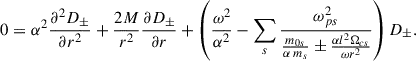
Using the density solution given by Eq. (51), Eq. (46) reduces to

$$\begin{array}{c}\hfill 0={\alpha }^2\frac{{\partial }^2{D}_{\pm }}{\partial r^2}+\frac{2M}{r^2}\frac{\partial D_{\pm }}{\partial r}+(\frac{{\omega }^2}{{\alpha }^2}-{\displaystyle \sum _s}\frac{{\omega }_{\mathit{ps}}^2}{\frac{m_{0s}}{\alpha m_s}\pm \frac{\alpha l^2{\mathrm{\Omega }}_{\mathit{cs}}}{\omega r^2}})D_{\pm }.\end{array}$$(57)

Finally, a major insight can be obtained by performing a change of variable to the tortoise coordinate modulated by the wave frequency,

$$\begin{array}{c}\hfill z=\omega (r+2Mln|\frac{r}{2M}-1|),\end{array}$$(58)

so that Eq. (57) can finally be put in the simpler form

$$\begin{array}{c}\hfill 0=\frac{{\partial }^2{D}_{\pm }}{\partial z^2}+(1-f_{\pm })D_{\pm },\end{array}$$(59)

where the dimensionless function, f_±, is

$$\begin{array}{c}\hfill f_{\pm }(r)={\alpha }^3{\displaystyle \sum _s}\frac{{\omega }_{\mathit{ps}}^2}{{\omega }^2}{\left(\frac{m_{0s}}{m_s}\pm \frac{{\alpha }^2{l}^2}{r^2}\frac{{\mathrm{\Omega }}_{\mathit{cs}}}{\omega }\right)}^{-1},\end{array}$$(60)

which needs to be evaluated in z.

Equation (59) determines the propagation of circularly polarized electromagnetic waves in plasmas in a Schwarzschild metric. The different propagation for the two polarizations of these circularly polarized waves is due to f₊ ≠ f₋. On the other hand, when the plasma is neglected, we recover the Schwarzschild vacuum redshift of light (see Appendix A). In general, our solution is satisfactory for exact dynamics in which the plasma is not moving radially (see Eq. (29)). The plasma can oscillate with velocities in the θ and ϕ directions, each of them altered by Faraday rotation according to Eqs. (44) and (48).

In the flat–space-time limit, α → 1 and r → l (as the background magnetic field is infinite and uniform), we recover the well-known result for Faraday rotation. However, in a Schwarzschild background, the Faraday rotation appears to be modified by the curvature through α and α²/r², which also includes the effect of gravitational redshift of light. This is an essential result of this work; any possible measurement of Faraday rotation of astrophysical objects that does not coincide with the flat–space-time result could indicate light propagation in a Schwarzschild curved space-time background. Thus, Faraday rotation can be used to obtain information on the mass of the astrophysical objects that produce such curvature. This may involve comparing two directions, one from the black hole and the other from a nearby source.

4. Flat–space-time solution

Let us first show that the previous system, described by Eq. (59), reduces to known results in the flat–space-time limit. When r → ∞, Eq. (59) becomes

$$\begin{array}{c}\hfill 0=\frac{{\partial }^2{D}_{\pm }}{\partial z^2}+(1-f_{0\pm })D_{\pm },\end{array}$$(61)

where

$$\begin{array}{c}\hfill f_{0\pm }={\displaystyle \sum _s}\frac{{\omega }_{ps0}^2}{{\omega }^2}{\left(\frac{m_{0s}}{m_s}\pm \frac{{\mathrm{\Omega }}_{\mathit{cs}}}{\omega }\right)}^{-1},\end{array}$$(62)

are just constants. Here ${\omega }_{ps0}=\sqrt{4\pi e^2{n}_{0s}/m_s}$ is the plasma frequency measured with constant density n_0s at infinity (i.e., in the flat–space-time limit case), with m_0s satisfying Eq. (53).

We can find an exact solution of Eq. (61). With the ansatz given by Eq. (40), the general solution reads $D_{\pm }=\alpha r{\mathcal{E}}_{\pm }=exp(i{\mathrm{\Psi }}_{\pm })$, so that the total phase is Ψ_± = ωt + S_0±, with

$$\begin{array}{c}\hfill S_{0\pm }=\sqrt{1-f_{0\pm }}z.\end{array}$$(63)

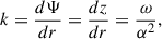
Calculating the frequency of the wave through the time derivative of the phase

$$\begin{array}{c}\hfill W=\frac{d{\mathrm{\Psi }}_{\pm }}{\mathit{dt}}=\omega ,\end{array}$$(64)

and the wavevector of the wave through the space derivative of the phase

$$\begin{array}{c}\hfill k_{\pm }=\frac{d{\mathrm{\Psi }}_{\pm }}{\mathit{dr}}=\frac{d{S}_{0\pm }}{\mathit{dr}}=\sqrt{1-f_{0\pm }}\frac{\mathit{dz}}{\mathit{dr}}=\omega \sqrt{1-f_{0\pm }},\end{array}$$(65)

we can find the dispersion relation for Faraday rotation in flat space-times,

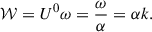
$$\begin{array}{c}\hfill {\omega }^2-{\displaystyle \sum _s}{\omega }_{ps0}^2{\left(\frac{m_{0s}}{m_s}\pm \frac{{\mathrm{\Omega }}_{\mathit{cs}}}{\omega }\right)}^{-1}=k_{\pm }^2,\end{array}$$(66)

corresponding to waves propagating in an adiabatic plasma. The flat–space-time dispersion relation (66) coincides with the previous findings in the case of an electron-positron plasma with densities vanishing at infinity (52) (see Appendix B).

5. Quasi-monochromatic wave solution

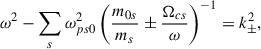
We can solve Eq. (59) in the Schwarzschild space-time under the quasi-monochromatic approximation for plasma wave propagation far from the black hole, r ≫ M. In this case,

$$\begin{array}{c}\hfill f_{\pm }\approx f_{0\pm }+\frac{2M}{r}{f}_{1\pm },\end{array}$$(67)

with f_0± given by Eq. (62), and f_1± a constant function given by

$$\begin{array}{cc}\hfill f_{1\pm }& ={\displaystyle \sum _s}\frac{{\omega }_{ps0}^2}{{\omega }^2}{\left(\frac{m_{0s}}{m_s}\pm \frac{{\mathrm{\Omega }}_{\mathit{cs}}}{\omega }\right)}^{-1}\hfill \\ \hfill & \times (\pm \frac{{\mathrm{\Omega }}_{\mathit{cs}}}{\omega (\frac{m_{0s}}{m_s}\pm \frac{{\mathrm{\Omega }}_{\mathit{cs}}}{\omega })}+\frac{m_s}{2\mathrm{\Gamma }{\beta }_s{n}_{0s}^{\mathrm{\Gamma }-1}}-\frac{3}{2}+\frac{1}{2(\mathrm{\Gamma }-1)}),\hfill \end{array}$$(68)

for a plasma with constant density at infinity, i.e., in the flat–space-time limit case.

Let us look for a solution of the form

$$\begin{array}{c}\hfill D_{\pm }=(1+\frac{{ϵ}_{\pm }}{2})exp\left(i{S}_{\pm }\right),\end{array}$$(69)

with the generalized phase

$$\begin{array}{c}\hfill S_{\pm }=\sqrt{1-f_{0\pm }}(z-{\displaystyle \int {ϵ}_{\pm }}dz)\end{array}$$(70)

and real ϵ_± ≪ 1. These expressions and approximations are used to construct an approximate analytical solution to the radially dependent phase, S_±(r), using the WKB (eikonal) approximation described in Eq. (69).

At first order, Eq. (59) reduces to

$$\begin{array}{c}\hfill \frac{d^2{ϵ}_{\pm }}{d{z}^2}+4(1-f_{0\pm }){ϵ}_{\pm }=\frac{4M{f}_{1\pm }}{r},\end{array}$$(71)

where 1/r must be evaluated in terms of z given by Eq. (58). The general solution to the above equation is

$$\begin{array}{cc}& {ϵ}_{\pm }(z)=\frac{2M\omega f_{1\pm }}{\sqrt{1-f_{0\pm }}}\hfill \\ \hfill & \times [sin\left(2\sqrt{1-f_{0\pm }}z\right){\chi }_{\pm }(z)-cos\left(2\sqrt{1-f_{0\pm }}z\right){\mathrm{\Lambda }}_{\pm }(z)],\hfill \end{array}$$(72)

where

$$\begin{array}{cc}\hfill {\chi }_{\pm }(z)& ={\displaystyle {\int }_z}\frac{cos\left[2\omega \sqrt{1-f_{0\pm }}(y+2Mln|\frac{y}{2M}-1|)\right]}{y-2M}dy,\hfill \\ \hfill {\mathrm{\Lambda }}_{\pm }(z)& ={\displaystyle {\int }_z}\frac{sin\left[2\omega \sqrt{1-f_{0\pm }}(y+2Mln|\frac{y}{2M}-1|)\right]}{y-2M}dy.\hfill \end{array}$$(73)

Furthermore, a simple approximated solution of Eq. (71) can be found far from the black hole when z ≈ ωr. In this case, we have

$$\begin{array}{c}\hfill {ϵ}_{\pm }={\displaystyle \sum _{n=0}^{\infty }}\frac{{\delta }_n^{\pm }}{z^{2n+1}},\end{array}$$(74)

where

$$\begin{array}{cc}\hfill {\delta }_0^{\pm }& =\frac{M\omega f_{1\pm }}{1-f_{0\pm }},\hfill \\ \hfill {\delta }_{n+1}^{\pm }& =-\frac{(2n+1)(n+1)}{2(1-f_{0\pm })}{\delta }_n^{\pm }.\hfill \end{array}$$(75)

With the above solution, we can obtain a proper analytical expression for the Faraday rotation of electromagnetic waves far from the black hole, accounting for its gravitational effect.

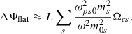
6. Faraday rotation for quasi-monochromatic electromagnetic waves far from the black hole

Because the two polarizations have different dispersions, an initially linearly polarized wave experiences a rotation, ΔΨ, of its plane of polarization that increases with the distance traveled by the wave. The angle of rotation is proportional to the arctan of the ratio between the two components of the electric field. For any point in space-time, the polarization angle of the wave is proportional to the difference of phases of the two polarizations, δΨ ∝ ΔS = S₊ − S₋. Thus, for any path traveled by the electromagnetic wave, the total polarization angle of rotation is given by ΔΨ  ≈ ∫∂_rΔSdr = ∫(∂_rS₊ − ∂_rS₋)dr, where the integration is along the path. In our case, the total rotation angle can be calculated from Eq. (70) to give

$$\begin{array}{c}\hfill \mathrm{\Delta }\mathrm{\Psi }\approx {\displaystyle {\int }_{2M}^L}\frac{\omega }{{\alpha }^2}[\sqrt{1-f_{0+}}(1-{ϵ}_{+})-\sqrt{1-f_{0-}}(1-{ϵ}_{-})]dr,\end{array}$$(76)

where L ⋙ 2M is the total radial length (far from the black hole) traveled by the wave. Here ω appears by the variable change. Two space-time curvature effects modify (in general) the rotation angle. The first is the α⁻² factor, associated with the gravitational redshift of the light wave’s phase. The observed frequency (measured by an observer at rest) can be obtained straightforwardly (see the appendix). The second effect is associated with the coupling between space-time curvature and the wave’s extended nature. This modifies the propagation properties of the wave through ϵ_± in the amplitude and phase, as is shown in Eq. (69).

When S₊ = S₋, there is no Faraday rotation with ΔΨ = 0. On the contrary, for propagation in flat–space-time (with ϵ_± = 0), we obtain

$$\begin{array}{c}\hfill \mathrm{\Delta }{\mathrm{\Psi }}_{\mathrm{flat}}\approx L\omega (\sqrt{1-f_{0+}}-\sqrt{1-f_{0-}}).\end{array}$$(77)

For high-frequency waves and weakly magnetized plasmas (1 ≫ f_0±), the well-known result is recovered (Kulsrud 2005):

$$\begin{array}{c}\hfill \mathrm{\Delta }{\mathrm{\Psi }}_{\mathrm{flat}}\approx L{\displaystyle \sum _s}\frac{{\omega }_{ps0}^2{m}_s^2}{{\omega }^2{m}_{0s}^2}{\mathrm{\Omega }}_{\mathit{cs}}.\end{array}$$(78)

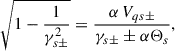
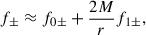
In the case of electromagnetic waves propagating in plasmas in a Schwarzschild background, we can use solutions (74) to evaluate the Faraday rotation (76). Very far from the black hole (L ⋙ 2M), we get

$$\begin{array}{c}\hfill \mathrm{\Delta }\mathrm{\Psi }\approx \mathrm{\Delta }{\mathrm{\Psi }}_{\mathrm{flat}}-\omega Lln\left(\frac{L}{2M}\right)(\sqrt{1-f_{0+}}{\delta }_0^{+}-\sqrt{1-f_{0-}}{\delta }_0^{-}).\end{array}$$(79)

The rotation angle includes curvature effects through the appearance of the black hole mass. The angle contains effects arising from the coupling between the polarization and the gravitational field via δ₀^±. These effects differ from the standard redshift, as they appear when electromagnetic wave propagation is considered beyond the geometrical optics approximation, i.e., for quasi-monochromatic waves.

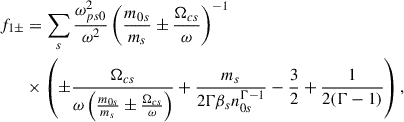
For propagation far from the black hole, we can use Eq. (75) to explicitly evaluate the angle in Eq. (79). Then, for high-frequency waves in the weakly magnetized limit and high-density regime, n₀^Γ − 1 ≫ m_s, we have

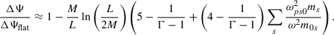$$\begin{array}{c}\hfill \frac{\mathrm{\Delta }\mathrm{\Psi }}{\mathrm{\Delta }{\mathrm{\Psi }}_{\mathrm{flat}}}\approx 1-\frac{M}{L}ln\left(\frac{L}{2M}\right)(5-\frac{1}{\mathrm{\Gamma }-1}+(4-\frac{1}{\mathrm{\Gamma }-1}){\displaystyle \sum _s}\frac{{\omega }_{ps0}^2{m}_s}{{\omega }^2{m}_{0s}}).\end{array}$$(80)

In the gravitational correction to Faraday rotation, in a weakly magnetized plasma far from the black hole, the curvature couples with the plasma frequency, while the magnetic field only appears through ΔΨ_flat. This term, proportional to the ratio between the black hole mass, M, and the distance to the black hole, L, is a combination of the two effects that a wave can experience during its propagation on a Schwarzschild space-time: the redshift owed to its propagation along the gravitational pull, and the coupling between its polarization and curvature due to the extended nature of the wave in space-time. The total new contribution due to the polarization of the electromagnetic wave by the gravitational field decreases as the wave propagates farther from the black hole.

7. Discussion

Our final results, (Eqs. (79) and (80)), show how gravity, in particular a Schwarzschild space-time, modifies the magnetically induced Faraday rotation. In general, the corrections induced by the space-time curvature are coupled to polarization. A measure of the Faraday rotation could show this effect in the difference between the propagation of right-handed and left-handed electromagnetic polarized waves. As the effect of Schwarzschild curvature decreases with the distance, the impact of this coupling on Faraday rotation is proportional to 2M/r, as in Eq. (80). This solution is dependent on the condition given by Eq. (29) for plasmas with no radial velocity, u_s = 0. If this constraint is relaxed, while all the other conditions remain, we can find from the continuity equation, Eq. (24), that, in general, for every plasma species, r²αγ_sn_su_s = constant. Considering our approximations, for wave propagation far from the black hole, the above condition becomes r²n_0su_s = constant, where each density species is a constant n_0s at infinity. In that case, the only possible behavior for the radial velocity is u_s ∝ r⁻², decaying (far from the black hole) faster than the gravitational effect of this space-time curvature. Therefore, our assumption in Eq. (29) (u_s = 0), although it was initially considered for simplicity, is well justified for the plasma dynamics far from the black hole.

It is important to remark that the second and third terms in the Faraday rotation effect given by Eqs. (79) and (80) are pure general relativistic effects that can only occur in the presence of a plasma. The kind of magnetically induced Faraday rotation that we are proposing in this work, due to the interplay of electromagnetism, charged particles, and gravity, is different from the GFR effects, i.e., when only gravitational fields are considered. The latter cannot occur in a static Schwarzschild background (as it needs a rotational space-time). In contrast, the former effect can occur in static space-times because the magnetized plasma breaks radial symmetry. This is one of the major novelties introduced in the work. As the Faraday rotation (Eq. (80)) is present for radial propagation far from the black hole, it is independent of other relativistic effects, such as light bending.

In principle, the gravitational correction given by Eq. (80) for high-frequency electromagnetic waves (for the case when ω ∼ k_± ≫ ω_ps0) is on the order of |ΔΨ/ΔΨ_flat−1| ∼ (M/L)ln(L/2M). This can be estimated by noticing that

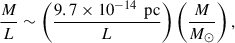$$\begin{array}{c}\hfill \frac{M}{L}\sim \left(\frac{9.7\times {10}^{-14}\text{pc}}{L}\right)\left(\frac{M}{M_{\odot }}\right),\end{array}$$(81)

for black hole masses measured in solar masses, M_⊙, and distance, L, measured in parsecs. For instance, for the supermassive black hole M87 (The Event Horizon Telescope Collaboration 2019), at 16.8 Mpc and with a mass of 6.5 × 10⁹ M_⊙, we find |ΔΨ/ΔΨ_flat−1| ∼ 8.8 × 10⁻¹⁰. A similar order of magnitude can be estimated for the black hole in Sgr A* at the center of our galaxy. These corrections are quite small, since they were required to obtain the approximated analytical solution for quasi-monochromatic waves in Sect. 5. Physically, this means that the effect of the Schwarzschild space-time on the Faraday rotation of quasi-monochromatic plane waves is not very sensitive to the supermassive black holes we can observe today. However, this does not imply that the effect does not exist or lacks importance. The proper behavior of Faraday rotation for electromagnetic waves in a plasma closer to the event horizon or for more general electromagnetic wave propagation cannot be studied by considering just quasi-monochromatic plane wave solutions shown in Sect. 5. They must be studied numerically by solving Eq. (59). It is expected that when the complete system is studied (by abandoning the quasi-monochromatic approximation), a larger effect due to the gravitational field should appear in the plasma Faraday rotation. The same conclusion would apply if conditions (29)–(32) are relaxed. The complete study of the system and of Eq. (59), together with its general propagation, can only be performed numerically. This will be left for future studies.

Despite that, and bringing our attention back to the solution given in Eq. (80), we can see that far from the black hole any measurement that does not coincide with the flat Faraday rotation value (Eq. (78)) can provide information about the properties of the curved space-time. For example, several measurements at different frequencies can be performed to determine the mass, M, of a black hole interacting with a propagating electromagnetic wave. However, it is important to notice that an excellent knowledge of ΔΨ_flat is needed to evaluate, in an appropriate manner, the result shown in Eq. (80). In future work, we plan to estimate the coupling between the geometry and the magnetic field in the highly magnetized case, which could be interesting in some situations, such as magnetars. Similarly, the above analysis can also be performed for other metrics, finding corrections to Faraday rotation for light from Kerr black holes or more general cosmologies, such as Bianchi-I space-times.

Acknowledgments

The authors thank Pedro Godoy for his valuable comments on our work. F.A.A. thanks Fondecyt-Chile grant No. 1230094. P.S.M. thanks Fondecyt-Chile grant No. 1240281 and the support of the Research Vice-rectory of the University of Chile (VID) through grant ENL08/23. V. M. thanks Fondecyt-Chile grant No. 1161711. J.A.V. thanks the support of Fondecyt project No. 1240697 and CEDENNA under Conicyt Basal Program Grant FB0807.

References

Appendix A: Vacuum redshift

When the plasma is neglected in Eq. (59), then n_s = 0 and f_± = 0. The solution of (59) is exact and becomes simply D_± = exp(iz). The general solution for the electromagnetic wave is E_± = (1/αr)exp(iΨ), the total phase

$$\begin{array}{c}\hfill \mathrm{\Psi }=\omega t+z,\end{array}$$(A.1)

which results is independence from polarization, as expected. The frequency of the wave is calculated through the time derivative of the phase

$$\begin{array}{c}\hfill \frac{d\mathrm{\Psi }}{\mathit{dt}}=\omega ,\end{array}$$(A.2)

while the wavevector of the wave is

$$\begin{array}{c}\hfill k=\frac{d\mathrm{\Psi }}{\mathit{dr}}=\frac{\mathit{dz}}{\mathit{dr}}=\frac{\omega }{{\alpha }^2},\end{array}$$(A.3)

finding that ω = α²k. By defining the four-wavevector K_μ = ∂_μΨ, an observer at rest with timelike vector four-velocity U^μ, such that Uⁱ = 0 and U^μU_μ = −1, measures a frequency $\mathcal{W}=U^{\mu }{K}_{\mu }$ resulting to be

$$\begin{array}{c}\hfill \mathcal{W}=U^0\omega =\frac{\omega }{\alpha }=\alpha k.\end{array}$$(A.4)

This defines the usual Schwarzschild redshift experienced by light in vacuum measured by an observer at rest.

Appendix B: Flat–space-time dispersion relation

The flat–space-time dispersion relation (66) agrees with several previous results, under different conditions, when different densities vanish at infinity.

In Sakai & Kawata (1980), the dispersion relation (k/ω)² = 1 − 2ω_p²/(ω² − Ω_c²) is found for transverse electron-positron plasma waves propagating parallel to a constant magnetic field. The same dispersion relation is found in Eq. (11) in Asenjo et al. (2009) when low temperature and sub-relativistic velocities are considered. This dispersion relation concurs with Eq. (66).

Similarly, the dispersion relation found in Buzzi et al. (1995) for an electron-positron plasma (where r_H is the scale gradient of the lapse function on the local approximation)

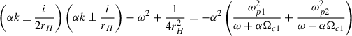$$\begin{array}{c}\hfill (\alpha k\pm \frac{i}{2r_H})(\alpha k\pm \frac{i}{r_H})-{\omega }^2+\frac{1}{4r_H^2}=-{\alpha }^2(\frac{{\omega }_{p1}^2}{\omega +\alpha {\mathrm{\Omega }}_{c1}}+\frac{{\omega }_{p2}^2}{\omega -\alpha {\mathrm{\Omega }}_{c1}})\end{array}$$(B.1)

coincides with dispersion relation given by Eq. (66) in the limit of the wavelength of the plasma wave being much smaller than r_H, and no background plasma velocity.

References

- Asada, K., Inoue, M., Uchida, Y., et al. 2002, PASJ, 54, L39 [NASA ADS] [Google Scholar]
- Asada, K., Inoue, M., Kameno, S., et al. 2008, ApJ, 675, 79 [Google Scholar]
- Asenjo, F. A., Muñoz, V., Valdivia, J. A., & Hada, T. 2009, Phys. Plasmas, 16, 122108 [Google Scholar]
- Asenjo, F. A., Mahajan, S. A., & Qadir, A. 2013, Phys. Plasmas, 20, 022901 [NASA ADS] [CrossRef] [Google Scholar]
- Attridge, J. M., Wardle, J. F. C., & Homan, D. C. 2005, ApJ, 633, L85 [Google Scholar]
- Broderick, A., & Blandford, R. 2003, MNRAS, 342, 1280 [Google Scholar]
- Buzzi, V., Hines, K. C., & Treumann, R. A. 1995, Phys. Rev. D, 51, 6663 [Google Scholar]
- Campanelli, L., Dolgov, A. D., Giannotti, M., et al. 2004, ApJ, 616, 1 [Google Scholar]
- Chandrasekhar, S. 1983, The Mathematical Theory of Black Holes (Oxford: Clarendon Press) [Google Scholar]
- Chen, F. F. 1984, Introduction to Plasma Physics and Controlled Fusion (New York: Plenum Press) [Google Scholar]
- Connors, P. A., & Stark, R. F. 1977, Nature, 269, 128 [Google Scholar]
- Connors, P. A., Piran, T., & Stark, R. F. 1980, ApJ, 235, 224 [Google Scholar]
- Dehnen, H. 1973, Int. Jour. Theo. Phys., 7, 467 [Google Scholar]
- Dreher, J. W., Carilli, C. L., & Perley, R. A. 1987, ApJ, 316, 611 [NASA ADS] [CrossRef] [Google Scholar]
- Frolov, V. P., & Koek, A. 2024, Phys. Rev. D, 110, 064052 [Google Scholar]
- Gaensler, B. M., Haverkorn, M., Stateveley-Smith, L., et al. 2005, Science, 307, 1610 [NASA ADS] [CrossRef] [Google Scholar]
- Han, J. L., Manchester, R. N., Lyne, A. G., Qiao, G. J., & van Straten, W. 2006, ApJ, 642, 868 [Google Scholar]
- Ishihara, H., Takahashi, T., Tomimatsu, A., et al. 1988, Phys. Rev. D, 38, 472 [Google Scholar]
- Kosowsky, A., & Loeb, A. 1996, ApJ, 469, 1 [Google Scholar]
- Krall, N. A., & Trivelpiece, A. W. 1973, Principles of Plasma Physics (New York: McGraw-Hill Inc.) [Google Scholar]
- Kulsrud, R. M. 2005, Plasma Physics for Astrophysics (Princeton: Princeton University Press) [Google Scholar]
- Murgia, M., Govoni, F., Feretti, L., et al. 2004, A&A, 424, 429 [NASA ADS] [CrossRef] [EDP Sciences] [Google Scholar]
- Nouri-Zonoz, M. 1999, Phys. Rev. D, 60, 024013 [Google Scholar]
- Park, K., & Blackman, E. G. 2010, MNRAS, 403, 1993 [Google Scholar]
- Parker, L. 1969, Am. J. Phys., 37, 313 [Google Scholar]
- Plebanski, J. 1960, Phys. Rev., 118, 1396 [Google Scholar]
- Pshirkov, M. S., Tinyakov, P. G., Kronberg, P. P., et al. 2011, ApJ, 738, 192 [NASA ADS] [CrossRef] [Google Scholar]
- Sakai, J., & Kawata, T. 1980, J. Phys. Soc. Japan, 49, 747 [Google Scholar]
- Sereno, M. 2004, Phys. Rev. D, 69, 087501 [Google Scholar]
- Simard-Normandin, M., Kronberg, P. P., & Button, S. 1981, ApJ, 45, 97 [Google Scholar]
- Tamburini, F., Thidé, B., Molina-Terriza, G., et al. 2011, Nat. Phys., 7, 195 [Google Scholar]
- The Event Horizon Telescope Collaboration 2019, ApJ, 875, L1 [Google Scholar]
- Thorne, K. S., Price, R. H., & Macdonald, D. A. 1986, Black Holes: The Membrane Paradigm (New Haven and London: Yale University Press) [Google Scholar]
- Xu, Y., Kronberg, P. P., Habib, S., et al. 2005, ApJ, 637, 19 [Google Scholar]
- Zavala, R. T., & Taylor, G. B. 2005, ApJ, 626, L73 [Google Scholar]