| Issue |
A&A
Volume 706, February 2026
|
|
|---|---|---|
| Article Number | A77 | |
| Number of page(s) | 25 | |
| Section | Numerical methods and codes | |
| DOI | https://doi.org/10.1051/0004-6361/202555356 | |
| Published online | 03 February 2026 | |
Accelerating the CLEAN algorithm of radio interferometry with convex optimization
1
Max-Planck-Institut für Radioastronomie,
Auf dem Hügel 69,
53121
Bonn,
Germany
2
National Radio Astronomy Observatory,
PO Box O,
Socorro,
NM
87801,
USA
★ Corresponding author: This email address is being protected from spambots. You need JavaScript enabled to view it.
Received:
30
April
2025
Accepted:
21
November
2025
Abstract
Context. In radio interferometry, images are recovered from incompletely sampled Fourier datasets. The de facto standard algorithm, the Cotton–Schwab CLEAN, iteratively switches between computing a deconvolution (minor loop) and subtracting the model from the visibilities (major loop).
Aims. The next generation of radio interferometers is expected to handle much higher data rates, image sizes, and sensitivity, making acceleration of current data processing algorithms necessary. We aim to achieve this by evaluating the potential of various well-known acceleration techniques in convex optimization for the major loop. For the present manuscript, we limit our study of these techniques to the CLEAN framework.
Methods. To this end, we identify CLEAN with a Newton scheme and work backwards through this chain of arguments to express Nesterov acceleration and conjugate gradient orthogonalization in the major and minor loop framework.
Results. The resulting algorithms are simple extensions of the traditional framework. However, they converge multiple times faster than traditional techniques and reduce the residual significantly deeper. These improvements achieved by accelerating the major loop are competitive with other well-known improvements by replacing the minor loop with more advanced algorithms, but at lower numerical cost. The best performance is achieved by combining these two developments.
Conclusions. CLEAN remains among the fastest and most robust algorithms for imaging in radio interferometry and can be easily extended to achieve an order of magnitude faster convergence speed and dynamic range. The procedure outlined in this manuscript is relatively straightforward and could be easily extended.
Key words: methods: numerical / techniques: image processing / techniques: interferometric
© The Authors 2026
 Open Access article, published by EDP Sciences, under the terms of the Creative Commons Attribution License (https://creativecommons.org/licenses/by/4.0), which permits unrestricted use, distribution, and reproduction in any medium, provided the original work is properly cited.
This article is published in open access under the Subscribe to Open model.
Open Access funding provided by Max Planck Society.
1 Introduction
The observables in a radio interferometer are the correlated (and time-shifted) signals recorded at individual antennas. These are approximately related to on-sky emission through a Fourier transform as described by the van-Cittert–Zernike theorem (Thompson et al. 2017). For data processing in radio interferometric imaging, an image must be reconstructed from sparsely sampled (on a non-equidistant grid), noisy Fourier coefficients (called visibilities). Equivalently, this problem is reformulated as a deconvolution problem in which the residual map – defined as the inverse Fourier transform of the visibilities – needs to be de-convolved with the beam, which is the inverse Fourier transform of the sampling pattern (also called the point spread function).
Historically, the imaging problem has been solved by the CLEAN algorithm (Högbom 1974), a matching pursuit algorithm in which the image is inversely modeled by the subtraction of individual model components from the residual. Iteratively, the algorithm searches for the maximum in the current residual, shifts the beam to that location, and subtracts a fraction of the beam. In this way, the emission is modeled iteratively by delta components. The CLEAN algorithm has been further developed and modernized into multi-scalar and multifrequency variants (Bhatnagar & Cornwell 2004; Cornwell 2008; Rau & Cornwell 2011; Offringa et al. 2014; Offringa & Smirnov 2017; Müller & Lobanov 2023b; Müller & Bhatnagar 2025). In its most common implementation – for example, as available from the CASA package (CASA Team 2022) – the CLEAN algorithm operates in the image domain. We refer to this iterative procedure of deconvolution as the minor loop. Data consistency is ensured by an external loop (referred to as the major loop). The residual is updated by Fourier transforming and degridding the current image model, comparing it with the observed visibilities, and subsequently gridding and inverse Fourier transforming the resulting difference of the visibilities. As first proposed by Schwab (1984), one typically alternates between these two steps (computing the deconvolution and updating the residual). Since these two steps are inherently linked to each other, we refer to the combination of major loop and minor loop as the CLEAN algorithm for the remainder of this manuscript.
A wide range of alternative imaging approaches has been suggested in the past, including the Maximum-Entropy Method (Cornwell & Evans 1985), regularized maximum-likelihood (e.g., Akiyama et al. 2017; Chael et al. 2018; Müller et al. 2023; Mus et al. 2024), compressive sensing (e.g., Starck et al. 1994; Wiaux et al. 2009; Garsden et al. 2015; Onose et al. 2017; Müller & Lobanov 2022, 2023a), Bayesian approaches (e.g., Junklewitz et al. 2016; Broderick et al. 2020; Arras et al. 2021), and recently AI-based ideas (e.g., Connor et al. 2022; Sun et al. 2022; Aghabiglou et al. 2024). Most of these approaches formulate the problem as a forward-modeling problem. Forward modeling describes the process by which the sought-after signal is mapped and solved in a statistically consistent manner. Here we use the common term forward modeling to highlight the difference between the strategy of including the instrumental response directly in the forward operator, as opposed to correcting inversely for instrumental, calibration, and gridding effects and projecting them onto the image domain (the strategy applied by most CLEAN implementations through the major and minor loop). However, the terminology should not cause confusion: the CLEAN algorithm is a forward-modeling algorithm that ensures data compatibility through the major loop.
These techniques address several key limitations of the CLEAN approach. Unlike CLEAN, which implicitly encodes regularization within the algorithm and by user-based choices, forward-modeling methods optimize well-defined objective functions. They also provide a natural framework for joint calibration and deconvolution, adapt well to cases where the forward operator becomes nonlinear, and incorporate uncertainty quantification. Moreover, they resolve the inherent dichotomy in CLEAN between the model (a set of CLEAN components) and the final image (components convolved with the clean beam). The forward formulation further allows the inclusion of more sophisticated prior information than assuming a sparse set of CLEAN components – for example, through prior distributions, explicit regularizers, or learned or inferred features. As a result, several science cases have demonstrated that forward-modeling approaches can outperform CLEAN-based methods in terms of dynamic range and resolution (e.g., Arras et al. 2021; Dabbech et al. 2024), although opposite findings have also been reported (Offringa & Smirnov 2017; Bester et al. 2026). A notable area where CLEAN is increasingly supplanted by forward-modeling techniques is global millimeter-wavelength Very Long Baseline Interferometry (VLBI), where the limited number of antennas and modest signal-to-noise ratios pose particular challenges. Nonetheless, CLEAN remains applicable and widely used in such settings as well (e.g., Event Horizon Telescope Collaboration 2019, 2021, 2022; Lu et al. 2023; Event Horizon Telescope Collaboration 2024).
Despite these developments, CLEAN remains the standard method in radio interferometry. This is mainly because of its maturity, robustness, adaptivity, and speed. Its speed is achieved through its rather simple deconvolution procedure, which mostly includes steps of only linear numerical complexity that do not scaling with the number of visibilities, along with splitting the data analysis problem into the major and minor loops. Notably, the latter idea has been recently adapted to accelerate Bayesian (Roth et al. 2024) and AI-based imaging (Aghabiglou et al. 2024) as well, achieving up to an order-of-magnitude speedup.
Alternative approaches, despite their suggestive performance and precision, have not yet enjoyed widespread application on an observatory level. This is partly due to the significant development required to mature these approaches into application-ready, automated pipelines that robustly adapt to all observing modes, science cases, and source structures accessible to an instrument. Moreover, CLEAN implementations have also seen substantial development in recent years (Hsieh & Bhatnagar 2021; Hsieh et al. 2022b; Müller & Lobanov 2023b; Müller & Bhatnagar 2025; Jarret et al. 2025), mimicking some performance gains claimed by alternative approaches.
A new generation of radio interferometers is either under development or actively planned, including the Square Kilometre Array (SKA Dewdney et al. 2009), the next-generation Very Large Array (ngVLA Murphy et al. 2018; Selina et al. 2018), and the DSA-2000 (Hallinan et al. 2019). Additionally, the Atacama Large Millimeter/submillimeter Array (ALMA) is slated for significant enhancement through its wideband sensitivity upgrade (WSU Carpenter et al. 2022). These next-generation instruments will operate at substantially higher data rates and with markedly improved sensitivity. These advancements introduce considerable challenges for data processing. In particular, all imaging and calibration techniques must scale effectively to accommodate the data volumes produced by these arrays. Furthermore, standard simplifying assumptions, such as representing the sky brightness distribution using point source models, may no longer be valid. This necessitates the development and deployment of more computationally intensive and sophisticated algorithms.
Gridding likely drives numerical cost, as demonstrated by Bhatnagar et al. (2021, 2022). This indeed questions the use of many forward-modeling approaches, despite their superior dynamic range demonstrated in a few test cases, which under-pins recent efforts to recast them within an efficient minor and major loop skeleton. Scalability is the paramount priority and requirement for the construction of next-generation data processing pipelines (Bhatnagar et al. 2022; Kepley et al. 2023; Hunter et al. 2023; Bhatnagar et al. 2025). Improved resolution and dynamic range would benefit many science cases, but the majority of observational data, especially the large mosaics and surveys that dominate numerical cost in observatory-driven automated pipelines, remain well served by CLEAN variants (see, e.g., the discussions in Kepley et al. 2023; Bester et al. 2026). As a consequence, multi-scale variants of CLEAN, shown to perform well, quickly, and robustly, remain among the preferred choices for constructing pipelines for these arrays and are under active development and deployment by observatories (e.g., Hsieh & Bhatnagar 2021; Hsieh et al. 2022a; CASA Team 2022; Hunter et al. 2023; Bhatnagar et al. 2025).
Despite its remarkable longevity, CLEAN operates within a relatively simple optimization framework, without making use of accelerating techniques that have become popular over the last two decades. Regularized maximum likelihood and compressive sensing, which directly formulate the problem as an optimization problem, have developed and utilized more advanced settings. In this manuscript, we aim to combine these two approaches, i.e., we apply concepts of accelerating numerical optimization to the classical CLEAN framework. As a result, we construct algorithms based on the robust and proven framework of CLEAN that converge faster in terms of the number of major loop iterations, significantly reducing computational time.
This is first done by formulating CLEAN in the common language of optimization and then, in the opposite logical direction, deriving CLEAN alternatives within accelerated optimization algorithms. The manuscript is structured along this logic. We first discuss in Sect. 2 how CLEAN can be understood as an optimization technique, then in Sect. 3 how to formulate these optimization techniques within the CLEAN framework. We show results on synthetic and real data applications in Sects. 4 and 5, and present our conclusions in Sect. 6.
2 CLEAN as an optimization technique
2.1 Radio interferometry
The correlated signal between two antennas is approximately the Fourier transform of the on-sky emission I(l, m):
![Mathematical equation: $\[\mathcal{V}(u, v)=\int\int I(l, m) e^{-2 \pi i(l u+m v)} d l d m.\]$](/articles/aa/full_html/2026/02/aa55356-25/aa55356-25-eq1.png) (1)
(1)
Here, 𝒱 denotes the visibilities (the measurements), u, v are harmonic coordinates, and l, m are direction cosines on-sky. In practice, only a sparse subset of the visibilities is measured, the visibilities are corrupted by thermal noise as well as station-based and direction-dependent calibration effects. All of these operations are summarized in the following radio interferometry measurement equation (Hamaker et al. 1996; Smirnov 2011):
![Mathematical equation: $\[\begin{aligned}V_{i j}(t)= & G_i(t)\left(\int_{\Omega} E_i(\hat{s}, t) I(\hat{s}, t) E_j^{\dagger}(\hat{s}, t) e^{-2 \pi i u_{i j} \cdot \hat{s}} \mathrm{~d} \Omega\right) G_j^{\dagger}(t) \\& +\epsilon_{i j}(t).\end{aligned}\]$](/articles/aa/full_html/2026/02/aa55356-25/aa55356-25-eq2.png) (2)
(2)
Here Gi and Gj describe direction-independent gains, Ei and Ej denote direction-dependent gains, and ϵ represents additive thermal noise.
An important numerical complexity stems from the fact that the visibilities are not taken on an equidistant grid. Computing the residual and the dirty beam therefore includes more operations than the simple application of the fast Fourier transform (FFT). We first have to convolve the measured visibilities in the Fourier domain with a gridding kernel before applying an inverse FFT, and then correct for this convolution in the image domain (normalization). This procedure is typically referred to as gridding.
For the remainder of the manuscript, we denote the discretized version of the measurement operator by Φ and study the problem:
![Mathematical equation: $\[V=\Phi I+\epsilon.\]$](/articles/aa/full_html/2026/02/aa55356-25/aa55356-25-eq3.png) (3)
(3)
We refer to Bester et al. (2026); Bhatnagar et al. (2025) for a detailed derivation of the matrix form of Φ. The measurement operator Φ is a rank-deficient matrix. We denote the transposed matrix of Φ by ΦT throughout this manuscript.
The data fidelity between a current guess solution Ik and the observed visibilities is described by the χ2-metric:
![Mathematical equation: $\[\chi^2\left(V, I_k\right)=\sum_i \frac{\|\left(V\left(u_i, v_i\right)-\left(\Phi I_k\right)\left(u_i, v_i\right) \|^2\right.}{\sigma_i^2},\]$](/articles/aa/full_html/2026/02/aa55356-25/aa55356-25-eq4.png) (4)
(4)
where the index i runs over all observed visibility points and σ is the associated thermal noise level. In fact, this data fidelity would correspond to natural weighting. It is common practice to re-weight the visibility data points to enhance specific spatial features. For example, the uniform weighting of all data points leads to higher resolution at the cost of sensitivity. A detailed description of common weighting schemes and their effect is provided by Briggs (1995). We do not dive deeper into this topic here and rather assume that all weightings and tapers applied to the data are fully described by a fixed array of weights σ.
In the following, we denote the domain of the operator Φ by X (i.e., the image plane), and its co-domain by Y, i.e.,
![Mathematical equation: $\[\Phi: \mathbf{X} \rightarrow \mathbf{Y},\]$](/articles/aa/full_html/2026/02/aa55356-25/aa55356-25-eq5.png) (5)
(5)
and equip the co-domain with the topology described by the Gram matrix ![Mathematical equation: $\[G_{\mathbf{Y}}=\operatorname{diag} 1 / \sigma_{i}^{2}\]$](/articles/aa/full_html/2026/02/aa55356-25/aa55356-25-eq6.png) . With this topology, we define the χ2 objective functional as
. With this topology, we define the χ2 objective functional as
![Mathematical equation: $\[J: \theta \mapsto \frac{1}{2}\|V-\Phi \theta\|_{\mathbf{Y}}^2.\]$](/articles/aa/full_html/2026/02/aa55356-25/aa55356-25-eq7.png) (6)
(6)
Since for an arbitrary vector r we obtain ![Mathematical equation: $\[\|r\|_{\mathbf{Y}}^{2}=\langle r, r\rangle_{\mathbf{Y}}=r^{+} G_{\mathbf{Y}} r\]$](/articles/aa/full_html/2026/02/aa55356-25/aa55356-25-eq8.png) , it is easy to show that J(θ) = 1/2 · χ2(V, θ) holds. We denote the adjoint Φ with respect to that topology by Φ+ = ΦTGY.
, it is easy to show that J(θ) = 1/2 · χ2(V, θ) holds. We denote the adjoint Φ with respect to that topology by Φ+ = ΦTGY.
2.2 Cotton–Schwab algorithm
The so-called Cotton–Schwab algorithm (Schwab 1984) splits the imaging problem into a major loop and minor loop. It is the de facto standard algorithm used in radio interferometry. We refer to this setup simply as CLEAN in the remainder of this manuscript.
A major loop iteration updates the current residual with the current guess solution Ik at iteration k, i.e., by degridding the model, comparing it to the observed visibilities, gridding the difference, and evaluating the inverse FFT. In the notation of the operators Φ and Φ+introduced in the previous subsection, this may be formulated by the operation,
![Mathematical equation: $\[I_k \mapsto \Phi^{+}\left(V-\Phi I_k\right).\]$](/articles/aa/full_html/2026/02/aa55356-25/aa55356-25-eq9.png) (7)
(7)
In the minor loop, we aim to model the image structure. We reformulate Eq. (3) as a deconvolution problem:
![Mathematical equation: $\[I^{r e s}=B * I_k+N,\]$](/articles/aa/full_html/2026/02/aa55356-25/aa55356-25-eq10.png) (8)
(8)
where Ires := Φ+V, B := Φ+ Φ, and N := Φ+ ϵ. Here, Ires is called the residual, and B the beam (the inverse Fourier transform of the sampling pattern). The beam (also called the point spread function) can also be interpreted as the response to a point source. We use these notations for the remainder of this manuscript.
A minor loop iteration consists of finding the peak in the current residual, shifting the beam to that position, subtracting a fraction of the shifted beam from the residual, and storing the position and strengths of the component in a list of delta components. Repeating these operations until convergence is achieved, we effectively solve the deconvolution problem expressed via Eq. (8). We refer to the minor loop iteration in the following as ![Mathematical equation: $\[p_{k}=\operatorname{minorloop}\left(I_{k}^{res}, B\right)\]$](/articles/aa/full_html/2026/02/aa55356-25/aa55356-25-eq11.png) , where pk is the model at iteration k,
, where pk is the model at iteration k, ![Mathematical equation: $\[I_{k}^{res}\]$](/articles/aa/full_html/2026/02/aa55356-25/aa55356-25-eq12.png) is the residual at iteration k, and B is the convolution kernel.
is the residual at iteration k, and B is the convolution kernel.
An outline of the resulting algorithm is shown in Algorithm 1. We iteratively solve the deconvolution problem by a minor loop, and then update the residual (major loop). The final model is θk. It is common to convolve the model with the so-called clean beam (a Gaussian fit to the main lobe of the dirty beam) and add the last residual to account for any non-captured flux.
![Mathematical equation: $\[\theta_{0}=0, I_{0}^{res}=\Phi^{+} V, B=\Phi^{+} \Phi \delta\]$](/articles/aa/full_html/2026/02/aa55356-25/aa55356-25-eq13.png)
![Mathematical equation: $\[p_{0}=\operatorname{minorloop}\left(I_{0}^{res}, B\right)\]$](/articles/aa/full_html/2026/02/aa55356-25/aa55356-25-eq14.png)
while k ↦ k + 1 until convergence do
θk+1 = θk + pk
Update residual ![Mathematical equation: $\[I_{k+1}^{res}\]$](/articles/aa/full_html/2026/02/aa55356-25/aa55356-25-eq15.png) with new guess solution θk+1
with new guess solution θk+1
![Mathematical equation: $\[p_{k+1}=\operatorname{minorloop}\left(I_{k+1}^{res}, B\right)\]$](/articles/aa/full_html/2026/02/aa55356-25/aa55356-25-eq16.png)
end while
2.3 CLEAN as a Newton algorithm
The minor loop serves as the target for many algorithmic improvements, most prominently in the context of MS-CLEAN variants, as discussed in Bhatnagar & Cornwell (2004); Cornwell (2008); Rau & Cornwell (2011); Offringa et al. (2014); Offringa & Smirnov (2017); Hsieh & Bhatnagar (2021); Hsieh et al. (2022b); Müller & Lobanov (2023b); Müller & Bhatnagar (2025). In this manuscript, we do not focus on the exact version of the minor loop but rather on algorithmic accelerations possible within the major loop iterations. To this end, we first interpret CLEAN as an optimization technique. It should be noted that this identification is not a mathematically rigorous proof. We are rather interested in identifying broad similarities and ideas, which we can transfer between frameworks.
CLEAN is a matching pursuit approach, most closely related to the least absolute shrinkage and selection operator (LASSO) problem, as discussed in Jarret et al. (2025). However, CLEAN is not equivalent to the LASSO problem, and it solves the linear problem in an iterative nonlinear way. We do not discuss this point further. Rather, we assume that computing a minor loop using either CLEAN or MS-CLEAN is our preferred method for solving the deconvolution problem Eq. (8).
In the following, we want to minimize the data fidelity functional J. Therefore, we need to compute the gradient and the Hessian. The gradient of J at the location of a guess solution θ is
![Mathematical equation: $\[\nabla J(\theta)=\Phi^{+}(V-\Phi \theta)=I^{r e s}(\theta).\]$](/articles/aa/full_html/2026/02/aa55356-25/aa55356-25-eq17.png) (9)
(9)
The Hessian is expressed as
![Mathematical equation: $\[\nabla^2 J(\theta)=\Phi^{+} \Phi=(\theta \mapsto B * \theta).\]$](/articles/aa/full_html/2026/02/aa55356-25/aa55356-25-eq18.png) (10)
(10)
We see that the gradient of the objective functional is the updated step of the residual, i.e., a single major loop iteration. The Hessian corresponds to the convolution with the point spread function. These findings have been reported in radio interferometry for a long time and have been recently discussed in detail in Bhatnagar et al. (2025); Bester et al. (2026). We are working on identifying the gradient step with the major loop and the inversion of the Hessian with the minor loop for constructing new algorithms in Sect. 3.
Finally, we would like to point out similarities between CLEAN and Newton minimization as a motivation for the construction of novel algorithms. One of the most famous optimization algorithms is the Newton algorithm. Newton minimization to minimize an objective J would consist of the two-step procedure:
Find a solution p solving ∇2J(θ)p = ∇J(θ).
Update the guess solution θ ← θ − p, update the gradient ∇J(θ) with a new model. Proceed with step one.
Plugging in the gradient and the Hessian, we see that the first step corresponds to solving the deconvolution problem expressed via Eq. (8), i.e., we perform the minor loop. The second step computes essentially the update of the residual, i.e., a major loop iteration.
In this way, we identify CLEAN with Newton minimization of the data fidelity to the observed visibilities. We would like to stress here that this correspondence is not mathematically correct; we rather just point out similarities. We have not included the regularization term that would describe CLEAN in this description (instead replacing beam inversion with the minor loop), and note that the Newton algorithm actually assumes beam invertibility, which is not the case for radio interferometry. For the scope of this manuscript, however, this erroneous correspondence may be sufficient to motivate alternative CLEAN major loop frameworks.
3 Optimization techniques as CLEAN
In the previous section, we began with CLEAN and expressed it as an optimization tool, identifying similarities in philosophy (though not mathematical equivalence) with Newton minimization of the objective functional J. The similarities exploit the well-known finding that the gradient of J is calculated within major loop iterations, and the minor loop is one way to undo the convolution with the point spread function, the Hessian of J.
In this manuscript, we are interested in frameworks to accelerate the convergence in terms of major loop iterations, still rooted in the robust and fast CLEAN perspective. To this end, we propose to apply the reverse logic from the last section to derive algorithms. We begin with an optimization algorithm well suited to solving the problem adequately, then we build a correspondence to the CLEAN framework by replacing gradient steps with major loop iterations and Hessian inversion with minor loop iterations.
3.1 Implicit gradient descent
Let us first start with some simple instructive examples showcasing the logic behind this work. However, the derived algorithm may have only limited potential. To this end, we study the implicit gradient descent algorithm. Simple gradient descent would read
![Mathematical equation: $\[\theta_{i+1}=\theta_i-\alpha \nabla J\left(\theta_i\right),\]$](/articles/aa/full_html/2026/02/aa55356-25/aa55356-25-eq19.png) (11)
(11)
where α is a real-valued, positive step-size parameter. Plain gradient descent would not be very useful in aperture synthesis. We would essentially just add residuals here (i.e., only perform major loop iterations without intermediate minor loop cleaning). An interesting alternative is the implicit gradient descent algorithm for which the gradient is evaluated at the new position rather than the old one. In some instances, implicit gradient descent performs better than usual gradient descent:
![Mathematical equation: $\[\theta_{i+1}=\theta_i-\alpha \nabla J\left(\theta_{i+1}\right).\]$](/articles/aa/full_html/2026/02/aa55356-25/aa55356-25-eq20.png) (12)
(12)
With Eq. (9), we get:
![Mathematical equation: $\[\theta_{i+1}=\theta_i-\alpha \Phi^{+} V+\alpha \Phi^{+} \Phi \theta_{i+1}.\]$](/articles/aa/full_html/2026/02/aa55356-25/aa55356-25-eq21.png) (13)
(13)
We define the update vector pi by θi+1 = θi + αpi. With this definition, one obtains the following reverse function:
![Mathematical equation: $\[\alpha B * p_i-p_i=I_i^{r e s},\]$](/articles/aa/full_html/2026/02/aa55356-25/aa55356-25-eq22.png) (14)
where we use the definition of the beam, and
(14)
where we use the definition of the beam, and ![Mathematical equation: $\[I_{i}^{\text {res }}=\Phi^{+} V-\Phi^{+} \Phi \theta_{i}\]$](/articles/aa/full_html/2026/02/aa55356-25/aa55356-25-eq23.png) is the residual after the i th iteration. This equation again describes a deconvolution problem to find the update vector pi, similar to traditional CLEAN, but this time with an updated convolution kernel αB − δ. We solve this deconvolution problem through a minor loop. This leads to the algorithm shown in Algorithm 2. Comparing classical CLEAN with implicit gradient descent, we end up with a similar algorithm. Only the beam used during the minor loop has been changed. Interestingly, the addition of the delta function pushes the singular values of this new beam away from zero, making the deconvolution well-posed.
is the residual after the i th iteration. This equation again describes a deconvolution problem to find the update vector pi, similar to traditional CLEAN, but this time with an updated convolution kernel αB − δ. We solve this deconvolution problem through a minor loop. This leads to the algorithm shown in Algorithm 2. Comparing classical CLEAN with implicit gradient descent, we end up with a similar algorithm. Only the beam used during the minor loop has been changed. Interestingly, the addition of the delta function pushes the singular values of this new beam away from zero, making the deconvolution well-posed.
![Mathematical equation: $\[\theta_{0}=0, I_{0}^{res}=\Phi^{+} V, B=\Phi^{+} \Phi \delta\]$](/articles/aa/full_html/2026/02/aa55356-25/aa55356-25-eq24.png)
![Mathematical equation: $\[p_{0}=\operatorname{minorloop}\left(I_{0}^{res}, B\right)\]$](/articles/aa/full_html/2026/02/aa55356-25/aa55356-25-eq25.png)
while k ↦ k + 1 until convergence do
θk+1 = θk + αpk
Update residual ![Mathematical equation: $\[I_{k+1}^{res}\]$](/articles/aa/full_html/2026/02/aa55356-25/aa55356-25-eq26.png) with new guess solution θk+1
with new guess solution θk+1
![Mathematical equation: $\[p_{k+1}=\operatorname{minorloop}\left(I_{k+1}^{res}, \alpha B-\delta\right)\]$](/articles/aa/full_html/2026/02/aa55356-25/aa55356-25-eq27.png)
;end while
3.2 Conjugate gradient descent
Now we follow the same logic as in Section 3.1 but apply it to a more sophisticated framework. In this subsection, we discuss the conjugate gradient descent method (CG, e.g., Nocedal & Wright 2006). The conjugate gradient solves a problem of the form Bθ = b with a general invertible matrix B and vectors θ and b. To this end, a sequence of vectors v1, ..., vn is constructed, which are orthogonal with respect to B, i.e., ![Mathematical equation: $\[v_{i}^{+} B v_{j}=0\]$](/articles/aa/full_html/2026/02/aa55356-25/aa55356-25-eq28.png) whenever i ≠ j. These vectors define an orthogonal basis, and we thus express the solution to our matrix inversion problem as
whenever i ≠ j. These vectors define an orthogonal basis, and we thus express the solution to our matrix inversion problem as
![Mathematical equation: $\[\theta=\sum_i \alpha_i v_i.\]$](/articles/aa/full_html/2026/02/aa55356-25/aa55356-25-eq29.png) (15)
(15)
It follows as
![Mathematical equation: $\[v_k^{+} b=v_k^{+} B \theta=\sum_i \alpha_i v_k^{+} B v_i=\alpha_k v_k^{+} B v_k,\]$](/articles/aa/full_html/2026/02/aa55356-25/aa55356-25-eq30.png) (16)
(16)
and hence
![Mathematical equation: $\[\alpha_k=\frac{v_k^{+} b}{v_k^{+} B v_k}.\]$](/articles/aa/full_html/2026/02/aa55356-25/aa55356-25-eq31.png) (17)
(17)
To solve a problem such as Bθ = b in an iterative form, CG creates a sequence of orthonormal basis vectors through the following iterative steps:
Choose the initial residual as the first basis vector: p0 = b − Bθ0.
At iteration k, compute the current residual: rk = b − Bθk.
Find a vector orthonormal to the sequence of vectors p1, p2, ..., pk–1 via Gram-Schmidt orthonormalization:
![Mathematical equation: $\[p_{k}= r_{k}-\sum_{i<k} \frac{p_{i}^{+} B_{k}}{p_{i}^{+} B p_{i}} p_{i}\]$](/articles/aa/full_html/2026/02/aa55356-25/aa55356-25-eq32.png) .
.Update the model: θk+1 = θk + αkpk, where the scalar step size αk > 0 is
![Mathematical equation: $\[\alpha_{k}=\frac{p_{k}^{+} r_{k}}{p_{k}^{+} B p_{k}}\]$](/articles/aa/full_html/2026/02/aa55356-25/aa55356-25-eq33.png) . Repeat steps 2–4 until convergence is achieved.
. Repeat steps 2–4 until convergence is achieved.
There are many different variants of the CG algorithm. For a more complete overview, as well as details on the method, its variants, and convergence rate, we refer to the textbook Nocedal & Wright (2006). Here we use the Fletcher-Reeves version (Fletcher & Reeves 1964). We note that one does not need to store all previous update directions. Rather, the orthogonalization could be built iteratively from the previous update direction via the update pk+1 = rk+1 + βkpk, where ![Mathematical equation: $\[\beta_{k}=\frac{r_{k+1}^{+} r_{k+1}}{r_{k}^{+} r_{k}}\]$](/articles/aa/full_html/2026/02/aa55356-25/aa55356-25-eq34.png) (Nocedal & Wright 2006).
(Nocedal & Wright 2006).
Numerical performance can be improved by the use of a preconditioner M for the matrix B, i.e., a suitable matrix ensuring that M−1B has a smaller condition number than B. The general algorithm to solve the preconditioned optimization problem with the CG method is shown in Algorithm 3.
It is common practice in radio astronomy to introduce an additional visibility weighting. This weighting corrects for the bias introduced by a usually core-dominated sampling, overemphasizing large scales in consequence (Briggs 1995). These weighting schemes could in principle be absorbed into offdiagonal elements of the Gram matrix GY, and thus in the operators Φ and Φ+. Hence, they affect the nature of the preconditioner. We refer to the detailed, recent discussion in Bester et al. (2026) regarding the association of the preconditioner and the weighting scheme. Bester et al. (2026) shows that the discrete Fourier transform could be understood as an approximate eigenvalue decomposition of the Hessian with eigenvalues corresponding to the Fourier transform of the point spread function. While this exact preconditioning may not be directly useful (see for a detailed discussion Bester et al. 2026), uniform weighting is observed to accelerate convergence by reducing the condition number of M through division of the largest eigenvalues.
We like to highlight two sub-steps in the algorithm. We solve the simpler system of linear equations Mzk = rk in every iteration. Moreover, we update the right-hand side of the system of linear equations rk in every iteration by applying B to the update vector of the guess solution, i.e., rk+1 = rk − αkBpk. It is simple to show that this iteration yields rk = b − Bθk, i.e., rk can be interpreted as the residual at iteration k.
Now we adapt the same idea as outlined in Sect. 3.1. We apply the general outline of the CG algorithm to the deconvolution problem Bθ = Ires, with the rank-deficit point spread function B. To translate these iterations into the CLEAN language, we simply solve the inversion of M using a minor loop and update the right-hand side (the residual in the language of CLEAN) using the major loop iteration. The resulting algorithm is shown in Algorithm 4.
The present motivation of the algorithm is not a formal derivation, hindered by the challenges to formulate CLEAN as a rigorous optimization method with a well-defined objective functional in general. The algorithm is, however, a natural and straightforward transfer of the ideas behind optimization through conjugate gradients into the CLEAN framework. We show in Appendix A that the algorithm satisfies orthogonality of the search directions (at least approximately), i.e., it effectively implements the idea of conjugate gradients.
θ0 = 0, r0 = b
Solve Mz0 = r0, p0 = z0
while k ↦ k + 1 until convergence do
![Mathematical equation: $\[\alpha_{k}=\frac{r_{k}^{+} z_{k}}{p_{k}^{+} B p_{k}}\]$](/articles/aa/full_html/2026/02/aa55356-25/aa55356-25-eq35.png)
θk+1 = θk + αkpk
rk+1 = rk − αkBpk
Solve Mzk+1 = rk+1
![Mathematical equation: $\[\beta_{k}=\frac{r_{k+1}^{+} z_{k+1}}{r_{k}^{+} z_{k}}, p_{k+1}=z_{k+1}+\beta_{k} p_{k}\]$](/articles/aa/full_html/2026/02/aa55356-25/aa55356-25-eq36.png)
end while
![Mathematical equation: $\[\theta_{0}=0, I_{0}^{res}=\Phi^{+} V, B=\Phi^{+} \Phi \delta\]$](/articles/aa/full_html/2026/02/aa55356-25/aa55356-25-eq37.png)
![Mathematical equation: $\[z_{0}=\operatorname{minorloop}\left(I_{0}^{res}, B\right), p_{0}=z_{0}\]$](/articles/aa/full_html/2026/02/aa55356-25/aa55356-25-eq38.png)
while k ↦ k + 1 until convergence do
![Mathematical equation: $\[\alpha_{k}=\frac{I_{k}^{res,+} p_{k}}{p_{k}^{+} B p_{k}}\]$](/articles/aa/full_html/2026/02/aa55356-25/aa55356-25-eq39.png)
θk+1 = θk + αkpk
Update residual ![Mathematical equation: $\[I_{k+1}^{res}\]$](/articles/aa/full_html/2026/02/aa55356-25/aa55356-25-eq40.png) with new guess solution θk+1
with new guess solution θk+1
![Mathematical equation: $\[z_{k+1}=\operatorname{minorloop}\left(I_{k+1}^{res}, B\right)\]$](/articles/aa/full_html/2026/02/aa55356-25/aa55356-25-eq41.png)
![Mathematical equation: $\[\beta_{k}=-\frac{z_{k+1}^{+} B p_{k}}{p_{k}^{+} B p_{k}}, p_{k+1}=z_{k+1}+\beta_{k} p_{k}\]$](/articles/aa/full_html/2026/02/aa55356-25/aa55356-25-eq42.png)
end while
3.3 Momentum acceleration
A common way to accelerate gradient-based optimization algorithms is by adding a momentum (also called the Nesterov-trick), resulting in algorithms such as the heavy-ball algorithm. In fact, the widely used Fast Iterative Soft Thrinkage Thresholding Algorithm (FISTA) is derived from momentum acceleration of classical forward-backward splitting with a l1 regularization term. The idea, originating from a correspondence to a simple physics problem, is to retain a fraction of the momentum from the previous gradient update for the next update. And indeed, such an approach seems reasonable for radio interferometry in any situation where the residual decreases from iteration to iteration but keeps a similar structure, i.e., the gradient approximately keeps its direction.
The Newton setting that we (albeit inaccurately) used to understand CLEAN is derived from a Taylor expansion around the current solution. We can introduce a momentum by evaluating the Taylor sum at the location θk + μvk rather than θk. Here μ ∈ [0, 1] is a real number smaller than one, and vk describes the last updated step, i.e., θk = θk−1 + vk. We get the second-order Taylor expansion for a model solution M:
![Mathematical equation: $\[\begin{aligned}J(\hat{\theta}) \approx & J\left(\theta_k+\mu v_k\right)+\nabla J\left(\hat{\theta}-\theta_k-\mu v_k\right) \\& +\frac{1}{2}\left(\hat{\theta}-\theta_k-\mu v_k\right)^T \nabla^2 J\left(\hat{\theta}-\theta_k-\mu v_k\right).\end{aligned}\]$](/articles/aa/full_html/2026/02/aa55356-25/aa55356-25-eq43.png) (18)
(18)
Searching for the zeros of the gradient, we find the iteration:
![Mathematical equation: $\[\theta_{k+1}=\theta_k+\mu v_k+\left(\nabla^2 J\right)^{-1} \nabla J\left(\theta_k+\mu v_k\right).\]$](/articles/aa/full_html/2026/02/aa55356-25/aa55356-25-eq44.png) (19)
(19)
This policy is implemented by Algorithm 5. For better comparability to the CLEAN version of this algorithm, we split the inversion of the Hessian and the calculation of the gradient here into two separate steps.
Applying the same arguments as in Sect. 2.3, but in reverse, we can design the momentum-accelerated version of CLEAN. We replace the calculation of the gradient with the major loop, and the inversion of the Hessian (i.e., the beam) by the minor loop. We show the pseudocode in Algorithm 6. The resulting algorithm is very similar to traditional CLEAN, with two small differences. We evaluate the major loop iteration not at the current model but at the model θk + μvk, and amend the model update with a fraction of the previous model update step. It is directly evident from the pseudocode that none of the additional steps affects the computational complexity of either the minor loop or the residual-update step: the additional step simply involves summing two images, which has the numerical complexity of a single minor loop iteration.
![Mathematical equation: $\[\theta_{0}=0, I_{0}^{r e s}=\nabla J\left(\theta_{0}\right)\]$](/articles/aa/full_html/2026/02/aa55356-25/aa55356-25-eq45.png)
v0 = 0
![Mathematical equation: $\[p_{0}=\left(\nabla^{2} J\right)^{-1} I_{0}^{res}\]$](/articles/aa/full_html/2026/02/aa55356-25/aa55356-25-eq46.png)
while k ↦ k + 1 until convergence do
vk+1 = μvk + pk
θk+1 = θk + vk+1
Update residual ![Mathematical equation: $\[I_{k+1}^{res}\]$](/articles/aa/full_html/2026/02/aa55356-25/aa55356-25-eq47.png) = ∇J(θk+1)
= ∇J(θk+1)
![Mathematical equation: $\[p_{k+1}=\left(\nabla^{2} J\right)^{-1} ~I_{k+1}^{res}\]$](/articles/aa/full_html/2026/02/aa55356-25/aa55356-25-eq48.png)
end while
![Mathematical equation: $\[\theta_{0}=0, I_{0}^{r e s}=\Phi^{+} V, B=\Phi^{+} \Phi \delta\]$](/articles/aa/full_html/2026/02/aa55356-25/aa55356-25-eq49.png)
v0 = 0
![Mathematical equation: $\[p_{0}=\operatorname{minorloop}\left(I_{0}^{res}, B\right)\]$](/articles/aa/full_html/2026/02/aa55356-25/aa55356-25-eq50.png)
while k ↦ k + 1 until convergence do
vk+1 = μvk + pk
θk+1 = θk + vk+1
Update residual ![Mathematical equation: $\[I_{k+1}^{res}\]$](/articles/aa/full_html/2026/02/aa55356-25/aa55356-25-eq51.png) with guess model θk+1 + μvk+1
with guess model θk+1 + μvk+1
![Mathematical equation: $\[p_{k+1}=\operatorname{minorloop}\left(I_{k+1}^{res}, B\right)\]$](/articles/aa/full_html/2026/02/aa55356-25/aa55356-25-eq52.png)
end while
4 Validation
We tested the different algorithms with a variety of observational datasets. We validated the algorithms hierarchically in four different steps of a validation ladder.
First, we applied our algorithms to wideband, continuum observations with the VLA at C band. These observations were taken during early science shared-risk observing mode and have been prepared by the CASA team specifically for the CASA continuum imaging tutorial1. Due to CASA’s widespread usage in the radio interferometry community and frequently occurring calibration and imaging workshops based on these tutorials, this dataset has evolved into one of the most often used standard datasets for the community to test and commission new algorithms. For more details, we refer to the aforementioned tutorial. We would like to mention, however, that the dataset represents a real dataset, with identified issues at multiple antennas and radio frequency interference (RFI) artifacts that become apparent at high dynamic range. We followed the calibration steps outlined in the tutorial and replaced the imaging part with our new algorithms, Momentum-CLEAN and CG-CLEAN.
The second step in our data validation consists of synthetic data with known ground truth. We used a real observed and reconstructed image of Cygnus A2 and a snapshot of the ENZO simulation (Gheller & Vazza 2022) as ground truth images. The ENZO simulated galaxy image was been scaled up in size to match the spatial scales accessible to the VLA. The ground truth images were observed synthetically at 2 GHz with the VLA in A configuration in a narrow bandwidth of 128 MHz. We added atmospheric and thermal noise according to the system temperature measurements typical of the VLA for this frequency setup and elevation. The synthetic datasets were recovered with various algorithms and compared against the ground truth images.
Next, we turn our attention to real narrowband datasets. To aid comparability, we used datasets of well-known sources traditionally used to benchmark algorithmic performances (see, e.g., Arras et al. 2021; Dabbech et al. 2021; Hsieh & Bhatnagar 2021; Roth et al. 2023; Dabbech et al. 2024; Müller & Bhatnagar 2025). These are radio observations of the Andromeda galaxy M 31, the supernova remnant G055.7+3.4, and the radio galaxy Cygnus A with the VLA. The datasets are the same as those used in Hsieh & Bhatnagar (2021). We refer to this manuscript for further details on the observations and calibration. These datasets are not perfectly calibrated datasets but represent what could be expected from observed datasets with real data corruptions.
Finally, we tested the extendibility of the algorithms toward more challenging domains. For this purpose, we applied our algorithms in a high-resource setting to a wideband mosaic of the galaxy NGC 628. The source was observed with the VLA in the L band during semester 2023 B, using the D configuration3. For more details on the observation, we refer to Sandstrom et al. (2023b,a). Conversely, we also apply the algorithms to the low-resource setting, i.e., where both the number of visibilities and the signal-to-noise ratio drop. To this end, we used a randomly selected epoch4 from the MOJAVE monitoring of the blazar 3C 120 at 15 GHz with the VLBA (Lister et al. 2018). MOJAVE is one of the largest programs regularly observed with the VLBA. It utilizes the VLBA for snapshot observations of a set of active galactic nuclei (AGN) sources to track their motion over time. 3C120 is one of the famous sources that exhibits a long jet and significant motion in between the different epochs (Lister et al. 2018). In consequence, it is among the most often studied AGN sources in VLBI. We selected this source explicitly because it has been continuously monitored for almost three decades by MOJAVE and its predecessors, enabling comparison of our individual epoch reconstructions with a stacked image from 30 years of monitoring and over 100 epochs (Lister et al. 2018).
We cleaned the datasets using three different algorithm architectures: the classical Cotton–Schwab CLEAN, CG-CLEAN (see Algorithm 4), and Momentum-CLEAN (see Algorithm 6), with the latter two presented in this manuscript. For Momentum-CLEAN, we applied a momentum transfer described by a factor, μ = 0.5. Both CG-CLEAN and Momentum-CLEAN have been implemented in CASA (CASA Team 2022). The major loop and minor loop were implemented by calls to CASA’s tclean function. Any additional computation, such as the calculation of the coefficients α and β for CG-CLEAN, was realized with CASA’s immath package at the top level.
This manuscript primarily focuses on the convergence speed of the major loop. However, the total number of major loop iterations required to reach convergence is also strongly affected by the choice of algorithm used in the minor loop. For example, it is well established that multi-scale algorithms such as Asp-CLEAN (Bhatnagar & Cornwell 2004; Hsieh & Bhatnagar 2021), MS-CLEAN (Cornwell 2008; Rau & Cornwell 2011; Müller & Lobanov 2023b), and the recently proposed AutocorrCLEAN (Müller & Bhatnagar 2025), which perform deeper cleaning during each minor loop, can significantly reduce the number of major loop iterations required. Among the various multi-scale imaging algorithms proposed as alternatives to the traditional CLEAN minor loop, we employed the best-performing methods currently available in the official CASA releases, specifically, MS-CLEAN and Asp-CLEAN, which have been identified by the CASA committee as the most robust options.
We note that the ongoing success and popularity of the CLEAN algorithm in radio interferometry stem from robust and proven metaheuristics in the form of auto-masking, CLEAN gain adjustment, self-calibration, scale biases, primary beam limits, and stopping rules fine-tuned to the multi-scale scenario that yield correct results in most scenarios, even with poorly calibrated data. We chose the hyper-parameters controlling MS-CLEAN and Asp-CLEAN to the best of our knowledge and used the same configuration for MS-CLEAN, Momentum-CLEAN, and CG-CLEAN for every dataset to enable same-level comparisons. For the datasets in the third step of our validations, we used configurations consistent with the configuration used in Hsieh & Bhatnagar (2021). Particularly for Asp-CLEAN, these choices represent significant manual efforts to fine-tune the algorithm to the dataset at hand. It is important to note that both MS-CLEAN and Asp-CLEAN have heuristic stopping rules implemented in CASA, stopping the minor loop whenever it diverges, freezes, or adds large-scale negative flux. For this analysis, we rely on these stopping criteria, i.e., in every minor loop, we ran MS-CLEAN and Asp-CLEAN as deep as possible without introducing divergence.
5 Results
In the following subsections, we present our results for every stage of our four-stage validation ladder. Finally, we discuss hyper-parameter choices for Momentum-CLEAN.
5.1 CASA tutorial
We show the residual as a function of major loop iteration in Fig. B.1, and the final model in Fig. B.2. Finally, we present the difference between the current model and final model, i.e., θN − θk (where N is the number of major loops run in total) following the notation of Algorithms 1, 4, and 6, as a function of major loop iteration (i.e., of k). Our claim for convergence of the algorithms stems from two observations:
The residual, which measures the fidelity between the model and the data, converges faster to a noise-like distribution for CG-CLEAN than for classical CLEAN, and approximately with the same speed for Momentum-CLEAN. We would like to highlight that while the residual in principle does not evaluate the match between the reconstructed solution and true emission structure, it is typically used as an indicator for the success of the CLEANing procedure and as a metric to compare performance of algorithms nevertheless (e.g., Offringa & Smirnov 2017; Hsieh & Bhatnagar 2021; Bester et al. 2026). This is reasonable since due to the heuristic restrictions applied throughout the application of CLEAN (i.e., stopping rules and windows), it is usually disfavored to put emission in unphysical locations or in a noise-like pattern overfitting the data.
The final models for the reconstructions for all three algorithms match well, as shown in Fig. B.2. While the validity of images obtained by CLEAN in general could be disputed as well, these images represent the de facto standard, generally accepted to represent the truth in the community. By inspecting Fig. B.3, we note, however, that fewer major loop iterations are needed to achieve these consensus solutions, with CG-CLEAN performing best, followed by Momentum-CLEAN, and traditional CLEAN being the slowest algorithm.
In summary, the algorithms presented in this manuscript produce smaller residuals in fewer iterations and arrive at the same solution as traditional CLEAN, but need fewer major loop iterations, i.e., they lead to significant acceleration.
5.2 Synthetic data
As in the previous subsection, we present the residuals depending on the major loop iteration, the final model, and the difference between the final model and the current model. These vary with the number of major loop iterations for the synthetic data of Cygnus A in Figs. B.4, B.5, and Fig. B.6, and for the simulated galaxy image from the ENZO simulation in Figs. B.7, B.8, and Fig. B.9. We observe the same findings reported in the previous subsection. CG-CLEAN and Momentum-CLEAN converge toward results that are compatible with classical CLEAN, without obvious artifacts. However, for CG-CLEAN, we need fewer major loop iterations to achieve this solution, as well as fewer iterations to get a smaller residual. Momentum-CLEAN offers marginal advantages over traditional CLEAN for these test examples by visual examination.
Synthetic datasets with known ground truth offer another way to substantiate the claim of acceleration in the traditional CLEAN algorithm. We can directly compare the reconstructions to the ground truth images. First, by visibly examining Figs. B.5 and B.8, we do not see obvious artifacts caused by the CG-CLEAN and Momentum-CLEAN procedures. The recovered images represent the ground truth images reasonably well. One could already see from these comparisons that CG-CLEAN provides a slightly better reconstruction; for example, the inner wisps of the termination lobes in Cygnus A are better represented by CG-CLEAN than by classical Cotton–Schwab CLEAN.
To quantify the accuracy of the algorithms, we use the widely adopted peak signal-to-noise ratio (PSNR) metric. The metric is defined by:
![Mathematical equation: $\[\operatorname{PSNR}=20 ~\log _{10}\left(\frac{\max (I)}{\|\theta-I\|}\right).\]$](/articles/aa/full_html/2026/02/aa55356-25/aa55356-25-eq53.png) (20)
(20)
Here I is the ground truth image, and θ is the reconstruction. The PSNR metric, however, is dominated by the reconstruction fidelity of bright point sources, such as the termination shocks in Cygnus A. We therefore utilize an alternative that emphasizes the fidelity of the fainter, diffuse emission component by evaluating the logarithms (thresholded by the noise-level):
![Mathematical equation: $\[\text { PSNRlog }=20 ~\log _{10}\left(\frac{\max (\log~ I)}{\|\log~ \theta-\log~ I\|}\right).\]$](/articles/aa/full_html/2026/02/aa55356-25/aa55356-25-eq54.png) (21)
(21)
We show the accuracy of the recovered models as a function of major loop iteration in Fig. B.10. For Cygnus A, CG-CLEAN and Momentum-CLEAN are the best performing algorithms regarding the precision of the final recovered model, outperforming CLEAN. In the ENZO example, CG-CLEAN outperforms both Momentum-CLEAN and CLEAN. In terms of speed, we note that Momentum-CLEAN leads to the fastest algorithm in the first few iterations. CG-CLEAN is as fast as CLEAN in the first few iterations but then overtakes both Momentum-CLEAN and CLEAN. A natural explanation is that the orthogonalization of search directions inherent to CG-CLEAN becomes an effective acceleration only after a few iterations, when the Krylov sub-space grows larger and more informative. Strikingly, we observe that with CG-CLEAN we achieve the accuracy of CLEAN in approximately a fifth of major loop iterations, backed by similar acceleration factors obtained from the size of the residual.
5.3 Real narrowband observations
Now we turn to the third stage of our validation ladder, containing real, narrowband observations with the VLA. We chose test sources at this stage that are frequently used as validation datasets. However, the observations studied in this subsection do not represent perfectly calibrated datasets, but real observational datasets with residual calibration errors.
We show in Figs. B.11, B.12 and B.13 the residual for Classical CLEAN, Momentum-CLEAN, and CG-CLEAN for Cygnus A, G055.7+3.4, and M31. The left column shows the initial, first residual. From left to right, we show the residual with progressing number of major loop iterations. Moreover, we present the recovered models in Fig. B.14 and present a more quantitative comparison of the norm of the residual as a function of major loop iteration in Fig. B.15.
First of all, we recognize that all algorithms are successful in cleaning the structure. The residual continuously decreases without introducing artifacts. The structure seen for CLEAN – to create residuals with negative bowls around bright pointy sources (e.g., visible from the termination shocks in Cygnus A) – is well documented and could potentially be counteracted by fine-tuning the scale bias. Momentum-CLEAN converges more rapidly than standard CLEAN across all three examples in terms of the size of the residual per major loop iteration, highlighting the substantial benefit of incorporating a fraction of the previous update step into each subsequent model update.
CG-CLEAN significantly outperforms both standard CLEAN and Momentum-CLEAN across all three test sources. This holds true in terms of both the convergence speed and the overall depth reached by the algorithm. Specifically, CG-CLEAN achieves the same dynamic range as CLEAN with three to five times fewer major loop iterations and continues to attain higher dynamic ranges in later iterations. These findings related to the performance of CG-CLEAN and Momentum-CLEAN are consistent with the findings that we reported for the first two rungs of our validation ladder.
In Figs. B.16, B.17, and B.18, we compare the performance improvement of CG-CLEAN due to a faster major loop scheme with the complementary approach that achieves this from the minor loop. It has been argued that when gridding dominates the numerical cost of the deconvolution and the application of the FFT, more sophisticated deconvolution techniques that enable deeper CLEANing per minor cycle can accelerate the overall procedure as fewer major loop iterations consequently become necessary (e.g., Bhatnagar et al. 2025). The most advanced deconvolution algorithm available from standard software packages and commissioned for wide applications may be Asp-CLEAN (Bhatnagar & Cornwell 2004; Hsieh & Bhatnagar 2021). To that end, we compare MS-CLEAN in the traditional Cotton–Schwab cycle (first row), Asp-CLEAN in Cotton–Schwab cycles (second row), and CG-CLEAN calling MS-CLEAN in the minor loop (third row), as well as the combination of CG-CLEAN calling Asp-CLEAN during the minor loops. While the improvements offered by Asp-CLEAN over MS-CLEAN are remarkable, the acceleration in convergence speed achieved by the CG scheme over classical CLEAN is comparable, in some cases even better, than the improvements introduced by switching from MS-CLEAN to Asp-CLEAN for the minor loop. The best overall performance is observed when both approaches are combined (fourth row), although the level of improvement is smaller. We can explain this by saturating performance when reaching the noise level. This may be explicitly visible from the G055.7+3.4 residuals for which the simple rectangular mask becomes visible, indicating the start of overfitting.
5.4 More challenging data regimes
Finally, we apply the best-performing algorithm developed in this manuscript, CG-CLEAN, to more challenging data regimes, extending beyond the simple narrowband regime discussed until now. We do this in two directions. First, we discuss performance in a low-resource setting with VLBI observations by the VLBA. Second, we discuss extensions into the wideband regime.
As in previous subsections, we show the residual with increasing major loop iteration in Fig. B.19, the final models in Fig. B.20, and the difference between the final model and the recovered model after each major loop iteration in Fig. B.21. Since MOJAVE is a monitoring program (Lister et al. 2018), we also compare the reconstructions from a single epoch to reconstructions obtained by stacking images over a time of ~20 years. By stacking, fainter features are usually highlighted. These are challenging to identify in images of individual epochs. However, interpretation of the stacked image may also be misled due to the intrinsic variability of the source.
Finally, we apply the CG-CLEAN algorithm to a spectral reconstruction. As usual, we show the residuals in Fig. B.22, the final models in Fig. B.23, and the difference between the recovered model and the final models in Fig. B.24. For the reconstruction, almost the same exact code is used as in the continuum fitting case. We only need to change the specmode keyword in the tclean calls to the minor loop and major loop from mfs (the default option for continuum imaging with only one output image channel), to cube (the default option with CASA for spectral line imaging with more than one output image channel). The reconstruction was done in 100 spectral channels representing a width of 2 km/s. Here, in these figures, we show five exemplary channels. We note that we discuss narrowband spectral data here and leave a study of multi-term continuum imaging for a subsequent work.
These figures demonstrate that the findings we reported in synthetic data and narrowband observations also extrapolate to the spectral regime and VLBI settings. CG-CLEAN produces smaller and noise-like residuals in fewer iterations, results in a final model that is compatible with the model obtained by traditional CLEAN but requires fewer major loop iterations (and hence is significantly faster) to obtain this result.
We note that the performance margin offered by CG-CLEAN over traditional CLEAN varies for the different channels: most notably it narrows in channel 5. We attribute this effect to limitations in the minor loop (shared by both traditional CLEAN and CG-CLEAN) in representing diffuse emission around the compact core, rather than to a specific issue of CG-CLEAN. In both cases, the minor loop fits scattered delta components across the field instead of assigning the missing flux to a few large-scale structures, causing deconvolution accuracy to saturate. Since CG-CLEAN mainly accelerates convergence across major loops, its benefit diminishes when minor-loop convergence stalls. This behavior is general: CG-CLEAN’s gains are ultimately limited by the underlying calibration and data quality. The specific, described issue is well known and could be mitigated by masking (manual or automated) or by further tuning the scale-bias and loop-gain parameters.
Our result that CG-CLEAN is expanding well into more challenging data regimes is not surprising to us since CG-CLEAN does not represent a particularly more aggressive approach to imaging. The calls to tclean to compute the major loop and the minor loop remain the same as for classical Cotton–Schwab CLEAN. This has two important consequences. First, as done here, we could quite easily validate the algorithm in all scenarios supported by CASA, including spectral, wide field, VLBI, polarimetry, mosaics, or any combination thereof with little extra effort. Second, the heuristics and implementation found, validated, and commissioned to be robust for most interferometric observations is available to us, especially throughout deconvolution. We observe that multi-scalar stopping rules and, in particular, scale biases prevent the overfitting of structures that may be projected onto the residual. A full validation and commissioning on all observational data that a radio-interferometer may need to support, however, is beyond the scope of this manuscript.
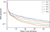 |
Fig. 1 RMS as a function of major loop iteration for M31 obtained with Momentum-CLEAN with different values for μ. |
5.5 Amount of momentum memory
We demonstrated in the previous subsections that the classical CLEAN approach can be accelerated in some scenarios by adding momentum in the subtraction of the residuals or by orthogonalizing the search directions. In fact, referring back to the algorithm presented in Algorithm 6, the memory of the momentum of the previous residual update has one free parameter associated with it: the amount of momentum carried to the next gradient update step μ. The parameter μ shares some similarities with the classical minor loop gain It regulates the step-size of the CLEANing procedure. However, μ is not equivalent to the loop gain, since μ affects the step-size of the major loop, while the traditional loop gain (which needs to be specified for Momentum-CLEAN as well) affects the step-size of the minor loop. The most straightforward illustration of the effect of momentum memory (regulated by μ) in the traditional picture would be a loop gain that varies pixel by pixel in the image, i.e., we allow for steeper component subtraction in regions that have been found to carry significant emission in earlier iterations of the minor loop.
In this subsection, we use the reconstruction of M31 to study the impact of this parameter in the reconstructions. First, we would like to mention that it is anticipated that 0 ≤ μ ≤ 1. μ ≤ 0 would rescind numerical operations done in the previous step. μ ≥ 1 would overdo the correction done in previous steps and lead to pixels that switch between positive and negative values between iterations. In Fig. 1, we show the norm of the residual as a function of the major loop iteration for the different values of μ for M31. We see the best performance at μ = 0.7, close to the value μ = 0.5 chosen in the previous subsection. The performance worsens again for higher values. Moreover, after closer inspection of the red and pink lines (μ = 0.7 and μ = 0.9), the convergence curve shows an oscillatory behavior, where the reconstruction even worsens during some iterations. The same effect is visible in Fig. B.15 for Cygnus A. We attribute this oscillating behavior to the consequence of switching pixels (i.e., some pixels get overcleaned) when we add too much momentum as mentioned above.
6 Conclusions
In this manuscript, we examined the classical Cotton–Schwab CLEAN cycle. Despite the numerous alternative methods proposed over the years, CLEAN remains the de facto standard, primarily due to its robustness and computational efficiency. We offered a novel perspective on the algorithm by interpreting it as a Newton minimization technique. Although this interpretation does not constitute a mathematical equivalence, since several key aspects of the CLEAN algorithm, such as its matching pursuit nature, are not captured in this formulation, and the fundamental assumptions of Newton’s method are violated, this analogy serves as an illustrative framework.
In particular, we demonstrated that the division of CLEAN into major and minor loops can be understood in terms of the individual steps involved in computing the gradient (major loop) and inverting the Hessian (minor loop). Building on this analogy, we proposed a method for identifying new CLEAN variants by the inverse direction of arguments: we began with promising minimization algorithms and expressed them in terms of the robust and numerically efficient major and minor loop iterations by replacing the gradient evolution with the major loop and the inversion of the Hessian with the minor loop. We applied this framework to several minimization algorithms, including implicit gradient descent, CG descent (applied to the normal equation), and heavy-ball (Nesterov) acceleration techniques.
It is important to note that the methodology presented here could, in principle, be extended to a broader range of algorithms with relative ease. The chosen algorithms are not meant to represent a comprehensive list, but rather a set of examples to demonstrate the approach. Additionally, we acknowledge that much of the ongoing research into novel minimization techniques is focused on the development of quasi-Newton and frozen Newton methods, which are unlikely to yield significant improvements in the context of the scope of this manuscript, given that the Hessian is typically known in this domain, and we explicitly aim to apply it here through the minor loop, rather than approximate.
We benchmarked two variants of CLEAN: CG-CLEAN (conjugate gradients interpreted as CLEAN) and Momentum-CLEAN (heavy-ball momentum acceleration applied to CLEAN), against the traditional CLEAN algorithm using multiple test observations. We applied a hierarchically more challenging validation ladder to our procedures, consisting of data from the CASA tutorial on 3C391, synthetic and real narrowband data, and spectral and VLBI data reduction. We observe in all of these examples that CG-CLEAN produces smaller residuals than CLEAN in fewer iterations, obtains compatible or even better reconstructions than CLEAN, and requires fewer major loop iterations, which drives data processing costs. We found similar trends for Momentum-CLEAN in some of the test data. We interpret these findings as indicating that CG-CLEAN achieves significantly faster convergence and requires fewer major loop iterations. Additionally, CG-CLEAN cleans to deeper levels than the original CLEAN, providing improvements in dynamic range that are comparable to, or even exceed, those offered by state-of-the-art minor loop algorithms such as Asp-CLEAN over traditional MS-CLEAN. The best performance is achieved by combining the CG-CLEAN framework in the major loop with Asp-CLEAN operating in the minor loop, allowing the algorithm to reach the noise level after just a few major loop iterations. The claim of faster convergence toward an agreed-on final model is supported by an analysis on synthetic data and a comparison to the ground truth where CG-CLEAN shows higher and faster rising PSNR than traditional techniques. These improvements are realized with only a minimal increase in computational cost and in a framework that can be straightforwardly expanded to more challenging scenarios, including VLBI, wideband, wide field, and mosaicking by reusing the robust implementations already available through CASA. We tested the first two regimes as an example and report the same degree of acceleration.
This work contributes to efforts aimed at scaling data processing techniques for the large data volumes expected from next-generation radio interferometers, such as ngVLA, SKA, and DSA2000. Given that gridding constitutes the primary computational cost for these arrays, any approach that reduces the number of major loop iterations is highly valuable. While the long-term future of data processing may not lie with CLEAN but rather with a variety of more sophisticated imaging procedures already proposed and under development, short- and midterm pipelines can benefit from how straightforwardly CG-CLEAN builds upon existing pipelines. Moreover, the choice of algorithms for future arrays also necessitates the further development of CLEAN methods, at least as a benchmark for the limits of traditional radio interferometric imaging.
Finally, we emphasize that the algorithms discussed in this manuscript are conceptually straightforward. They are built upon robust principles and existing software foundations. As a result, adapting these algorithms into state-of-the-art data processing software should involve minimal challenges.
Acknowledgements
The implementation of this work was performed in the software package CASA (CASA Team 2022). In its earlier development stage of this manuscript, we however made use of software tools providing less monolithic, more modular and simple low-level access to radio-astronomic data. In particular, we would like to acknowledge LibRA5, and MrBeam6 (Müller & Lobanov 2022; Müller et al. 2024). Special thanks goes to Preshanth Jagganathan for his support with the installation and handling of LibRA. This research was supported through the Jansky fellowship program of the National Radio Astronomy Observatory. NRAO is a facility of the National Science Foundation operated under cooperative agreement by Associated Universities, Inc. Furthermore, H.M. acknowledges support by the M2FINDERS project which has received funding from the European Research Council (ERC) under the European Union’s Horizon 2020 Research and Innovation Program (grant agreement No. 101018682).
References
- Aghabiglou, A., Chu, C. S., Dabbech, A., & Wiaux, Y. 2024, ApJS, 273, 3 [NASA ADS] [CrossRef] [Google Scholar]
- Akiyama, K., Kuramochi, K., Ikeda, S., et al. 2017, ApJ, 838, 1 [NASA ADS] [CrossRef] [Google Scholar]
- Arras, P., Bester, H. L., Perley, R. A., et al. 2021, A&A, 646, A84 [NASA ADS] [CrossRef] [EDP Sciences] [Google Scholar]
- Bester, H. L., Kenyon, J. S., Repetti, A., et al. 2026, Astron. Comput., 54, 100996 [Google Scholar]
- Bhatnagar, S., & Cornwell, T. J. 2004, A&A, 426, 747 [NASA ADS] [CrossRef] [EDP Sciences] [Google Scholar]
- Bhatnagar, S., Hirart, R., & Pokorny, M. 2021, Size-of-Computing Estimates for ngVLA Synthesis Imaging, NRAO-The ngVLA Memo Series: Computing Memos [Google Scholar]
- Bhatnagar, S., Madsen, F., & Robnett, J. 2022, Baseline HPG runtime performance for imaging, NRAO-The ngVLA Memo Series: Computing Memos [Google Scholar]
- Bhatnagar, S., Rau, U., Hsieh, M., Kern, J., & Xue, R. 2025, AJ, 170, 246 [Google Scholar]
- Briggs, D. S. 1995, PhD thesis, New Mexico Institute of Mining and Technology [Google Scholar]
- Broderick, A. E., Gold, R., Karami, M., et al. 2020, ApJ, 897, 139 [Google Scholar]
- Carpenter, J. M., Brogan, C. L., Iono, D., & Mroczkowski, T. 2022, arXiv e-prints [arXiv:2211.00195] [Google Scholar]
- CASA Team (Bean, B., et al.) 2022, PASP, 134, 114501 [NASA ADS] [CrossRef] [Google Scholar]
- Chael, A. A., Johnson, M. D., Bouman, K. L., et al. 2018, ApJ, 857, 23 [Google Scholar]
- Connor, L., Bouman, K. L., Ravi, V., & Hallinan, G. 2022, MNRAS, 514, 2614 [NASA ADS] [CrossRef] [Google Scholar]
- Cornwell, T. J. 2008, IEEE J. Sel. Top. Signal Process., 2, 793 [Google Scholar]
- Cornwell, T. J., & Evans, K. F. 1985, A&A, 143, 77 [NASA ADS] [Google Scholar]
- Dabbech, A., Repetti, A., Perley, R. A., Smirnov, O. M., & Wiaux, Y. 2021, MNRAS, 506, 4855 [NASA ADS] [CrossRef] [Google Scholar]
- Dabbech, A., Aghabiglou, A., Chu, C. S., & Wiaux, Y. 2024, ApJ, 966, L34 [NASA ADS] [CrossRef] [Google Scholar]
- Dewdney, P. E., Hall, P. J., Schilizzi, R. T., & Lazio, T. J. L. W. 2009, IEEE Proc., 97, 1482 [Google Scholar]
- Event Horizon Telescope Collaboration (Akiyama, K., et al.) 2019, ApJ, 875, L4 [Google Scholar]
- Event Horizon Telescope Collaboration (Akiyama, K., et al.) 2021, ApJ, 910, 48 [CrossRef] [Google Scholar]
- Event Horizon Telescope Collaboration (Akiyama, K., et al.) 2022, ApJ, 930, L14 [NASA ADS] [CrossRef] [Google Scholar]
- Event Horizon Telescope Collaboration (Akiyama, K., et al.) 2024, ApJ, 964, L25 [NASA ADS] [CrossRef] [Google Scholar]
- Fletcher, R., & Reeves, C. M. 1964, Comput. J., 7, 149 [Google Scholar]
- Garsden, H., Girard, J. N., Starck, J. L., et al. 2015, A&A, 575, A90 [CrossRef] [EDP Sciences] [Google Scholar]
- Gheller, C., & Vazza, F. 2022, MNRAS, 509, 990 [Google Scholar]
- Hallinan, G., Ravi, V., Weinreb, S., et al. 2019, in Bulletin of the American Astronomical Society, 51, 255 [Google Scholar]
- Hamaker, J. P., Bregman, J. D., & Sault, R. J. 1996, A&AS, 117, 137 [NASA ADS] [Google Scholar]
- Högbom, J. A. 1974, A&AS, 15, 417 [Google Scholar]
- Hsieh, G., & Bhatnagar, S. 2021, Efficient Adaptive-Scale CLEAN Deconvolution in CASA for Radio Interferometric Images, NRAO-ARDG Memo Series [Google Scholar]
- Hsieh, G., Bhatnagar, S., Hiriart, R., & Pokorny, M. 2022a, Recommended Developments Necessary for Applying (W)Asp Deconvolution Algorithms to ngVLA, NRAO-ARDG Memo Series [Google Scholar]
- Hsieh, G., Rau, U., & Bhatnagar. 2022b, An Adaptive-Scale Multi-Frequency Deconvolution of Interferometric Images, NRAO-ARDG Memo Series [Google Scholar]
- Hunter, T. R., Indebetouw, R., Brogan, C. L., et al. 2023, PASP, 135, 074501 [NASA ADS] [CrossRef] [Google Scholar]
- Jarret, A., Kashani, S., Rué-Queralt, J., et al. 2025, A&A, 693, A225 [NASA ADS] [CrossRef] [EDP Sciences] [Google Scholar]
- Junklewitz, H., Bell, M. R., Selig, M., & Enßlin, T. A. 2016, A&A, 586, A76 [NASA ADS] [CrossRef] [EDP Sciences] [Google Scholar]
- Kepley, A., Madsen, F., Robnet, J., & Rowe, K. 2023, Imaging Unmitigated ALMA Cubes, nAASC memo series [Google Scholar]
- Lister, M. L., Aller, M. F., Aller, H. D., et al. 2018, ApJS, 234, 12 [CrossRef] [Google Scholar]
- Lu, R.-S., Asada, K., Krichbaum, T. P., et al. 2023, Nature, 616, 686 [CrossRef] [Google Scholar]
- Müller, H., & Bhatnagar, S. 2025, A&A, 698, A176 [NASA ADS] [CrossRef] [EDP Sciences] [Google Scholar]
- Müller, H., & Lobanov, A. P. 2022, A&A, 666, A137 [NASA ADS] [CrossRef] [EDP Sciences] [Google Scholar]
- Müller, H., & Lobanov, A. P. 2023a, A&A, 673, A151 [NASA ADS] [CrossRef] [EDP Sciences] [Google Scholar]
- Müller, H., & Lobanov, A. P. 2023b, A&A, 672, A26 [NASA ADS] [CrossRef] [EDP Sciences] [Google Scholar]
- Müller, H., Mus, A., & Lobanov, A. 2023, A&A, 675, A60 [NASA ADS] [CrossRef] [EDP Sciences] [Google Scholar]
- Müller, H., Massa, P., Mus, A., Kim, J.-S., & Perracchione, E. 2024, A&A, 684, A47 [NASA ADS] [CrossRef] [EDP Sciences] [Google Scholar]
- Murphy, E. J., Bolatto, A., Chatterjee, S., et al. 2018, in Astronomical Society of the Pacific Conference Series, 517, Science with a Next Generation Very Large Array, ed. E. Murphy, 3 [Google Scholar]
- Mus, A., Müller, H., & Lobanov, A. 2024, A&A, 688, A100 [NASA ADS] [CrossRef] [EDP Sciences] [Google Scholar]
- Nocedal, J., & Wright, S. 2006, Numerical Optimization, Springer Series in Operations Research and Financial Engineering (Springer New York) [Google Scholar]
- Offringa, A. R., & Smirnov, O. 2017, MNRAS, 471, 301 [Google Scholar]
- Offringa, A. R., McKinley, B., Hurley-Walker, N., et al. 2014, MNRAS, 444, 606 [Google Scholar]
- Onose, A., Dabbech, A., & Wiaux, Y. 2017, MNRAS, 469, 938 [NASA ADS] [CrossRef] [Google Scholar]
- Rau, U., & Cornwell, T. J. 2011, A&A, 532, A71 [NASA ADS] [CrossRef] [EDP Sciences] [Google Scholar]
- Roth, J., Arras, P., Reinecke, M., et al. 2023, A&A, 678, A177 [NASA ADS] [CrossRef] [EDP Sciences] [Google Scholar]
- Roth, J., Frank, P., Bester, H. L., et al. 2024, A&A, 690, A387 [NASA ADS] [CrossRef] [EDP Sciences] [Google Scholar]
- Sandstrom, K. M., Chastenet, J., Sutter, J., et al. 2023a, ApJ, 944, L7 [NASA ADS] [CrossRef] [Google Scholar]
- Sandstrom, K. M., Koch, E. W., Leroy, A. K., et al. 2023b, ApJ, 944, L8 [NASA ADS] [CrossRef] [Google Scholar]
- Schwab, F. R. 1984, AJ, 89, 1076 [NASA ADS] [CrossRef] [Google Scholar]
- Selina, R. J., Murphy, E. J., McKinnon, M., et al. 2018, in Astronomical Society of the Pacific Conference Series, 517, Science with a Next Generation Very Large Array, ed. E. Murphy, 15 [Google Scholar]
- Smirnov, O. M. 2011, A&A, 527, A106 [NASA ADS] [CrossRef] [EDP Sciences] [Google Scholar]
- Starck, J.-L., Bijaoui, A., Lopez, B., & Perrier, C. 1994, A&A, 283, 349 [NASA ADS] [Google Scholar]
- Sun, H., Bouman, K. L., Tiede, P., et al. 2022, ApJ, 932, 99 [NASA ADS] [CrossRef] [Google Scholar]
- Thompson, A. R., Moran, J. M., & Swenson, George W., J. 2017, Interferometry and Synthesis in Radio Astronomy, 3rd edn. [Google Scholar]
- Wiaux, Y., Jacques, L., Puy, G., Scaife, A. M. M., & Vandergheynst, P. 2009, MNRAS, 395, 1733 [NASA ADS] [CrossRef] [Google Scholar]
Self-calibrated data shared in private communication by Rick Perley, Program Code: 14B-336.
Program code: VLA-23B-025, PI: Karin Sandstrom.
August 19, 2018.
Appendix A Proof of orthogonality
We now show by induction on the number of major loop iterations k that the search directions are orthogonal to each other with respect to the beam, i.e., ![Mathematical equation: $\[p_{i}^{+} B p_{j}=0\]$](/articles/aa/full_html/2026/02/aa55356-25/aa55356-25-eq55.png) for indices i ≠ j and
for indices i ≠ j and ![Mathematical equation: $\[I_{k}^{+} p_{i}=0\]$](/articles/aa/full_html/2026/02/aa55356-25/aa55356-25-eq56.png) for i < k. For the induction beginning, we compute
for i < k. For the induction beginning, we compute ![Mathematical equation: $\[I_{1}^{+} p_{0}\]$](/articles/aa/full_html/2026/02/aa55356-25/aa55356-25-eq57.png) . We obtain
. We obtain
![Mathematical equation: $\[I_1^{+} p_0=I_0^{+} p_0-\alpha_0 p_0^{+} B p_0=0,\]$](/articles/aa/full_html/2026/02/aa55356-25/aa55356-25-eq58.png)
by the definition of α0. Moreover, we have
![Mathematical equation: $\[p_1^{+} B p_0=z_1^{+} B p_0+\beta_0 p_0^{+} B p_0=0,\]$](/articles/aa/full_html/2026/02/aa55356-25/aa55356-25-eq59.png)
by the definition of β0. To follow, we consider the induction step, k → k + 1. For i < k + 1,
![Mathematical equation: $\[I_{k+1}^{+} p_i=I_k^{+} p_i-\alpha_k p_k^{+} B p_i.\]$](/articles/aa/full_html/2026/02/aa55356-25/aa55356-25-eq60.png)
If i = k, then the right-hand side vanishes due to the definition of αk. If i < k, then both terms vanish by the induction assumption. Similarly, we have
![Mathematical equation: $\[p_{k+1}^{+} B p_i=z_{k+1}^{+} B p_i+\beta_k p_k^{+} B p_i.\]$](/articles/aa/full_html/2026/02/aa55356-25/aa55356-25-eq61.png)
If i = k, then the right-hand side vanishes due to definition of βk. If i < k, the second term on the right-hand side vanishes by the induction assumption. For the first term, note that Bzk+1 ≈ Ik+1, so the first term vanishes as well.
We would like to note that these properties only hold exactly in the absence of grid and calibration errors. In practice however, one would typically need to stop the minor loop earlier based on manually enforced stopping criteria before the noise-level is reached and potentially manipulate the dataset itself (e.g., self-calibration or flagging). As a consequence the relation Bzk = Ik holds only approximately. Moreover, the relation Ik+1 = Ik − αkBpk also holds only approximately in the presence of gridding errors. Both are needed to ensure exact orthogonality of the search directions pk. Application in practice may benefit from restarting CG iterations. Nevertheless, the arguments listed above show that at least directly following search directions pk, pk+1 are orthogonal on each other.
We note that the necessity to restart the CG iterations is not conceptually different from the wide-spread application of the algorithm outside the interferometry context. It is a fairly common scenario due to departures from orthogonality, which accumulate due to numerical errors. However, specifically in radio interferometry, such additional sources of errors as gridding and calibration exist.
There are two trivial corollaries to these identities. Since zk ∈ span[pk−1, pk], we also have ![Mathematical equation: $\[I_{k}^{+} z_{i}=0\]$](/articles/aa/full_html/2026/02/aa55356-25/aa55356-25-eq62.png) for all i < k. Similarly, we get for
for all i < k. Similarly, we get for ![Mathematical equation: $\[i<k, I_{i}^{+} z_{k}=z_{i}^{+} B z_{k}=I_{k}^{+} z_{i}=0\]$](/articles/aa/full_html/2026/02/aa55356-25/aa55356-25-eq63.png) . We make use of these identities below.
. We make use of these identities below.
Note that for k ≥ 1:
![Mathematical equation: $\[I_k^{+} p_k=I_k^{+} z_k+\beta_{k-1} I_k^{+} p_{k-1}=I_k^{+} z_k.\]$](/articles/aa/full_html/2026/02/aa55356-25/aa55356-25-eq64.png)
Hence, we also get:
![Mathematical equation: $\[\alpha_k=\frac{I_k^{res,+} z_k}{p_k^{+} B p_k}.\]$](/articles/aa/full_html/2026/02/aa55356-25/aa55356-25-eq65.png) (A.1)
(A.1)
Moreover, it is:
![Mathematical equation: $\[\alpha_k z_{k+1}^{+} B p_k=-z_{k+1}^{+} I_{k+1}.\]$](/articles/aa/full_html/2026/02/aa55356-25/aa55356-25-eq66.png)
Together, we get:
![Mathematical equation: $\[\beta_k=\frac{I_{k+1}^{+} z_{k+1}}{I_k^{+} z_k}\]$](/articles/aa/full_html/2026/02/aa55356-25/aa55356-25-eq67.png) (A.2)
(A.2)
Eq. (A.1) and Eq. (A.2) define equivalent, alternative definitions for the step-size parameters α and β.
Appendix B Figures of our reconstruction results
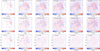 |
Fig. B.1 Residual as a function of increasing major loop iterations (from left to right) for 3C391, for CLEAN (top row), Momentum CLEAN (middle row), and CG-CLEAN (bottom row). |
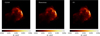 |
Fig. B.2 The recovered image of 3C391 with MS-CLEAN (left panel), Momentum-CLEAN (middle panel), and CG-CLEAN (right panel). |
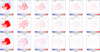 |
Fig. B.3 Difference between the current model and the final model (after the last major loop iteration) as a function of increasing major loop iterations (from left to right) for 3C391 for CLEAN (top row), Momentum CLEAN (middle row), and CG-CLEAN (bottom row). |
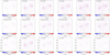 |
Fig. B.4 Residual as a function of increasing major loop iterations (from left to right) for synthetic Cygnus A data for CLEAN (top row), Momentum CLEAN (middle row), and CG-CLEAN (bottom row). |
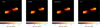 |
Fig. B.5 The ground truth image (left panel) and the recovered images of synthetic Cygnus A data using MS-CLEAN (second panel), Momentum-CLEAN (third panel), and CG-CLEAN (right panel). |
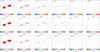 |
Fig. B.6 Difference between the current model and the final model (after the last major loop iteration) as a function of increasing major loop iterations (from left to right) for synthetic ENZO simulation data for CLEAN (top row), Momentum CLEAN (middle row), and CG-CLEAN (bottom row). |
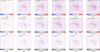 |
Fig. B.7 Residual as a function of increasing major loop iterations (from left to right) for synthetic ENZO simulation data for CLEAN (top row), Momentum CLEAN (middle row), and CG-CLEAN (bottom row). |
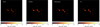 |
Fig. B.8 Ground truth image (left panel) and recovered images of synthetic ENZO simulation data using MS-CLEAN (second panel), Momentum-CLEAN (third panel), and CG-CLEAN (right panel). |
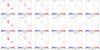 |
Fig. B.9 Difference between the current model and the final model (after the last major loop iteration) as a function of increasing major loop iterations (from left to right) for synthetic Cygnus A data for CLEAN (top row), Momentum CLEAN (middle row), and CG-CLEAN (bottom row). |
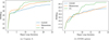 |
Fig. B.10 PSNR of the reconstructions as a function of major loop iteration for synthetic data of Cygnus A (left panel) and a simulated galaxy from the ENZO simulation suite (right panel). |
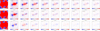 |
Fig. B.11 Residual as a function of increasing major loop iterations (from left to right) for Cygnus A. Top: CLEAN. Middle: Momentum CLEAN. Bottom: CG-CLEAN. |
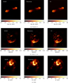 |
Fig. B.14 Recovered models with CLEAN (left column), Momentum CLEAN (middle column), and CG-CLEAN (right column) for Cygnus A (first row), G055.7+3.4 (middle row), and M31 (bottom row). |
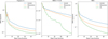 |
Fig. B.15 Norm of the residual as a function of major loop iteration for CLEAN (blue), Momentum CLEAN (orange), and CG-CLEAN (green). Left to right: Results for Cygnus A, G055.7+3.4, and M31. |
 |
Fig. B.16 Residual as a function of major loop iteration for Cygnus A. Here, we compare traditional CLEAN with CG-CLEAN in two different flavors for the minor loop. First row: Cotton–Schwab major cycles with MS-CLEAN in the minor loop. Second row: Cotton–Schwab major cycles with Asp-CLEAN in the minor loop. Third row: CG-CLEAN with MS-CLEAN in the minor loop. Fourth row: CG-CLEAN with Asp-CLEAN in the minor loop. |
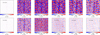 |
Fig. B.19 Residual as a function of increasing major loop iterations (from left to right) for MOJAVE observations of 3C120 for CLEAN (top row) and CG-CLEAN (bottom row). |
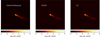 |
Fig. B.20 Stacked image of 3C120 (stacked from 30 years of data-taking observations, left panel) and our reconstructions of a single epoch with MS-CLEAN (middle panel), and CG-CLEAN (right panel). |
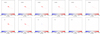 |
Fig. B.21 Difference between the current model and the final model (after the last major loop iteration) as a function of increasing major loop iterations (from left to right) for MOJAVE single-epoch observations of 3C120 for CLEAN (top row) and CG-CLEAN (bottom row). |
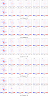 |
Fig. B.22 Residual as a function of increasing major loop iterations (from left to right) for NGC 628 with the VLA for CLEAN (top rows of every sub-figure) and CG-CLEAN (bottom rows of every sub-figure). The sub-figures show different spectral channels. |
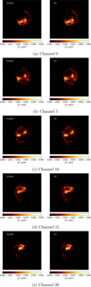 |
Fig. B.23 Recovered models with CLEAN (left column) and CG-CLEAN (right column) for NGC 628 observations with the VLA. The sub-figures show different spectral channels. |
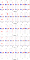 |
Fig. B.24 Difference between the current model and the final model (after the last major loop iteration) as a function of increasing major loop iterations (from left to right) for NGC 628 with the VLA for CLEAN (top rows in every sub-figure) and CG-CLEAN (bottom row in every sub-figure). The sub-figures show different spectral channels. |
All Figures
|
Fig. 1 RMS as a function of major loop iteration for M31 obtained with Momentum-CLEAN with different values for μ. |
| In the text | |
|
Fig. B.1 Residual as a function of increasing major loop iterations (from left to right) for 3C391, for CLEAN (top row), Momentum CLEAN (middle row), and CG-CLEAN (bottom row). |
| In the text | |
|
Fig. B.2 The recovered image of 3C391 with MS-CLEAN (left panel), Momentum-CLEAN (middle panel), and CG-CLEAN (right panel). |
| In the text | |
|
Fig. B.3 Difference between the current model and the final model (after the last major loop iteration) as a function of increasing major loop iterations (from left to right) for 3C391 for CLEAN (top row), Momentum CLEAN (middle row), and CG-CLEAN (bottom row). |
| In the text | |
|
Fig. B.4 Residual as a function of increasing major loop iterations (from left to right) for synthetic Cygnus A data for CLEAN (top row), Momentum CLEAN (middle row), and CG-CLEAN (bottom row). |
| In the text | |
|
Fig. B.5 The ground truth image (left panel) and the recovered images of synthetic Cygnus A data using MS-CLEAN (second panel), Momentum-CLEAN (third panel), and CG-CLEAN (right panel). |
| In the text | |
|
Fig. B.6 Difference between the current model and the final model (after the last major loop iteration) as a function of increasing major loop iterations (from left to right) for synthetic ENZO simulation data for CLEAN (top row), Momentum CLEAN (middle row), and CG-CLEAN (bottom row). |
| In the text | |
|
Fig. B.7 Residual as a function of increasing major loop iterations (from left to right) for synthetic ENZO simulation data for CLEAN (top row), Momentum CLEAN (middle row), and CG-CLEAN (bottom row). |
| In the text | |
|
Fig. B.8 Ground truth image (left panel) and recovered images of synthetic ENZO simulation data using MS-CLEAN (second panel), Momentum-CLEAN (third panel), and CG-CLEAN (right panel). |
| In the text | |
|
Fig. B.9 Difference between the current model and the final model (after the last major loop iteration) as a function of increasing major loop iterations (from left to right) for synthetic Cygnus A data for CLEAN (top row), Momentum CLEAN (middle row), and CG-CLEAN (bottom row). |
| In the text | |
|
Fig. B.10 PSNR of the reconstructions as a function of major loop iteration for synthetic data of Cygnus A (left panel) and a simulated galaxy from the ENZO simulation suite (right panel). |
| In the text | |
|
Fig. B.11 Residual as a function of increasing major loop iterations (from left to right) for Cygnus A. Top: CLEAN. Middle: Momentum CLEAN. Bottom: CG-CLEAN. |
| In the text | |
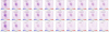 |
Fig. B.12 Same as Fig. B.11, but for G055.7+3.4. |
| In the text | |
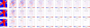 |
Fig. B.13 Same as Fig. B.11, but for M31. |
| In the text | |
|
Fig. B.14 Recovered models with CLEAN (left column), Momentum CLEAN (middle column), and CG-CLEAN (right column) for Cygnus A (first row), G055.7+3.4 (middle row), and M31 (bottom row). |
| In the text | |
|
Fig. B.15 Norm of the residual as a function of major loop iteration for CLEAN (blue), Momentum CLEAN (orange), and CG-CLEAN (green). Left to right: Results for Cygnus A, G055.7+3.4, and M31. |
| In the text | |
|
Fig. B.16 Residual as a function of major loop iteration for Cygnus A. Here, we compare traditional CLEAN with CG-CLEAN in two different flavors for the minor loop. First row: Cotton–Schwab major cycles with MS-CLEAN in the minor loop. Second row: Cotton–Schwab major cycles with Asp-CLEAN in the minor loop. Third row: CG-CLEAN with MS-CLEAN in the minor loop. Fourth row: CG-CLEAN with Asp-CLEAN in the minor loop. |
| In the text | |
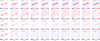 |
Fig. B.17 Same as Fig. B.16, but for G055.7+3.4. |
| In the text | |
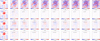 |
Fig. B.18 Same as Fig. B.16, but for M31. |
| In the text | |
|
Fig. B.19 Residual as a function of increasing major loop iterations (from left to right) for MOJAVE observations of 3C120 for CLEAN (top row) and CG-CLEAN (bottom row). |
| In the text | |
|
Fig. B.20 Stacked image of 3C120 (stacked from 30 years of data-taking observations, left panel) and our reconstructions of a single epoch with MS-CLEAN (middle panel), and CG-CLEAN (right panel). |
| In the text | |
|
Fig. B.21 Difference between the current model and the final model (after the last major loop iteration) as a function of increasing major loop iterations (from left to right) for MOJAVE single-epoch observations of 3C120 for CLEAN (top row) and CG-CLEAN (bottom row). |
| In the text | |
|
Fig. B.22 Residual as a function of increasing major loop iterations (from left to right) for NGC 628 with the VLA for CLEAN (top rows of every sub-figure) and CG-CLEAN (bottom rows of every sub-figure). The sub-figures show different spectral channels. |
| In the text | |
|
Fig. B.23 Recovered models with CLEAN (left column) and CG-CLEAN (right column) for NGC 628 observations with the VLA. The sub-figures show different spectral channels. |
| In the text | |
|
Fig. B.24 Difference between the current model and the final model (after the last major loop iteration) as a function of increasing major loop iterations (from left to right) for NGC 628 with the VLA for CLEAN (top rows in every sub-figure) and CG-CLEAN (bottom row in every sub-figure). The sub-figures show different spectral channels. |
| In the text | |
Current usage metrics show cumulative count of Article Views (full-text article views including HTML views, PDF and ePub downloads, according to the available data) and Abstracts Views on Vision4Press platform.
Data correspond to usage on the plateform after 2015. The current usage metrics is available 48-96 hours after online publication and is updated daily on week days.
Initial download of the metrics may take a while.