| Issue |
A&A
Volume 706, February 2026
|
|
|---|---|---|
| Article Number | A82 | |
| Number of page(s) | 17 | |
| Section | Interstellar and circumstellar matter | |
| DOI | https://doi.org/10.1051/0004-6361/202555671 | |
| Published online | 04 February 2026 | |
Interacting supernovae and where to find them
1
Institute of Physics and Astronomy, University of Potsdam,
14476
Potsdam-Golm,
Germany
2
School of Physical Sciences and Centre for Astrophysics & Relativity, Dublin City University,
Glasnevin,
D09 W6Y4,
Ireland
3
Astronomy & Astrophysics Section, School of Cosmic Physics, Dublin Institute for Advanced Studies, DIAS Dunsink Observatory,
Dublin
D15 XR2R,
Ireland
4
Centro de Investigaciones Energéticas, Medioambientales y Tecnológicas (CIEMAT),
28040
Madrid,
Spain
5
Gran Sasso Science Institute,
Via F.Crispi 7,
67100
L’Aquila,
Italy
6
INFN-Laboratori Nazionali del Gran Sasso,
Via G. Acitelli 22,
Assergi (AQ),
Italy
7
Centre for Space Research, North-West University,
2520
Potchefstroom,
South Africa
8
Astronomical Observatory of Ivan Franko National University of Lviv,
Kyryla i Methodia 8,
79005
Lviv,
Ukraine
9
ASTRON – Netherlands Institute for Radio Astronomy,
Oude Hoogeveensedijk 4,
7991 PD
Dwingeloo,
The Netherlands
★ Corresponding author: This email address is being protected from spambots. You need JavaScript enabled to view it.
Received:
26
May
2025
Accepted:
19
October
2025
Abstract
Context. The early interaction of supernova blast waves with circumstellar material has the potential to accelerate particles to petaelectronvolt energies, although this has not yet been detected. Current models for this interaction assume that the blast wave expands into a smooth freely expanding stellar wind, although multiwavelength observations of many supernovae do not support this assumption.
Aims. We extend previous work by considering blast waves expanding into complex density profiles consisting of smooth winds with dense circumstellar shells at various distances from the progenitor star. We aim to predict the gamma-ray and multiwavelength signatures of circumstellar interaction.
Methods. We used the code PION to model the circumstellar medium around luminous blue variables including a brief episode of enhanced mass-loss and to simulate the formation of photoionization-confined shells around red supergiants. Consequently, we used the time-dependent acceleration code RATPaC to study the acceleration of cosmic rays in supernovae expanding into these media and to evaluate the emitted radiation (both thermal and nonthermal) across the whole electromagnetic spectrum.
Results. We find that the interaction with the circumstellar shells can significantly boost the gamma-ray emission of a remnant, with the emission peaking weeks to years after the explosion when γγabsorption has reduced to negligible levels. The peak luminosity for Type IIP and Type IIn remnants can exceed the luminosity expected for smooth winds by several orders of magnitude. For Type IIP explosions, the light-curve peak is only reached years after the explosion, when the blast wave reaches the circumstellar shell. We evaluated the multiwavelength signatures expected from the interaction of the blast wave with a dense circumstellar shell from radio to optical and thermal X-rays.
Conclusions. High-cadence optical surveys and continuous monitoring of nearby supernovae in radio and millimeter wavelengths are the best-suited strategies for identifying targets. They should be followed-up by gamma-ray observatories. We predict that gamma-rays from interaction with dense circumstellar shells may be detectable out to a few megaparsec for late interaction and out to tens of megaparsec for an early interaction.
Key words: acceleration of particles / shock waves / methods: numerical / ISM: supernova remnants / gamma rays: general
© The Authors 2026
 Open Access article, published by EDP Sciences, under the terms of the Creative Commons Attribution License (https://creativecommons.org/licenses/by/4.0), which permits unrestricted use, distribution, and reproduction in any medium, provided the original work is properly cited.
This article is published in open access under the Subscribe to Open model. This email address is being protected from spambots. You need JavaScript enabled to view it. to support open access publication.
1 Introduction
For almost one hundred years, supernova remnants (SNRs) have been extensively studied and discussed as potential major sources of Galactic cosmic rays (CRs) with energies up to the knee feature in the CR spectrum at a few petaelectronvolt (PeV) (see e.g. Baade & Zwicky 1934; Blandford & Eichler 1987). Advances in gamma-ray observations of historical SNRs such as Tycho and Casiopeia A, which initially were expected to be effective particle accelerators, show cutoff energies considerably below 1 PeV (Abeysekara et al. 2020). Based on theoretical considerations, young remnants a few years after the supernova (SN) explosion moved into focus, and current research investigates whether these objects might be able to reach PeV energies (Marcowith et al. 2018; Cristofari et al. 2020a,b; Inoue et al. 2021; Brose et al. 2022; Diesing 2023; Brose et al. 2025; Sushch et al. 2025).
A detection of the gamma-ray signatures associated with efficient particle acceleration would be essential to answering this question, but only radio emission shows clear evidence for non-thermal emission from relativistic particles so far (Bietenholz et al. 2021), although Dwarkadas (2025) argued that the X-ray luminosity of some Type Ib/c and IIP SNe are too high to be explained by thermal emission and that a nonthermal component should therefore be present. Theoretically, most of the promising scenarios require an exceptionally dense circumstellar medium (CSM) (Bell et al. 2013), and phenomenological models suggest that these events might be detectable out to distances of several hundred megaparsec (Murase et al. 2011, 2014). Work that also accounted for the γγabsorption of the gamma-rays by interaction with photons from the SN photosphere obtained considerably lower horizon estimates that were at megaparsec scales (Tatischeff 2009). Many works followed and estimated similar detection horizons for these young objects based on more detailed descriptions of the acceleration and γγabsorption (Cristofari et al. 2020b, 2022; Brose et al. 2022, and references therin).
Despite intensive experimental effort, a detection of gamma-rays from a very young SNR has yet to be reported. There are indications of a transient γ-ray signal in data of the Large Area Telescope on board the Fermi satellite (Fermi-LAT) overlapping with the positions of SN 2004dj, a Type IIP explosion (Xi et al. 2020), and SN iPTF14hls (Yuan et al. 2018), at distances of 3.5 and 156 Mpc, respectively. Additionally, two more SN candidates were found in a transient search throughout the Fermi-LAT archive (Prokhorov et al. 2021). Fermi-LAT upper limits toward the nearby SN 2023ixf1 were used to constrain the acceleration efficiency to values <1% (Martí-Devesa et al. 2024). Similarly, only Fermi-LAT upper limits were reported for the nearby SN 2024ggi (Marti-Devesa & Fermi-LAT Collaboration 2024). A systematic search for gamma-rays associated with Type IIn SNe (the subclass with the highest known CSM densities) showed no signal for individual SNe or the combined sample of SNe (Ackermann et al. 2015). Despite dedicated observing campaigns and searches, no detection of very high-energy (VHE) gamma-ray emission was reported from any core-collapse SNe either (H.E.S.S. Collaboration 2019; Abdalla et al. 2021).
In contrast to the lack of an SNe detection, novae with far lower energies are now established as GeV (Ackermann et al. 2014) and TeV (H.E.S.S. Collaboration 2022; Acciari et al. 2022) sources of gamma-rays, implying efficient particle acceleration in the first few days after the explosion. The physical processes and conditions of blast-wave propagation in core-collapse SNe are very similar to recurrent novae in many respects when the energy and ejecta mass are scaled up by a few orders of magnitude. This reinforces the consensus that GeV and TeV emission will be detected from SNe if they explode sufficiently close to Earth.
A shortcoming of all the theoretical work cited above is that the progenitor star is assumed to have had a constant mass-loss rate on the relevant timescales prior to the explosion, resulting in a smooth wind-profile where the gas density is ρ(r) ∝ r−2 as a function of distance, r, from the star. From the point of view of stellar evolution, this is a strong assumption, and it might not be valid in many cases. In the late evolutionary stages, massive stars may undergo rapid changes in radius, with associated changes in mass-loss rate and wind speed (e.g. Langer 2012). Evidence is increasing that the mass loss of Type IIP explosions in particular is higher immediately before the explosion (Jacobson-Galán et al. 2022, 2025). Recent studies of radio emission from core-collapse SNe (Matsuoka et al. 2025) also support the conclusion that a region of very dense CSM exists around many SN progenitors. This further challenges the theoretical models described above.
The matter is further complicated by luminous blue variable stars (LBVs), which are the likely progenitors of Type IIn SNe. In their giant eruptions, material of a few solar masses is ejected on the timescale of a year, and it expands with ≈100 km s−1. The most famous example is η Carinae (Smith 2014). Red supergiants (RSGs), on the other hand, might feature external photoionization of their wind from nearby hot stars that might shock and partially confine the RSG wind into dense shells with high compression ratios with respect to the freely expanding wind (Mackey et al. 2014). These photoionization-confined shells are thought to have a typical distance of 0.01–1 pc from the RSG, depending on the wind density and on the intensity of the external radiation field.
As a result of the structured nature of the CSM, the SNR blast wave can only interact with the dense CSM with a considerable delay. For example, dense shells at r ≈ 0.01−1 pc trigger late-time circumstellar interaction years after the explosion, as was detected in infrared surveys (Fox et al. 2013). This challenges existing theoretical models and observational strategies: Imaging Air Cherenkov Telescopes (IACTs) usually try to observe SNe within the first weeks after explosion, and Fermi-LAT analysis often focuses on the emission within the first year after the explosion, so that later emission can easily be missed. A notable exception here is the Type IIP SN 2004dj, for which the reported gamma-ray signal appeared ≈5 years after the explosion (Xi et al. 2020). This roughly coincided with the time at which a blast wave would reach the typical location of a photoionization-confined shell. When CSM interactions are common, however, they induce a late-time brightening in gamma-rays that is accompanied by signatures in other wavelengths. It is important to develop trigger strategies for current and next-generation gamma-ray telescopes that take this possibility into account.
We build on our previous publications, Brose et al. (2022, hereafter Paper I) and Brose et al. (2025, hereafter Paper II). In Paper I we studied particle acceleration and nonthermal emission from SNRs associated with explosions of LBV and RSG stars for explosions into smooth 1/r2 density profiles appropriate for stellar winds without variability. There, we developed the revenant descriptions for the emission and absorption processes relevant for these very young SNRs. In Paper II, we studied how the interaction of an SN blast wave with dense shells in Type IIn explosions (associated with LBV progenitors) affects the maximum energy achievable in these cases. We found that the interaction with the dense shells can boost the maximum energy beyond 1 PeV if the interactions occur early enough. This illustrates that a more realistic description of the CSM around massive stars is required.
In this work, we focus on the multiwavelength signatures that arise from the interaction of the blast waves with these dense shells. While Paper II solely focused on LBV progenitors, we additionally consider RSG progenitors in this work, where the dense photoionization-confined shells might not affect the maximum achievable energy, but can significantly alter the multiwavelength light curves.
Section 2 describes the model setup and introduces our assumptions for the density and magnetic field of pre-supernova CSM. We also further discuss the implications of certain aspects of our numeric simulations and the assumptions on which they rely. In Section 3 we describe the emission signatures from gamma-rays to radio and the horizon out to which SN can be detected by current and future observatories, followed by a revised observation strategy (Section 4) based on our findings. Section 5 presents our conclusions.
2 Model setup
The numerical setup of simulations and the basic assumptions and equations that are solved are identical to Paper II. We used the code RATPaC to combine a kinetic treatment of the CRs with a thermal leakage injection model, a fully time-dependent treatment of the magnetic turbulence, and a PLUTO-based hydrodynamic calculation (Telezhinsky et al. 2013; Brose et al. 2016; Mignone et al. 2007). All of the calculations were performed assuming spherical symmetry on a 1D computational grid. The essential ansatz to describe the evolution of the CR distribution is to solve the kinetic diffusion-advection equation for CR-transport (Skilling 1975),
 (1)
where Dr denotes the spatial diffusion coefficient, u is the advective velocity,
(1)
where Dr denotes the spatial diffusion coefficient, u is the advective velocity,  describes the energy losses, and Q is the source of thermal particles.
For a detailed description of the setup, we refer to Paper I and Paper II. We focus on the additional assumptions made for the RSG progenitors here. An in-depth discussion of the assumed microphysics of the self-generated turbulence and their impact on the results can be found in Paper II.
Parameters for the progenitor star winds and initial remnant sizes.
2.1 Circumstellar medium
We considered LBV and RSG progenitors as the most optimistic scenarios for enhanced emission due to interaction with CSM shells. The densest CSM is expected to be formed by LBV eruptions, where the mass-loss rate can reach values as high as 1 M⊙ yr−1 for periods of a few years (Smith 2014). It is slowly becoming evident that RSGs might also have enhanced mass-loss rates of up to 10−2 M⊙ yr−1 a few years prior to explosion (Jacobson-Galán et al. 2022). Moreover, some RSGs may feature dense photoionization-confined shells that can trap up to 35% of the mass that is lost during the RSG phase of stellar evolution (Mackey et al. 2014). While Type IIn SNe that are observationally associated with LBVs constitute only ≈5% of the CCSN rate (Cold & Hjorth 2023), RSGs are the most common SNe progenitors resulting in Type IIP explosions that comprise ≈50% of all CCSNe (Smith et al. 2011). It must be noted, however, that the large majority of SN IIP do not interact with dense circumstellar shells at scales of tens of mpc, and the incidence of these shells is therefore expected to be low.
2.1.1 Modeling the LBV shell
The simplest model for an LBV eruption is to impose a dramatically increased mass-loss rate for a short period of time. We modeled an evolving stellar wind with PION (Mackey et al. 2021) in spherical symmetry by simulating the expansion of a stellar wind in three phases. The mass-loss rate in the first phase was Ṁ = 10−4 M⊙ yr−1 and the terminal wind velocity was v∞ = 100 km s−1 and lasted for 1800 years; the mass-loss rate in the second (outburst) phase was Ṁ = 1 M⊙ yr−1 with a terminal wind velocity of v∞ = 100 km s−1 and lasted for 2 years; and the third phase was the same as the first, but we integrated for 10 000 years. so that the shell expanded to a radius of about 1 parsec. The density structure of the shell was then used to construct the circumstellar shell in the RATPAC simulations, as described below in Section 2.1.3, where some smoothing was applied so that the shock-finding algorithm worked as intended. Examples of the CSM structure can be found in Section 2.1 of Paper II.
2.1.2 Photoionized shells around RSGs
For the photoionization-confined shell model, we considered two different cases to produce a high- and a low-mass CSM shell. For the high-mass shell, we considered an RSG with Ṁ = 10−4 M⊙ yr−1 and v∞ = 15 km s−1. This mass-loss rate is appropriate for the most massive RSGs, such as VY CMa (e.g. Smith et al. 2009). This wind was exposed to an external ionizing flux of Fγ = 1.7 × 10¹² s−1, following the methods presented by Mackey et al. (2014) and Mackey et al. (2015). The system was evolved in spherical symmetry with PION for 200 kyr, during which time, the RSG lost 20 M⊙ through stellar wind. A dense, cold, and thin shell formed at a radius of about 0.03 pc in the wind because of the D-type ionization front that forms in externally photoionized wind. The shock was essentially isothermal, and the compression factor was therefore determined by the minimum obtained temperature, which in this case was about 100 K. At this radius, the wind density is ρ ≈ 2 × 10⁻²⁰ g cm−3, whereas the thin shell was more than 100 times denser. For the low-mass shell, the RSG wind diluted to Ṁ = 2 × 10⁻⁵ M⊙ yr−1 and the ionizing flux to Fγ = 1.7 × 10¹⁰ s−1, which resulted in a CSM shell with a mass lower by about ten times than in the high-mass case. The parameters we used for the two photoionized shells were identical to those used for two calculations in Mackey et al. (2015), who modeled the Hα nebula around the star Wd1-26 in Westerlund 1. The shell properties are given in Table 1, and the density profiles are plotted in Fig. 1. As with the LBV case, the PION density field was used to construct the pre-SN CSM in the RATPaC calculation as described below.
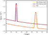 |
Fig. 1 Density profile of the CSM for the two RSG scenarios listed in Table 1. The low mass-loss case creates a more strongly diluted (yellow) shell than the high mass-loss case (purple). The dashed red lines show the density profiles. |
2.1.3 Unified shell model
In Paper II we modeled the CSM density profile for the LBVs alone. Here, we additionally introduce shells with a higher mass following a Gaussian distribution for the RSGs using the same prescription,
 (2)
where Mshell is the shell mass, dshell is the shell thickness, and Rshell is the radial position of the shell. The parameters for the free winds and the corresponding shells are given in Table 1.
(2)
where Mshell is the shell mass, dshell is the shell thickness, and Rshell is the radial position of the shell. The parameters for the free winds and the corresponding shells are given in Table 1.
We obtained the shell parameters by fitting the results of the stellar wind simulations described in Sections 2.1.1 and 2.1.2 with the Gaussian profiles described by Equation (2). An example for the CSM structure as obtained by the PION simulations for the two RSG cases is shown in Figure 1. Figure 1 of Paper II shows examples of the density profiles that were adopted for the LBV cases.
The total mass of material in the CSM is important not only for the shock dynamics, but also for absorption in the ambient medium, for instance, of X-rays and radio waves. It has to be noted that we ignored the effects of radiative cooling in our calculations. Strictly speaking, especially around the reverse-shock, the shock is initially radiative, but the intense photon fields would require the use of a different equation of state for the plasma. The interactions with the dense shells push the shock dynamics into the radiative regime for a brief period even for the forward-shock for the LBV cases with the earliest interactions. For these cases, the equations of radiation-hydrodynamics need to be solved with multigroup radiative transfer (e.g. Moriya et al. 2013), but this is beyond the capabilities of any code that also calculates particle acceleration and transport. This unavoidable limitation introduces some uncertainty to our models, in particular, in the spatial separation between the forward and reverse shocks and in the density of the shocked gas. We plan to investigate this uncertainty in future work, where we consider a more general equation of state for the thermal plasma.
2.2 Supernova injection
We injected the SN following the methods described by Paper II, with an ejecta mass, Mej, an index of the density profile of the outer ejecta, n, and an outer ejecta radius, Rej, given in Table 1. In all cases, we assumed an explosion energy of 1051 erg. The observed explosion energies usually lay within a factor of a few within this canonical value, but the difference arising from a different explosion energy are easily absorbed in the uncertainties of our other parameters, for example, the shell positions.
In reality, deviations from spherical symmetry might introduce further effects, for instance, a time offset of the interaction between the shocks and the shells in different parts of the remnant. It is beyond the capabilities of current-generation acceleration codes such as RATPa to consider these effects, which requires a full spatial 2D treatment.
2.3 Self-generation of magnetic turbulence
We assessed the magnetic turbulence by solving the transport equation for the turbulence spectrum in parallel to the transport equation of CRs (Brose et al. 2016),
 (3)
(3)
Here, u denotes the advection velocity, k the wavenumber, Dk the diffusion coefficient in wavenumber space, and Γg and Γd the growth and damping terms, respectively (Brose et al. 2016). In addition to Equation (1), where we describe the spatial distribution of CRs depending on their energy, we obtained the distribution and energy density of magnetic turbulence in a spatially and temporal resolved manner as well.
For details of our treatment, we refer to Paper II. The turbulence description is essential for understanding the effect of Paper II, where we discussed our assumptions in detail and placed them in perspective with other models in the literature. While for Paper II, the turbulence description was essential for understanding the effect of the shell interaction on the maximum energy, this is less important for the emission signatures that are the focus of this paper. The most profound effect of our turbulence description, and hence, of the acceleration time of particles, manifests itself in the delay times between the emission peaks in different energy bands.
2.4 Radiation and absorption processes
To calculate nonthermal emission from the SNR, we considered synchrotron radiation in the radio and X-ray energy bands and proton interactions with subsequent pion decay in the gamma-ray energy band. For our assumed electron-to-proton ratio, the VHE gamma-ray emission is about equal from Pion decay and inverse-Compton (IC) scattering for ambient densities of about 1 cm−3 and the CMB as a target photon field (Brose et al. 2021). As a consequence, IC emission is negligible for the scenarios we present here because the photosphere might only provide additional target photons at times where the γ-ray emission is suppressed strongest by γγabsorption. Further, gamma-ray production on photons from the photosphere is strongly Klein-Nishina suppressed in the VHE band2. Additionally, we modeled the thermal continuum X-ray emission to enable comparisons to observational data.
The high matter and photon densities make it necessary to account for local absorption of X-rays by ions of heavy elements in a gas with approximately solar abundances, free-free absorption at radio wavelengths, and attenuation of gamma-rays by anisotropic photon-photon collisions. We therefore attenuated the flux emitted from every part of the remnant by the optical depth produced by the matter that has to be transversed by the rays along the line of sight according to
 (4)
where τ is the optical depth from the observer to point x, and F and F0 are the attenuated and unattenuated photon fluxes at a given location and energy, respectively. The total flux was then obtained by summing the contributions from all parts of the remnant. As noted above, all of our calculations assumed a spherically symmetric matter distribution, and we considered an observer at a large distance from the SN so that the lines of sight are parallel to each other.
(4)
where τ is the optical depth from the observer to point x, and F and F0 are the attenuated and unattenuated photon fluxes at a given location and energy, respectively. The total flux was then obtained by summing the contributions from all parts of the remnant. As noted above, all of our calculations assumed a spherically symmetric matter distribution, and we considered an observer at a large distance from the SN so that the lines of sight are parallel to each other.
Further, we accounted for gamma-ray absorption by extragalactic background light for SNRs at large distances. We calculated the emission and absorption processes following the steps described by Paper I and Paper II. A more detailed description of the emission and absorption processes can be found in Appendix A.
3 Results and discussion
Using the wind, circumstellar shell, and SN parameters from Table 1, we simulated the evolution of the remnants for 20 years for each of the eight cases. We evaluated the evolution of the particle distribution as well as the nonthermal gamma-ray and radio and the thermal X-ray and optical emission using the methods outlined in Section 2.4 and Appendix A.
In Paper II we discussed the evolution of the maximum energy, which can be significantly enhanced by the interaction with the shells in the LBV cases. Here, we focus on the emission signatures that arise from the shell interactions.
3.1 Energy in comic rays
We made no a-priori assumption on the explosion energy that is converted into CRs and only fixed the fraction of the thermal plasma particles that was injected as CRs at the shock. The total energy in CRs is an outcome of our simulation and depends on the energy flux through the shock, or alternatively, on the conversion of kinetic into thermal energy by the shock. The energy passing through the shock is given by
 (5)
where ρu is the upstream density, vshock is the shock velocity, Rshock is the shock radius, and a is the expansion parameter. The point at which Eacc roughly equals the explosion energy marks the transition to the Sedov stage in the evolution of the remnant.
(5)
where ρu is the upstream density, vshock is the shock velocity, Rshock is the shock radius, and a is the expansion parameter. The point at which Eacc roughly equals the explosion energy marks the transition to the Sedov stage in the evolution of the remnant.
In the first few years, Eacc is only small fraction of the 1051 erg of the explosion energy.
Figure 2 shows the evolution of the total energy in CRs. Within the first day, the energy in CRs rises fast and then continues to increase roughly as ∝ t, following from Equation (5) because our initial expansion parameter is a ≈ 1. The interaction with the shells breaks this power-law dependence, however, and greatly increases Eacc, and hence, the energy in CRs.
The early-interaction LBV case reaches a peak energy-fraction of ≈2%. This case has the highest conversion efficiency among the Type IIn cases. The RSG case interacting with the dense shell reaches ≈8% at the end of the simulation. Hence, the strong increase in Emax and the gamma-ray luminosities (see Section 3.2.1) is also related to the increased amount of energy that is available for CR acceleration at early times. After the shell interactions, the energy fraction decreases due to adiabatic losses.
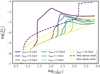 |
Fig. 2 Total energy in CRs in units of 1051 erg for the LBV (solid) and RSG cases (dashed) as a function of time. |
3.2 Gamma-ray emission and detectability
We calculated the gamma-ray emission as described in Appendix A.1 and applied the γγabsorption as described in Appendix A.6. First, we discuss the emission in the 1–10 TeV (hereafter VHE) and 1–300 GeV (hereafter Fermi) energy bands. Additionally, we evaluated the gamma-ray detectability in the energy ranges for various current and future instruments, which are only shown in visibility plots in Section 3.2.2 and in Appendix B.
3.2.1 Gamma-ray emission
We derived the γ-ray luminosity in the VHE and Fermi bands by only accounting for hadronic emission. We considered a standard ISM composition for the CSM material, even though a heavier composition can be expected in the vicinity of massive stars. A heavier composition would not affect the light curves or luminosity considerably, but might change the spectrum shape of the gamma-ray emission, especially at energies below 1 GeV (Bhatt et al. 2020; de Oña Wilhelmi et al. 2020).
Figure 3 illustrates the evolution of the γ-ray luminosity for our LBV and RSG models. The shock-shell interactions are clearly visible as peaks in the γ-ray emission after the initial peak around tens of days that is caused by the interaction with the smooth wind. The peaks caused by the interactions exceed the initial peak luminosities for LBV scenarios with interactions in the first two years, and for the RSG scenario with the massive shell. It is noteworthy that most IACTs undertake their pointed observations in the first weeks after the explosion and might thus miss late interactions.
The γ-ray emission can in the most extreme case of a LBV progenitor and an interaction after ≈36 days be five (three) orders of magnitude more luminous in the VHE (Fermi) band compared to the early-time emission. This underlines that shock-shell interactions strongly enhance the detection prospects of γ-ray emission from these objects. The interaction of the shock in the massive RSG-shell scenario still exceeds the initial luminosity by about one order of magnitude in the Fermi band and by two orders of magnitude in the VHE band because the γγabsorption is stronger at higher energies.
Gamma-ray luminosities as high as 1043 erg s−1 were reached in the VHE and Fermi-LAT bands for an early-interacting Type IIn SNR and 1040 and 1041 erg s−1 for a Type IIP SNR interacting with a dense shell in the VHE and Fermi bands, respectively. These predictions are well above the current upper limits of the High-Energy Stereoscopic System (H.E.S.S.) of ≤1.5 · 1039 erg s−1 for nearby Type IIP events (H.E.S.S. Collaboration 2019). These observations were performed within the first year after explosion, however, where the flux in the VHE band does not exceed 2 × 1038 erg s−1 because the γγabsorption is strong and the densities are very low. A close-by Type IIn explosion might have been detectable, but no event occurred close enough to trigger H.E.S.S. observations.
Interestingly, our heavy Type IIP scenario produces a gamma-ray luminosity that is high enough to explain the detection of SN 2004dj in Fermi-LAT data about 5 years after the explosion (Xi et al. 2020). Unfortunately, the SN occurred before the launch of Fermi-LAT, but the onset of the observations coincided with the expected time for the shock-shell interaction in our models, as does the ≈5 year interval over which the signal faded. Xi et al. (2020) reported a luminosity of ≈1039 erg s−1, which is in in the middle of our predicted luminosity range: 3 × 1037−1041 erg s−1. Recently, Martí-Devesa et al. (2024) observed the Type IIP SNe SN 2023ixf located 6.85 Mpc from Earth and established a luminosity limit of Lγ(E > 1 GeV) ≤ 6 · 1040−3.4 · 1041 erg. This limit is consistent with our prediction for the early-time emission in the freely expanding wind. After the shell interaction, our predicted peak luminosity for the dense-shell case reaches the detection limit, if such a dense shell were present in the CSM of SN 2023ixf.
Our reference model from Paper I used an unrealistically high mass-loss rate of 10−2 M⊙ yr−1. The peak luminosity of our shell-interaction model still surpasses the luminosity of our previous LBV model by a factor of ≈5 in the VHE band and reaches the same luminosity in the Fermi band, which is less affected by γγabsorption.
The different absorption processes involved and the dynamic evolution of the particle spectrum during the interaction create considerable time shifts between the emission peaks in different energy bands. In the earliest Type IIn interaction, the first peak in the HE gamma-ray emission occurs at ≈85 days, followed by a peak in the VHE domain after ≈100 days, and followed by a peak after about 150 days for the radio emission (see Section 3.3). This poses an exceptional observational challenge in detecting these events as the HE observatories operate in a survey mode and might only acquire enough photons after the VHE emission has peaked. Usually, the gamma-ray emission fades already when the source peaks in the radio. The time delay between HE and VHE gamma-ray emission can be longer for later interactions because the acceleration time for the highest-energy particles becomes longer.
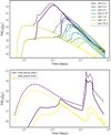 |
Fig. 3 Gamma-ray luminosities in the Fermi-LAT energy range (dashed) and H.E.S.S. energy range (solid) accounting for γγ absorption. Top: SNR of LBV progenitors interacting with the dense shell at different times (models as described in Table 1). The γγ absorption has ceased completely after about 200 days. Bottom: interaction of SNRs with RSG progenitors interacting with dense shells created by external photoionization. The purple case represents an upper limit in terms of shell mass, cause by a high mass-loss wind and a strong ambient photon field. The diluted case represents typical parameters for the population of RSGs (see Table 1 for details). |
3.2.2 Gamma-ray detectability
We evaluated the detectability of the emission for various current and future gamma-ray observatories. For compactness, the corresponding plots are presented in Appendix B.
We used the sensitivity from the Fermi-LAT collaboration3 and from Vernetto & LHAASO Collaboration (2016) and Cherenkov Telescope Array Observatory and Cherenkov Telescope Array Consortium (2021) to estimate the detection horizon for the survey instruments Fermi-LAT, HAWC, LHAASO, and the IACTs H.E.S.S4. and CTAO-South. We also included the projected eASTROGAM sensitivity from De Angelis et al. (2017). For the IACTs, we compared the flux at any given time during the remnant evolution with the detection sensitivity for 50h of observations. For the survey-like instruments, the required observation times can be longer than the duration of our transient signal. Therefore, we integrated the photon flux since the explosion of the SN, denoted here as t, and compared the accumulated flux to the detectio -sensitivity of the instruments scaled by  , where tref denotes the observation time indicated for the sensitivity curves of Fermi-LAT, HAWC, and instruments like them.
Fermi-LAT is the most sensitive gamma-ray telescope operating in the HE gamma-ray domain in survey mode, thus observing the whole sky continuously. It is therefore expected to play an extraordinary role in detecting gamma-ray emission from nearby SNe and their remnants. Figure 4 shows the Fermi-LAT detectability of our two RSG scenarios and the LBV scenarios for interactions at 36 days and 2 years, respectively. An early-interacting SNR would be detectable out to roughly 80 Mpc, although the significance rises only with the onset of the shell interaction after 36 days. The late interaction (after 2 years) would have a considerably smaller detection horizon of only 5 Mpc, and the rise in significance would again only occur with the onset of the interaction. The RSG scenario with the heavy shell enables a detection of up to 6 Mpc, while the low-mass shell interaction is only visible for SNe occurring within 600 kpc5.
Since 2015, the Transient Name Server6 lists a total of 39 firmly identified Type IIn explosions that occurred at distances closer than 75 Mpc and one explosion (SN 2019el) at a distance closer than 6 Mpc. In the same time frame, only one Type IIP event occurred at a distance closer than 10 Mpc (SN 2016cok), that is, at the edge of detectability if a shell interaction occurs.
The recent nearby and bright type II SN 2023ixf and SN 2024ggi lack a clear classification into either of these explosion types, although they are arguably the best candidates for gamma-ray detection on account of their proximity and evidence of circumstellar interaction.
The prospects at MeV energies using the proposed eAS-TROGAM (De Angelis et al. 2017), for instance, are similar, but limited to about half the distances of Fermi-LAT due to the pion-bump feature at lower energies (see also Figure B.1).
Similarly to the increased detectability with Fermi-LAT, when shock-shell interactions take place, the detection prospects also increase in the VHE domain using H.E.S.S. and other current-generation IACTs. Fig. B.2 shows the VHE detectability of the same simulations as Fig. 4 using the sensitivity curve for H.E.S.S. as representative for the current generation of IACTs. The detection horizon increases to ≈190(1.75) Mpc for an early-(late-) interacting Type IIn explosion and ≈10(0.6) Mpc for the massive (low-mass) RSG shell. The detection prospects are best after ≈100 days and 5 years for the LBV and RSG scenario, respectively. The peak detectability and onset of the interaction shift by about 100–1200 days in the LBV cases because the particles need time to become accelerated to energies at which they radiate in the VHE domain. The peak in the HE domain is reached earlier, between 75 and 270 days after the onset of the interaction. An overview of the peak times in the different wavebands is shown in Table 2 and is further discussed in Section 4.
The Transient Name Server lists a total of 94 SNe since 2015 that were close enough to be detected by H.E.S.S. in case of an early interaction, but none for a late interaction.
Observational indications of late-time interactions with CSM shells are rare so far, and more late-time observations are needed for a reliable estimate of the number of potentially detectable SNe. The recent study by Soria et al. (2025) found evidence for a brightening by at least two orders of magnitude in the radio band of the Type IIb SNe SN 2001ig roughly 20 years after the explosion.
Of the type IIP SNe since 2015, only SN 2016cok might be close enough for the detection of the RSG-shell interaction. The large potential number of SNe that might be detectable with H.E.S.S. illustrates the need for a carefully crafted observation strategy. Without a trigger criterion for the onset of shock-shell interactions, no monitoring of all potential SNRs is possible.
H.E.S.S. Collaboration (2019) observed SN 2008bk, for instance, which was a Type IIP explosion at a distance of 4 ± 0.4 Mpc. It might have been visible to H.E.S.S. if it had interacted with a circumstellar shell. Because of the distance and because the H.E.S.S. observations took place within the first year of explosion, however, the explosion would have needed to take place at least four times closer to Earth in order to be detectable.
HAWC and LHAASO both operate in survey mode, but at slightly different energy ranges. In principle, SNe should be detectable to 60(0.5) Mpc and 4(0.175) Mpc for HAWC and 70(0.15) Mpc and 6(0.2) Mpc for LHAASO for the early (late) LBV and heavy (light) RSG scenarios, respectively, as shown in Figs. B.3 and B.5, respectively. This is again considerably farther than for the smooth-wind case (Paper I). In the case of LHAASO, the detectability horizon not only reflects the change in luminosity due to the different shell density, but also the fact that later interactions lack the boost to Emax and thus have a cutoff in the energy range in which LHAASO is most sensitive. For both experiments, a total of 19 and 28 Type IIn SNe were close enough to potentially be detected for early interactions, while SN2016cok remains the only Type IIP explosion that occurred close enough for a potential detection. No explosion occurred close enough to be detectable for a late interaction or a light RSG shell.
CTAO-South is the only telescope that is still under construction and is considered here. The detectability distributions for CTAO-South appear to be similar to those of H.E.S.S., but extend to much larger distances. By reaching 300(3) Mpc for the Type IIn case, CTAO-South will probe distances at which EBL absorption becomes a factor. Type IIP explosions still only remain detectable in the vicinity up to ≈20(1.2) Mpc. While CTAO-South might have been able to follow-up on 94 Type IIn explosions, similar to the existing IACTs, there are 6 additional Type IIP events that are below the optimistic detection threshold.
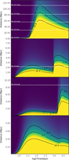 |
Fig. 4 Fermi detectability for LBV 0.1, LBV 2.0, and RSG high-mass and RSG low-mass scenarios, from top to bottom. The white lines indicate detected SNe explosions at their inferred distance and their overlap with the operation window of Fermi-LAT. Type IIn events are shown in the upper two panels, and Type IIP events are shown in the lower panels. |
Time of first interaction with the shell and time until the peak in the corresponding waveband after the onset of the interaction.
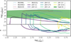 |
Fig. 5 Top panel: radio luminosity, including the effects of free-free absorption for Type IIn explosions. The green area indicates the 1σ uncertainty region for the rise time and peak radio luminosity for Type IIn SN taken from Bietenholz et al. (2021). Bottom panel: radio spectral index α of the absorbed radio flux at 4 GHz. |
3.3 Radio emission
We calculated the radio emission based on the electron distribution and the magnetic field, including the self-amplified component using the method described by Paper I. Figures 5 and 6 show the radio luminosity at 4 GHz, including the effects of free-free absorption in the CSM and the evolution of the radio spectral index for the LBV and RSG shell-interaction simulations, respectively. Where Paper I struggled to explain the observed peak luminosity of the radio emission either by strong free-free absorption or by too low magnetic fields for moderate mass loss, the shock-shell interaction overcomes the two shortcomings in the LBV scenarios. As soon as the shock has passed the majority of the dense shell, the radio emission can freely escape, whereas the interaction itself boosts the magnetic field amplification to levels that are commensurate with the observed radio-flux. The observed peak now agrees well with the population study of radio SNe from Bietenholz et al. (2021). We also added the observed radio light curves for a number of SNe in both plots. While the onset of our predicted emission roughly agrees with the measurements, our predicted luminosities appear to be slightly too low, but the best-charcterized SNe in this sample from Bietenholz et al. (2021) also tend to be the brightest SNe. We also added the light curve for SN 2001ig, where a sign of radio-rebrightening was recently detected (Soria et al. 2025). In addition to the classification of SN 2001ig as a Type IIb event, the observed luminosity of the rebrightening matches our prediction for a shell interaction well.
Interestingly, the shell interaction affects the radio spectral index by softening it. When absorption becomes negligible, the radio index is softer than α = −0.5, and it reaches values as low as α = −0.75 in the Type IIn scenarios, but hardens gradually over time because during the shell interaction at each successive time, more particles are injected than before. As the acceleration is not instantaneous, this softens the spectrum. The effect fades when the shock has passed the shell, and when recently accelerated particles start to dominate, the spectrum hardens. A similar effect of a gradual hardening of the ratio, starting from a soft spectrum, is observed for SN1987A (Zanardo et al. 2010). There, the shock interacted with a dense equatorial ring that sparked a strong brightening in the radio and X-ray emission of the remnant. This situation is comparable to our simulation setup despite the different geometry.
The Type IIP scenarios show a double-peak structure in which a first peak emerges after several hundred days in the low-mass case, followed by a second peak at the shock-shell interaction. The spectrum is dominated by a nonthermal spectrum when the shock passed most of the shell, and the spectral index reached α ≈ −0.5 rather quickly. In the high-mass case, the first peak is suppressed because the absorption in the denser shell is stronger. The shock-shell interaction boosts the radio emission, but the spectrum appears to be thermal as the high shell mass compared to the ejecta mass slows the shock down considerably and prevents the formation of a nonthermal spectrum in this case. The nonthermal radio emission starts to rise ≈15 years after the explosion only after the shock is reaccelerated.
Observations suggest radio spectra that are even softer than α ≈ −0.75 for Type Ib and Type Ic SN, indicating electron-spectra as soft as s = −3 (Chevalier & Fransson 2006). Type IIP explosions, on the other hand, were modeled with electron spectra closer to s = −2.2. Chevalier et al. (2006) pointed out that cooling can significantly soften the spectra in these cases.
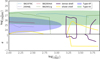 |
Fig. 6 Same as Figure 5, but for the RSG and Type IIP scenarios. The average of the Type IIP population is taken from Bietenholz et al. (2021). |
3.4 Thermal X-ray emission
As a proxy for the thermal X-ray emission, we followed the ansatz described in Appendices A.2 and A.5. In both progenitor cases, the interaction with the shell strongly boosts the thermal X-ray emission by up to five orders of magnitude for the LBVs and by four orders of magnitude for the RSGs. The boost in the LBV case has to be considered as an upper limit, however, because the shock is radiative for the high densities during the shell interaction.
Figure 7 shows that our predicted X-ray emission is roughly consistent with the observational constraints. X-rays from LBVs are not detected experimentally before approximately one year after the explosion, however, which might simply be an observational bias or might indicate typically larger distances of the shells from the SN progenitor.
For Type IIP explosions, our early emission basically agrees with the observations by design because we used typical mass-loss rates. The shell interaction then greatly enhances this emission. At the onset of the interaction after a few years, however, targeted X-ray observations of previously detected SNe are rare because no coordinated long-term monitoring program exists. These rebrightening events are therefore very probably missed observationally. Only an X-ray survey instrument can realistically hope to detect these shell-interaction events without a trigger from another waveband.
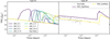 |
Fig. 7 Absorbed thermal X-ray luminosity between 0.2 and 10 keV for Type IIn explosions (left) and Type IIP explosions (right). The gray stars indicate the measurements listed by Dwarkadas (2014). |
3.5 Optical emission
The difficulty of detecting shock-shell interactions, especially for RSG progenitors, is the long time-offset between the interaction and the explosion. Here, targeted observations as carried out in the radio or X-ray band are rare this late after the explosions, and many potentially interesting interactions might therefore be missed. A search for flaring transients with Fermi-LAT might be a way at present to provide triggers, but a sufficiently large observation window is required. Further, future IACTs have a notably farther detection horizon, so that Fermi-LAT would not be sensitive enough to provide triggers for CTAO, for example.
An alternative are the currently operating high-cadence optical surveys such as the ZTF (Bellm et al. 2019), Pan-STARRS (Hodapp et al. 2004), or Gaia (Hodgkin et al. 2013), which regularly monitor large parts of the night sky. Following the ansatz described in Appendix A.3, we calculated the optical emission expected from the interaction for the RSG cases. Figure 8 shows the optical luminosity in the B band and the ratio of the B- and R-band luminosities for the RSG case. The shell interaction gives rise to enhanced X-ray emission and likewise to optical emission that is (depending on the shell mass) lower by 5 orders of magnitude than the peak of the emission from the SN photosphere. This means that the most dense SNR-shell interactions for RSGs might be detectable out to a few megaparsec, given the detection horizon of Type IIP SNe of up to a few hundred megaparsec. Less dense shells are considerably weaker in their optical emission, however, and are hence harder to detect.
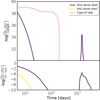 |
Fig. 8 Top: optical light curves in the B band (398–492 nm) for an SN interaction with the two RSG shells (solid lines) and the luminosity from the SN photosphere (dotted red line). Bottom: ratio of the B- and R-band (591–727 nm) luminosities over time. |
4 Observation strategy
Our work suggests that current observation strategies for detecting gamma-ray emission from CC-SNe can be improved. The initial γγabsorption attenuates the signal, while the rise in the light curves associated with the potential shock-shell interaction can occur rather late (Milisavljevic et al. 2015). A fundamental problem in detecting the gamma-ray emission from CC-SNe in our scenarios therefore is the definition of a suitable trigger for targeted observations.
Table 2 indicates that the X-ray emission peaks first in practically all cases, as it directly reflects the change in the ISM density. Fermi-LAT, where the peak luminosity is reached tens of days after the peak on thermal X-rays, therefore is the only survey instrument in the HE domain that is currently operational. Depending on the source flux, it requires integration times of tens to hundreds of days for a detection. The emission at VHE energies peaks in general after the peak in HE energies is reached. As a consequence, the emission peak as detectable with IACTs might therefore be missed because Fermi-LAT needs a considerable amount of integration time to detect a signal. The radio emission in general peaks last due to the absorption in the dense shell. On the other hand, radio observations have the potential to monitor nearby SNe for signals of rebrightening, as was done for SN 2001ig (Soria et al. 2025). We note, however, that the timing in Table 2 is idealized in our spherically symmetric treatment and might be altered, especially smeared, if the explosions itself or the CSM structure differs significantly from spherical symmetry.
Emission in the optical might also provide good prospects for a detection because large parts of the sky can be monitored with a high cadence. For a potential detection in radio, a timely communication to the high-energy community is crucial for a chance of a detection in gamma-rays.
Furthermore, our Type IIn models clearly show that the peak in the gamma-ray emission coincides more closely with the peak in the radio emission than with the optical emission of the SN explosion. The shell interaction increases the target density for pion production, and the higher ambient density means that more particles (including electrons) can be accelerated. A brightening in radio and gamma-rays therefore has a common origin. Again, the position of the (first) peak in the radio emission can be hundreds to thousands of days after the explosion. This is considerably later than the current timescales for follow-up observations.
Possible follow-up instruments in the centimeter and millimeter radio bands are MeerKAT (Jonas & MeerKAT Team 2016) and the Atacama Large Millimeter Array (ALMA, Wootten & Thompson 2009). They are currently the most sensitive instruments in their wavelength regime. For sensitivities of 50 µJy bm−1 at 100 GHz, and 15 µJy bm−1 at 3 GHz (for a 15 minute ALMA integration and a 12 minute MeerKAT integration, respectively), our models predict that the emission is always first detectable in the ALMA band. For the cases we considered, the shortest timescale at which the source would be detectable for LBVs occurs for the LBV 10.0 case (as early as one week after the explosion for a distance of 1 Mpc), and the longest timescale holds for LBV 2.0 (where emission is not detectable until two years after the explosion, also for a distance of 1 Mpc). For the RSG cases, the emission is expected to be detectable with ALMA in the first five days after the explosion (for the low-mass case) and in the first three weeks (for the high-mass case), again for a distance of 1 Mpc. The time for a detection of the emission with MeerKAT after an ALMA detection varies on a timescale of days to years for the cases we considered.
For this reason, radio observations can provide important diagnostics that might be used as triggers for deep gamma-ray observations. In several cases, the ALMA detections occur well ahead of the shell interaction, and they can track the brightening associated with it. The lower radio frequency observations probe the absorption or lack thereof due to the presence of a shells of different masses and distances to the star. When combined, it is possible to distinguish between the cases and to constrain the scenario represented by a given event, and hence, the best time for conducting the costly gamma-ray observations. This strategy of monitoring the radio luminosity with ALMA or MeerKAT is likely feasible for the few SNe that occur within ≲25 Mpc.
In addition to a dedicated ALMA target-of-opportunity project as suggested above, the gamma-ray community would benefit from closer and more timely communication with the many teams that follow nearby SNe with a wide variety of radio facilities, such as the Karl G. Jansky Very Large Array (JVLA), the Giant Metre Wave Radio Telescope (GMRT), or the Australia Telescope Compact Array (ATCA), often for years after the explosion.
It is worth noting that the cases we discussed here are physically distinct from observed SN such as SN 2024ggi, where a dense CSM was detected up to roughly 2.3 × 10⁻¹⁴cm around the progenitor with a mass-loss rate of roughly Ṁ = 10−2M⊙ yr−1 and vwind = 40 km s−1 (Shrestha et al. 2024). Similarly, a dense CSM extending to r ≈ 1015 cm was inferred from modeling SN 2023ixf (e.g. Kozyreva et al. 2025). These values roughly correspond to the density setup for the free wind in our LBV scenarios. Our models clearly show, however, that an event like this would only be detectable to distances of up to 4 Mpc depending on the instrument, while SN 2024ggi occurred at a distance of roughly 7 Mpc. Further, the small extension of the dense CSM in this case means that a high internal gamma-ray luminosity is only achieved within the first few days after the explosion, where γγabsorption is strong and efficiently attenuates the signal (see also Paper I). Cases such as SN 2024ggi are likely linked to enhanced RSG mass loss just prior to their explosion (Bruch et al. 2021), but do not create the additional shell-like structures we discussed here.
5 Conclusions
We performed numerical simulations of particle acceleration in very young SNRs that expand in dense circumstellar media and feature dense shells created by the progenitors by solving time-dependent transport equations of CRs and magnetic turbulence in the test-particle limit alongside the standard gas-dynamical equations for CC SNRs.
The peak luminosity in the γ-ray domain that is reached during the shock-shell interaction clearly exceeds the initial luminosities of the first weeks after the explosion (which are strongly affected by γγabsorption). In the VHE domain, the peak luminosity during the interaction is higher by about a factor of 5 than the luminosity expected from a progenitor with a smooth wind, which is is denser by about a factor of 100 than the case that we considered. We obtained luminosties of up to 1043 erg s−1 for early-interacting Type IIn explosions and 1040 and 1041 erg s−1 for the light and heavy shell models of RSG progenitors.
We investigated the radio emission and took the effect of free-free absorption in the ambient medium into account. We found peak luminosities that were consistent with the population average for Type IIn explosions. The radio spectral index appeared to be softer than α = −0.5 immediately after the free-free absorption became negligible and the emission detectable, and it gradually hardened toward the canonical α = −0.5, similar to the evolution observed for SN 1987A.
The late peak of the gamma-ray emission differs from current observation strategies of IACTs. After evaluating the thermal emission in the optical and x-rays, which both peak after the gamma-ray emission, we identified high-cadence optical surveys as a potentially suitable tool for capturing the most extreme Type IIPs that interact with dense shells. The small sample sizes in the nearby Universe and the short required observation times mean that a systematic radio and mm monitoring of close-by SNe for a few years after their explosions might prove valuable for identifying late shell-interactions as well.
Current-generation instruments can detect LBV-shell interaction up to 80 and 190 Mpc for the most extreme cases, while RSG-shell interactions are only visible up to 6 and 10 Mpc for Fermi-LAT and H.E.S.S., respectively. CTAO might push these boundaries to 300 and 20 Mpc for our most extreme LBV and RSG scenarios.
Acknowledgements
R.B. and J.M. acknowledge funding from an Irish Research Council Starting Laureate Award. J.M. acknowledges funding from a Royal Society-Science Foundation Ireland University Research Fellowship. This publication results from research conducted with the financial support of Taighde Éireann - Research Ireland under Grant numbers 20/RS-URF-R/3712, IRCLA\2017\83. We acknowledge the SFI/HEA Irish Centre for High-End Computing (ICHEC) for the provision of computational facilities and support (project dsast026c). I.S. acknowledges funding from Comunidad de Madrid through the Atracción de Talento “César Nombela” grant with reference number 2023-T1/TEC-29126. We are grateful to Morgan Fraser and Takashi Moriya for their valuable input and discussions on the paper.
References
- Abdalla, H., Aharonian, F., Ait-Benkhali, F., et al. 2021, Proc. Int. Cosmic Ray Conf., 395, 809 [Google Scholar]
- Abeysekara, A. U., Archer, A., Benbow, W., et al. 2020, ApJ, 894, 51 [NASA ADS] [CrossRef] [Google Scholar]
- Acciari, V. A., Ansoldi, S., Antonelli, L. A., et al. 2022, Nat. Astron., 6, 689 [NASA ADS] [CrossRef] [Google Scholar]
- Ackermann, M., Ajello, M., Albert, A., et al. 2014, Science, 345, 554 [NASA ADS] [CrossRef] [Google Scholar]
- Ackermann, M., Arcavi, I., Baldini, L., et al. 2015, ApJ, 807, 169 [CrossRef] [Google Scholar]
- Astropy Collaboration (Price-Whelan, A. M., et al.) 2018, AJ, 156, 123 [Google Scholar]
- Baade, W., & Zwicky, F. 1934, Proc. Natl. Acad. Sci., 20, 259 [NASA ADS] [CrossRef] [Google Scholar]
- Bell, A. R., Schure, K. M., Reville, B., & Giacinti, G. 2013, MNRAS, 431, 415 [Google Scholar]
- Bellm, E. C., Kulkarni, S. R., Graham, M. J., et al. 2019, PASP, 131, 018002 [Google Scholar]
- Bhatt, M., Sushch, I., Pohl, M., et al. 2020, Astropart. Phys., 123, 102490 [NASA ADS] [CrossRef] [Google Scholar]
- Bietenholz, M. F., Bartel, N., Argo, M., et al. 2021, ApJ, 908, 75 [NASA ADS] [CrossRef] [Google Scholar]
- Blandford, R., & Eichler, D. 1987, Phys. Rep., 154, 1 [Google Scholar]
- Brose, R., Telezhinsky, I., & Pohl, M. 2016, A&A, 593, A20 [NASA ADS] [CrossRef] [EDP Sciences] [Google Scholar]
- Brose, R., Pohl, M., & Sushch, I. 2021, A&A, 654, A139 [NASA ADS] [CrossRef] [EDP Sciences] [Google Scholar]
- Brose, R., Sushch, I., & Mackey, J. 2022, MNRAS, 516, 492 [NASA ADS] [CrossRef] [Google Scholar]
- Brose, R., Sushch, I., & Mackey, J. 2025, A&A, 699, A160 [NASA ADS] [CrossRef] [EDP Sciences] [Google Scholar]
- Bruch, R. J., Gal-Yam, A., Schulze, S., et al. 2021, ApJ, 912, 46 [NASA ADS] [CrossRef] [Google Scholar]
- Cherenkov Telescope Array Observatory and Cherenkov Telescope Array Consortium. 2021, CTAO Instrument Response Functions - prod5 version v0.1 [Google Scholar]
- Chevalier, R. A., & Fransson, C. 2006, ApJ, 651, 381 [NASA ADS] [CrossRef] [Google Scholar]
- Chevalier, R. A., Fransson, C., & Nymark, T. K. 2006, ApJ, 641, 1029 [NASA ADS] [CrossRef] [Google Scholar]
- Cold, C., & Hjorth, J. 2023, A&A, 670, A48 [NASA ADS] [CrossRef] [EDP Sciences] [Google Scholar]
- Cristofari, P., Blasi, P., & Amato, E. 2020a, Astropart. Phys., 123, 102492 [Google Scholar]
- Cristofari, P., Renaud, M., Marcowith, A., Dwarkadas, V. V., & Tatischeff, V. 2020b, MNRAS, 494, 2760 [NASA ADS] [CrossRef] [Google Scholar]
- Cristofari, P., Marcowith, A., Renaud, M., et al. 2022, MNRAS, 511, 3321 [Google Scholar]
- Dastidar, R., Misra, K., Hosseinzadeh, G., et al. 2018, MNRAS, 479, 2421 [NASA ADS] [CrossRef] [Google Scholar]
- De Angelis, A., Tatischeff, V., Tavani, M., et al. 2017, Exp. Astron., 44, 25 [NASA ADS] [CrossRef] [Google Scholar]
- de Oña Wilhelmi, E., Sushch, I., Brose, R., et al. 2020, MNRAS, 497, 3581 [CrossRef] [Google Scholar]
- Diesing, R. 2023, ApJ, 958, 3 [NASA ADS] [CrossRef] [Google Scholar]
- Dubus, G. 2006, A&A, 451, 9 [NASA ADS] [CrossRef] [EDP Sciences] [Google Scholar]
- Dwarkadas, V. V. 2014, MNRAS, 440, 1917 [Google Scholar]
- Dwarkadas, V. V. 2025, Universe, 11, 161 [Google Scholar]
- Finke, J. D., Razzaque, S., & Dermer, C. D. 2010, ApJ, 712, 238 [NASA ADS] [CrossRef] [Google Scholar]
- Fox, O. D., Filippenko, A. V., Skrutskie, M. F., et al. 2013, AJ, 146, 2 [NASA ADS] [CrossRef] [Google Scholar]
- Gal-Yam, A. 2021, AAS Meeting Abs., 237, 423.05 [Google Scholar]
- Gould, R. J., & Schréder, G. 1966, Phys. Rev. Lett., 16, 252 [NASA ADS] [CrossRef] [Google Scholar]
- Gould, R. J., & Schréder, G. P. 1967, Phys. Rev., 155, 1404 [Google Scholar]
- Grassitelli, L., Langer, N., Mackey, J., et al. 2021, A&A, 647, A99 [NASA ADS] [CrossRef] [EDP Sciences] [Google Scholar]
- H.E.S.S. Collaboration (Abdalla, H., et al.) 2019, A&A, 626, A57 [NASA ADS] [CrossRef] [EDP Sciences] [Google Scholar]
- H.E.S.S. Collaboration (Aharonian, F., et al.) 2022, Science, 376, 77 [NASA ADS] [CrossRef] [Google Scholar]
- Hnatyk, B., & Petruk, O. 1999, A&A, 344, 295 [NASA ADS] [Google Scholar]
- Hodapp, K. W., Kaiser, N., Aussel, H., et al. 2004, Astron. Nachr., 325, 636 [Google Scholar]
- Hodgkin, S. T., Wyrzykowski, L., Blagorodnova, N., & Koposov, S. 2013, Phil. Trans. Royal Soc. London Ser. A, 371, 20120239 [Google Scholar]
- Huang, C. Y., Park, S. E., Pohl, M., & Daniels, C. D. 2007, Astropart. Phys., 27, 429 [Google Scholar]
- Inoue, T., Marcowith, A., Giacinti, G., Jan van Marle, A., & Nishino, S. 2021, ApJ, 922, 7 [NASA ADS] [CrossRef] [Google Scholar]
- Jacobson-Galán, W. V., Dessart, L., Jones, D. O., et al. 2022, ApJ, 924, 15 [CrossRef] [Google Scholar]
- Jacobson-Galán, W. V., Dessart, L., Davis, K. W., et al. 2025, ApJ, 992, 100 [Google Scholar]
- Jauch, J. M., & Rohrlich, F. 1976, The Theory of Photons and Electrons. The Relativistic Quantum Field Theory of Charged Particles with Spin One-half (Berlin: Springer) [Google Scholar]
- Jonas, J., & MeerKAT Team 2016, in MeerKAT Science: On the Pathway to the SKA, 1 [Google Scholar]
- Kozyreva, A., Caputo, A., Baklanov, P., Mironov, A., & Janka, H.-T. 2025, A&A, 694, A319 [NASA ADS] [CrossRef] [EDP Sciences] [Google Scholar]
- Langer, N. 2012, ARA&A, 50, 107 [Google Scholar]
- Lundqvist, P., & Fransson, C. 1996, ApJ, 464, 924 [NASA ADS] [CrossRef] [Google Scholar]
- Mackey, J., Mohamed, S., Gvaramadze, V. V., et al. 2014, Nature, 512, 282 [Google Scholar]
- Mackey, J., Castro, N., Fossati, L., & Langer, N. 2015, A&A, 582, A24 [NASA ADS] [CrossRef] [EDP Sciences] [Google Scholar]
- Mackey, J., Walch, S., Seifried, D., et al. 2019, MNRAS, 486, 1094 [Google Scholar]
- Mackey, J., Green, S., Moutzouri, M., et al. 2021, MNRAS, 504, 983 [NASA ADS] [CrossRef] [Google Scholar]
- Marcowith, A., Dwarkadas, V. V., Renaud, M., Tatischeff, V., & Giacinti, G. 2018, MNRAS, 479, 4470 [CrossRef] [Google Scholar]
- Marti-Devesa, G., & Fermi-LAT Collaboration 2024, ATel, 16601, 1 [Google Scholar]
- Martí-Devesa, G., Cheung, C. C., Di Lalla, N., et al. 2024, A&A, 686, A254 [NASA ADS] [CrossRef] [EDP Sciences] [Google Scholar]
- Matsuoka, T., Maeda, K., Kimura, S. S., & Tanaka, M. 2025, arXiv e-prints [arXiv:2505.06609] [Google Scholar]
- Mezger, P. G., & Henderson, A. P. 1967, ApJ, 147, 471 [Google Scholar]
- Mignone, A., Bodo, G., Massaglia, S., et al. 2007, ApJS, 170, 228 [Google Scholar]
- Milisavljevic, D., Margutti, R., Kamble, A., et al. 2015, ApJ, 815, 120 [NASA ADS] [CrossRef] [Google Scholar]
- Moran, S., Fraser, M., Kotak, R., et al. 2023, A&A, 669, A51 [NASA ADS] [CrossRef] [EDP Sciences] [Google Scholar]
- Moriya, T. J., Blinnikov, S. I., Tominaga, N., et al. 2013, MNRAS, 428, 1020 [NASA ADS] [CrossRef] [Google Scholar]
- Morrison, R., & McCammon, D. 1983, ApJ, 270, 119 [Google Scholar]
- Murase, K., Thompson, T. A., Lacki, B. C., & Beacom, J. F. 2011, Phys. Rev. D, 84, 043003 [NASA ADS] [CrossRef] [Google Scholar]
- Murase, K., Thompson, T. A., & Ofek, E. O. 2014, MNRAS, 440, 2528 [Google Scholar]
- Prokhorov, D. A., Moraghan, A., & Vink, J. 2021, MNRAS, 505, 1413 [NASA ADS] [CrossRef] [Google Scholar]
- Shrestha, M., Bostroem, K. A., Sand, D. J., et al. 2024, ApJ, 972, L15 [Google Scholar]
- Shvartzvald, Y., Waxman, E., Gal-Yam, A., et al. 2024, ApJ, 964, 74 [NASA ADS] [CrossRef] [Google Scholar]
- Skilling, J. 1975, MNRAS, 172, 557 [CrossRef] [Google Scholar]
- Smith, N. 2014, ARA&A, 52, 487 [Google Scholar]
- Smith, N., Hinkle, K. H., & Ryde, N. 2009, AJ, 137, 3558 [NASA ADS] [CrossRef] [Google Scholar]
- Smith, N., Li, W., Filippenko, A. V., & Chornock, R. 2011, MNRAS, 412, 1522 [NASA ADS] [CrossRef] [Google Scholar]
- Soria, R., Russell, T. D., Wiston, E., et al. 2025, PASA, 42, e050 [Google Scholar]
- Sturner, S. J., Skibo, J. G., Dermer, C. D., & Mattox, J. R. 1997, ApJ, 490, 619 [NASA ADS] [CrossRef] [Google Scholar]
- Sushch, I., & van Soelen, B. 2017, ApJ, 837, 175 [NASA ADS] [CrossRef] [Google Scholar]
- Sushch, I., Blasi, P., & Brose, R. 2025, A&A, 700, A37 [NASA ADS] [CrossRef] [EDP Sciences] [Google Scholar]
- Taddia, F., Stritzinger, M. D., Fransson, C., et al. 2020, A&A, 638, A92 [NASA ADS] [CrossRef] [EDP Sciences] [Google Scholar]
- Tatischeff, V. 2009, A&A, 499, 191 [NASA ADS] [CrossRef] [EDP Sciences] [Google Scholar]
- Telezhinsky, I., Dwarkadas, V., & Pohl, M. 2013, AAS/High Energy Astrophys. Div., 13, 127.16 [Google Scholar]
- Vernetto, S., & LHAASO Collaboration 2016, J. Phys. Conf. Ser., 718, 052043 [NASA ADS] [CrossRef] [Google Scholar]
- Wootten, A., & Thompson, A. R. 2009, IEEE Proc., 97, 1463 [NASA ADS] [CrossRef] [Google Scholar]
- Xi, S.-Q., Liu, R.-Y., Wang, X.-Y., et al. 2020, ApJ, 896, L33 [NASA ADS] [CrossRef] [Google Scholar]
- Yuan, Q., Liao, N.-H., Xin, Y.-L., et al. 2018, ApJ, 854, L18 [NASA ADS] [CrossRef] [Google Scholar]
- Zanardo, G., Staveley-Smith, L., Ball, L., et al. 2010, ApJ, 710, 1515 [Google Scholar]
The estimated distance is 6.85 Mpc.
The external photon field around RSGs (see also Section 2.1.2) might provide additional seed-photons but is orders of magnitude below the energy density of photons from the SN-photosphere and might only get relevant at significantly later times than the ones considered here.
Here taken as a representative of all current-generation IACTs.
These numbers are somewhat higher than the values in Paper I where, due to a bug in the production of the detectability plots, the denotes distances are too small by a factor of ≈25. An erratum is in preparation.
The transient name server (Gal-Yam 2021, https://www.wis-tns.org/) is the official channel to assign and classify transients by the IAU since 2015.
This corresponds to the wavelengths of the upcoming ULTRASAT mission Shvartzvald et al. 2024.
Appendix A Radiation and absorption processes
A.1 Nonthermal emission
The nonthermal emission of the accelerated particles is calculated in a spatially dependent manner, taking into account the local particle distribution and magnetic field strength in case of synchrotron emission or local plasma density in case of pion-decay emission. For the pion-decay emission, we follow the method described by Huang et al. (2007) whereas we use the cross-section data and gamma-ray production rates from Bhatt et al. (2020). The nonthermal synchrotron emission uses the standard approach presented, for instance, in Sturner et al. (1997), and accounts for the magnetic field component of the large-scale field as well as for the turbulent component self-amplified by the CRs.
A.2 Thermal X-ray emission
The thermal continuum X-ray emission is modeled using the formulations established by Hnatyk & Petruk (1999). In alignment with the findings of Dwarkadas (2014), our analysis focuses exclusively on the emission originating from the SNR’s forward shock. This approach is justified by the early development of a dense, low-temperature shell around the reverse shock during the initial stages of SNR evolution, particularly in the high-density environments considered in this study. Consequently, we omit any thermal emission from regions within r < 0.85 · Rsh.
A.3 Secondary emission
It can be expected that the shock-shell interaction also leads to a (re-)rise of the optical emission from the SNe, since a part of the thermal X-rays created by the shock-heated material gets absorbed in the dense CSM around the shocks and re-emitted also at optical wavelengths. A full radiation-transfer calculation is beyond the scope of this paper and hence we calculate the optical emission based on the luminosity of the absorbed X-rays (LX-ray, absorbed).
 (A.1)
where epsilon reflects the fact that only a fraction of the absorbed luminosity is re-processed. Here, we adopted ϵ = 1, meaning that our results have to be considered as upper limits.
(A.1)
where epsilon reflects the fact that only a fraction of the absorbed luminosity is re-processed. Here, we adopted ϵ = 1, meaning that our results have to be considered as upper limits.
We then assume that the absorption is dominantly taking place close to the shock, so that the size of the emission region equals the current shock-radius. Hence,
 (A.2)
and calculate the emission temperature. We then use Planck’s law to calculate the emission in the B band (398nm-492nm), the R band (591nm-727nm), and in UV7 (230-290nm) and integrate to obtain the luminosity.
(A.2)
and calculate the emission temperature. We then use Planck’s law to calculate the emission in the B band (398nm-492nm), the R band (591nm-727nm), and in UV7 (230-290nm) and integrate to obtain the luminosity.
It has to be noted that our calculations for the secondary emission are not suitable for the LBV scenarios, as there the interaction of the shock with the dense material gives rise to strong radiative losses and re-heating of the plasma. Taking these into account is beyond the scope of this paper and we hence only obtained the luminosities for the RSG cases.
A.4 Free-free absorption
Free-free absorption (FFA) is considered the primary mechanism attenuating radio emissions from SNRs situated in dense circumstellar environments (Bietenholz et al. 2021, and references therein). Mezger & Henderson (1967) formulated an expression for the absorption coefficient, κ, associated with FFA
 (A.3)
(A.3)
Here, ne represents the electron density, Te the electron temperature, and ν the frequency of the emitted radiation. The optical depth, τff, is determined by integrating κ along the observer’s line of sight
 (A.4)
(A.4)
In our study, we compute the synchrotron emission arising from the nonthermal electron population and the total magnetic field within the remnant. The resulting flux is then adjusted to account for attenuation caused by the intervening material along the line of sight.
A.5 X-ray absorption
We incorporate the attenuation of X-ray emission outside the SNRs due to the dense surrounding shells. The optical depth is computed using the expression
 (A.5)
where nH represents the hydrogen number density at a given position, and σE is the energy-dependent absorption cross-section (Mackey et al. 2019; Morrison & McCammon 1983), given by
(A.5)
where nH represents the hydrogen number density at a given position, and σE is the energy-dependent absorption cross-section (Mackey et al. 2019; Morrison & McCammon 1983), given by
 (A.6)
with EkeV denoting the photon energy in keV. This relation approximates the absorption losses caused by heavy element ions in a gas with roughly solar abundances. While this is a simplification—particularly as it neglects the effects of ionization triggered by the SN flash—it serves as a practical approach for our model. Notably, previous studies suggest that up to 2M⊙ of material can be ionized by the SN emission (Lundqvist & Fransson 1996). In our calculations, we estimate the extent of this ionized region and consider only material beyond this shell to contribute to X-ray absorption. Despite this, our model may still overestimate the attenuation of thermal X-rays. However, our primary goal is to approximate the X-ray output and enable cross-wavelength comparisons, particularly concerning the timing of emission features.
(A.6)
with EkeV denoting the photon energy in keV. This relation approximates the absorption losses caused by heavy element ions in a gas with roughly solar abundances. While this is a simplification—particularly as it neglects the effects of ionization triggered by the SN flash—it serves as a practical approach for our model. Notably, previous studies suggest that up to 2M⊙ of material can be ionized by the SN emission (Lundqvist & Fransson 1996). In our calculations, we estimate the extent of this ionized region and consider only material beyond this shell to contribute to X-ray absorption. Despite this, our model may still overestimate the attenuation of thermal X-rays. However, our primary goal is to approximate the X-ray output and enable cross-wavelength comparisons, particularly concerning the timing of emission features.
A.6 γγ absorption
The γ-ray photons produced by shock-accelerated CRs can experience attenuation through pair production when interacting with the intense photon fields of the SN photosphere. As demonstrated by Tatischeff (2009), this mechanism can substantially reduce the VHE γ-ray flux during the first year post-explosion. Subsequent studies have refined this model by incorporating the anisotropic nature of the photon field and accounting for light-travel time effects (Cristofari et al. 2020b). Due to the computational demands of these calculations, Cristofari et al. (2020b) assumed that emission originates solely from a thin shell. In Paper I, we extended this approach by considering the spatial distribution of the emission region, though light-travel effects were neglected. These studies collectively indicate that VHE flux suppression is most pronounced within the first several tens to hundreds of days, varying with energy band, and is less severe than predictions based on isotropic interactions. Notably, for smooth stellar winds, this period coincides with the peak of unabsorbed γ-ray emission from SNRs.
Building upon the methodology of Paper I, we incorporate the anisotropic characteristics of γγ interactions and the finite extent of the photosphere. We omit light-travel time effects, which are primarily significant for VHE attenuation within the initial 10 days. Our computation of optical depth encompasses the entire remnant, accounting for the spatial distribution of emitting particles by evaluating the optical depth at each location within a radius of rmax = 1.2Rsh(t), where Rsh(t) denotes the shock radius at a given time.
To calculate γγ absorption, we adopt an approach analogous to that used for binary systems by Dubus (2006), further developed in Sushch & van Soelen (2017). The optical depth τγγ for a γ-ray photon with energy Eγ = ϵγmec2 traversing a distance l is given by (Gould & Schréder 1967)
 (A.7)
(A.7)
Here, µ = cos θ, with θ representing the angle between the γ-ray photon and the low-energy target photon. The solid angle element is dΩ = sin θ′dθ′dϕ′, defined in a spherical coordinate system centered on the γ-ray photon, with the zenith aligned toward the photosphere’s center. The target photon energy, normalized to the electron rest mass, is ϵ = hν/(mec2), and nph(ϵ, Ω) denotes the differential number density of target photons per unit solid angle.
The γγ pair production cross-section σγγ is expressed as (Jauch & Rohrlich 1976)
![Mathematical equation: ${\sigma _{\gamma \gamma }}(\beta ) = {3 \over {16}}{\sigma _{\rm{T}}}\left( {1 - {\beta ^2}} \right)\left[ {\left( {3 - {\beta ^4}} \right)\ln \left( {{{1 + \beta } \over {1 - \beta }}} \right) - 2\beta \left( {2 - {\beta ^2}} \right)} \right],$](/articles/aa/full_html/2026/02/aa55671-25/aa55671-25-eq15.png) (A.8)
with
(A.8)
with
 (A.9)
where σT is the Thomson cross-section.
(A.9)
where σT is the Thomson cross-section.
We derive the photospheric properties for Type IIn and Type IIP SNe from observational data provided by Taddia et al. (2020) and Dastidar et al. (2018), respectively. The photospheric radius is modeled using piecewise linear fits, while the temperature evolution is described by an exponential decay. These fit functions are illustrated alongside the observational data in Figure A.1.
Assuming the photospheric photon field follows a blackbody distribution, the photon number density is given by
 (A.10)
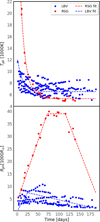 |
Fig. A.1 Photosphere temperature (top) and radius (bottom) for Type IIn/LBV (blue) and Type IIP/RSG (red) SNe. Data points are sourced from Taddia et al. (2020) and Dastidar et al. (2018). Figure adapted from Paper I. |
Utilizing these photospheric parameters, we compute the opacity for photons emitted from various regions within the remnant, thereby obtaining the attenuated γ-ray spectra.
In Paper I, absorption matrices were computed for select time points during the photosphere’s evolution, with interpolation employed to estimate γ-ray attenuation at intermediate times. In this study, we enhance our numerical approach by implementing GPU acceleration, enabling the computation of
15
absorption matrices at every output time step. This advancement eliminates the need for interpolation, thereby reducing numerical artifacts previously observed, such as those depicted in Figure 4 of Paper I.
It is important to note that our assumptions on the SN-photospheres are crucial for the resulting light curves and can differ widely between different SN. Some Type IIn SNe show photospheric emission for more then five years as in the case of SN 2017hcc (Moran et al. 2023). However, also in extreme cases, the γγabsorption will still fade considerably with time as Rph/Rsh will approach zero over time, resulting in small scattering angles and hence less and less absorption.
We plan to release the γγabsorption code freely in an upcoming publication.
A.7 EBL absorption
In addition to the photon fields discussed in Section A.6, the extragalactic background light (EBL) constitutes another significant contributor to the γγ absorption process for extragalactic sources (see e.g., Gould & Schréder 1966).
To assess the detectability of distant Type IIP and Type IIn SNe, we incorporate the effects of EBL-induced attenuation. We adopt the EBL model proposed by Finke et al. (2010) to characterize the spectral energy distribution of the EBL. Using this model, we compute the γγ optical depth of the Universe, denoted as  , for gamma-ray photons with energies corresponding to the lower and upper thresholds of various gamma-ray observatories, as a function of the source distance d. These calculations are performed utilizing the Astropy library (Astropy Collaboration 2018).
The average of the optical depths at the two energy thresholds is then used to determine the attenuation factor, which is applied to the gamma-ray flux as a multiplicative correction:
 (A.11)
This approach allows us to account for the reduction in observable gamma-ray flux due to interactions with the EBL when evaluating the prospects for detecting distant SN events. In this work, the EBL absorption becomes significantly more important as the shell-interactions can boost the gamma-ray emission significantly beyond the levels of the smooth winds we considered earlier.
Appendix B Detectability
We evaluated the detectability of the emission for various present and future gamma-ray observatories.
B.1 HE detectability
The HE gamma-ray domain is less affected by γγabsorption that observatories operation at higher energies. At the moment, the only relevant instrument in the HE gamma-ray domain is Fermi-LAT, where we already discussed the detectability in section 3.2.2 and figure 4. The detectability for Fermi is evaluated between 1 − 300 GeV.
eASTROGAMM is proposed to launch in the next decade and to observe the gamma-ray sky at slightly lower energies -here we used 100 − 1000 MeV - than Fermi-LAT with a compatible sensitivity but a considerably better angular resolution (De Angelis et al. 2017). Figure B.1 shows the detection horizon for eASTROGAM, which is compatible with Fermi-LAT’s.
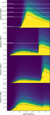 |
Fig. B.1 eASTROGAM detectability for LBV 0.1, LBV 2.0, RSG dense shell and RSG dilute shell scenarios from top to bottom. White lines indicate detected SNe explosions at their inferred distance. |
B.2 VHE-detectability
In the VHE-domain, the currently relevant instruments are the IACTs H.E.S.S., VERITAS and Magic, which all have a comparable sensitivity at higher energies and the water Cherenkov telescope HAWC.
Here, we only used the H.E.S.S.-sensitivity as a benchmark for the IACTs (see figure B.2) and integrated the spectrum between 1 − 10 TeV. For HAWC, which is more sensitive at higher energies, we used 2 − 20 TeV (see figure B.3).
In the future, CTAO will come into operation in the VHE domain and provide a superior sensitivity compared to current-generation instruments. For CTAO, we integrated or emission spectra between 1 − 20 TeV (see figure B.4).
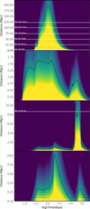 |
Fig. B.2 Same as figure B.1 but for the H.E.S.S. instrument. |
B.3 UHE-detectability
LHAASO provides us with a new window to the gamma-ray sky at energies of up to a few PeV. For the LHAASO-sensitivity plot, we integrated in the energy range of 40 − 300 TeV (see figure B.5).
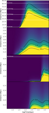 |
Fig. B.3 Same as figure B.1 but for the HAWC instrument. |
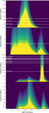 |
Fig. B.4 Same as figure B.1 but for the the planned CTAO-South observatory. |
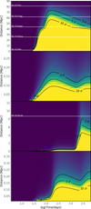 |
Fig. B.5 Same as figure B.1 but for the LHAASO observatory. |
All Tables
Time of first interaction with the shell and time until the peak in the corresponding waveband after the onset of the interaction.
All Figures
|
Fig. 1 Density profile of the CSM for the two RSG scenarios listed in Table 1. The low mass-loss case creates a more strongly diluted (yellow) shell than the high mass-loss case (purple). The dashed red lines show the density profiles. |
| In the text | |
|
Fig. 2 Total energy in CRs in units of 1051 erg for the LBV (solid) and RSG cases (dashed) as a function of time. |
| In the text | |
|
Fig. 3 Gamma-ray luminosities in the Fermi-LAT energy range (dashed) and H.E.S.S. energy range (solid) accounting for γγ absorption. Top: SNR of LBV progenitors interacting with the dense shell at different times (models as described in Table 1). The γγ absorption has ceased completely after about 200 days. Bottom: interaction of SNRs with RSG progenitors interacting with dense shells created by external photoionization. The purple case represents an upper limit in terms of shell mass, cause by a high mass-loss wind and a strong ambient photon field. The diluted case represents typical parameters for the population of RSGs (see Table 1 for details). |
| In the text | |
|
Fig. 4 Fermi detectability for LBV 0.1, LBV 2.0, and RSG high-mass and RSG low-mass scenarios, from top to bottom. The white lines indicate detected SNe explosions at their inferred distance and their overlap with the operation window of Fermi-LAT. Type IIn events are shown in the upper two panels, and Type IIP events are shown in the lower panels. |
| In the text | |
|
Fig. 5 Top panel: radio luminosity, including the effects of free-free absorption for Type IIn explosions. The green area indicates the 1σ uncertainty region for the rise time and peak radio luminosity for Type IIn SN taken from Bietenholz et al. (2021). Bottom panel: radio spectral index α of the absorbed radio flux at 4 GHz. |
| In the text | |
|
Fig. 6 Same as Figure 5, but for the RSG and Type IIP scenarios. The average of the Type IIP population is taken from Bietenholz et al. (2021). |
| In the text | |
|
Fig. 7 Absorbed thermal X-ray luminosity between 0.2 and 10 keV for Type IIn explosions (left) and Type IIP explosions (right). The gray stars indicate the measurements listed by Dwarkadas (2014). |
| In the text | |
|
Fig. 8 Top: optical light curves in the B band (398–492 nm) for an SN interaction with the two RSG shells (solid lines) and the luminosity from the SN photosphere (dotted red line). Bottom: ratio of the B- and R-band (591–727 nm) luminosities over time. |
| In the text | |
|
Fig. A.1 Photosphere temperature (top) and radius (bottom) for Type IIn/LBV (blue) and Type IIP/RSG (red) SNe. Data points are sourced from Taddia et al. (2020) and Dastidar et al. (2018). Figure adapted from Paper I. |
| In the text | |
|
Fig. B.1 eASTROGAM detectability for LBV 0.1, LBV 2.0, RSG dense shell and RSG dilute shell scenarios from top to bottom. White lines indicate detected SNe explosions at their inferred distance. |
| In the text | |
|
Fig. B.2 Same as figure B.1 but for the H.E.S.S. instrument. |
| In the text | |
|
Fig. B.3 Same as figure B.1 but for the HAWC instrument. |
| In the text | |
|
Fig. B.4 Same as figure B.1 but for the the planned CTAO-South observatory. |
| In the text | |
|
Fig. B.5 Same as figure B.1 but for the LHAASO observatory. |
| In the text | |
Current usage metrics show cumulative count of Article Views (full-text article views including HTML views, PDF and ePub downloads, according to the available data) and Abstracts Views on Vision4Press platform.
Data correspond to usage on the plateform after 2015. The current usage metrics is available 48-96 hours after online publication and is updated daily on week days.
Initial download of the metrics may take a while.