| Issue |
A&A
Volume 706, February 2026
|
|
|---|---|---|
| Article Number | A110 | |
| Number of page(s) | 9 | |
| Section | Planets, planetary systems, and small bodies | |
| DOI | https://doi.org/10.1051/0004-6361/202555863 | |
| Published online | 05 February 2026 | |
HST pre-imaging of a free-floating planet candidate microlensing event
1
Astronomical Observatory, University of Warsaw,
Al. Ujazdowskie 4,
00-478
Warszawa,
Poland
2
Korea Astronomy and Space Science Institute,
Daejeon
34055,
Republic of Korea
3
Department of Astronomy, University of Maryland,
College Park,
MD
20742,
USA
4
Code 667, NASA Goddard Space Flight Center,
Greenbelt,
MD
20771,
USA
5
Department of Physics, University of Warwick,
Coventry
CV4 7 AL,
UK
6
Department of Particle Physics and Astrophysics, Weizmann Institute of Science,
Rehovot
76100,
Israel
7
Department of Astrophysics and Planetary Sciences, Villanova University,
800 Lancaster Ave.,
Villanova,
PA
19085,
USA
8
University of Canterbury, School of Physical and Chemical Sciences,
Private Bag 4800,
Christchurch
8020,
New Zealand
9
Max-Planck-Institute for Astronomy,
Königstuhl 17,
69117
Heidelberg,
Germany
10
Department of Astronomy, Ohio State University,
140 W. 18th Ave.,
Columbus,
OH
43210,
USA
11
Department of Physics, Chungbuk National University,
Cheongju
28644,
Republic of Korea
12
National University of Science and Technology (UST),
Daejeon
34113,
Republic of Korea
13
Center for Astrophysics | Harvard & Smithsonian,
60 Garden St.,
Cambridge,
MA
02138,
USA
14
School of Science, Westlake University,
Hangzhou,
Zhejiang
310030,
China
15
Department of Astronomy, Tsinghua University,
Beijing
100084,
China
16
School of Space Research, Kyung Hee University,
Yongin,
Kyeonggi
17104,
Republic of Korea
17
Center for Cosmology and AstroParticle Physics, Ohio State University,
191 West Woodruff Ave.,
Columbus,
OH
43210,
USA
★ Corresponding author: This email address is being protected from spambots. You need JavaScript enabled to view it.
Received:
7
June
2025
Accepted:
25
October
2025
Abstract
High-cadence microlensing observations uncovered a population of very short-timescale microlensing events, which are believed to be caused by the population of free-floating planets (FFPs) roaming the Milky Way. Unfortunately, the light curves of such events are indistinguishable from those caused by wide-orbit planets. To properly differentiate both cases, one needs high-resolution observations that would allow one to resolve a putative luminous companion to the lens long before or after the event. Usually, the baseline between the event and high-resolution observations needs to be quite long (∼10 yr), hindering potential follow-up efforts. However, there is a chance to use archival data if they exist. Here, we present an analysis of the microlensing event OGLE-2023-BLG-0524, the site of which was captured in 1997 with the Hubble Space Telescope (HST). Hence, we achieve a record-breaking baseline length of 25 years. A very short duration of the event (tE = 0.346 ± 0.008 d) indicates an FFP as the explanation. Based on the finite-source effects in the light curve, we measure an angular Einstein radius value of θE = 4.78 ± 0.23 μas, suggesting a super-Earth in the Galactic disk or a sub-Saturn-mass planet in the Galactic bulge. We have not detected any potential companion to the lens with the HST data, which is consistent with the FFP origin of the event. Though we detect no potential companion to the lens in the HST imaging, we find that the HST imaging is insufficient to constrain beyond 25-48% of potential companions (depending on whether or not the occurrence rate of wide-orbit planets is correlated with the host mass); hence, we are unable to confidently confirm this event as an FFP. Despite this, our results show that archival high-resolution images should be available for many microlensing events, providing a potential new avenue to confirm FFP candidates in future observations.
Key words: gravitational lensing: micro / techniques: high angular resolution / planets and satellites: detection
© The Authors 2026
 Open Access article, published by EDP Sciences, under the terms of the Creative Commons Attribution License (https://creativecommons.org/licenses/by/4.0), which permits unrestricted use, distribution, and reproduction in any medium, provided the original work is properly cited.
This article is published in open access under the Subscribe to Open model. This email address is being protected from spambots. You need JavaScript enabled to view it. to support open access publication.
1 Introduction
Thousands of exoplanets have been identified since the first one was discovered at the end of the previous century (Mayor & Queloz 1995). The majority of them are bound to a host star. Nevertheless, many theoretical studies suggest the existence of planets that are gravitationally unattached to any star. They are also called free-floating planets, FFPs for short. Their formation can occur in various ways (but not limited to): planet-planet scattering (Rasio & Ford 1996; Lin & Ida 1997; Chatterjee, Ford, Matsumura, & Rasio 2008), interactions in stellar clusters (Spurzem et al. 2009), or post-main sequence evolution of planetary systems (Veras et al. 2011).
The introduction of high-cadence microlensing surveys has allowed us to probe this elusive population of planets, which have masses ranging from that of Earth to that of Saturn (Mróz et al. 2017; Gould et al. 2022; Sumi et al. 2023). Unlike stars and brown dwarfs, FFPs lead to very short-timescale (tE < 0.5 d) microlensing events, where tE is the Einstein timescale. Modern-day microlensing surveys such as the Optical Gravitational Lensing Experiment (OGLE; Udalski et al. 2015), Korea Microlensing Telescope Network (KMTNet, Kim et al. 2016), and Microlensing Observations in Astrophysics (MOA, Bond et al. 2001) have allowed researchers to measure angular Einstein radii, θE, together with the relative lens-source proper motion, μrel, based on the finite-source effects for FFP-like events (for the first such measurement, see Mróz et al. 2018). Thanks to such observations, we can safely rule out high proper motion as a cause for the short tE in such events, further supporting the hypothesis of planetary-mass objects. A detailed review of FFP microlensing research together with the history of the discoveries is presented by Mróz & Poleski (2024).
Even if light curves of short-timescale microlensing events seem to support the FFP hypothesis, it is hard to rule out the presence of a putative stellar companion at wide separation. It is possible that the host star will never come close enough in the sky to the source star, leaving the light curve unaffected. Fortunately, thanks to the relative lens-source proper motion, one can expect that after sufficient time the two will separate. Then, there would be a possibility to investigate the lens’s light with highresolution imaging, either with the help of adaptive optics (AO) or with space-based observatories. Such studies should reveal a putative host star to a planet if present. With a typical relative motion of 7 mas yr−1, one needs to wait for several years before such inquiry would be possible. With the help of AO on 30-m-class telescopes, one can expect around four times better resolution, and hence a four times shorter wait time (Gould 2022) compared to the current generation of telescopes, although right now we are inherently limited in our scope of tools. An example usage of AO techniques for FFP studies is presented in Mróz et al. (2024), wherein several FFP microlensing events have been investigated. Usually, such an inquiry is based on the observations obtained long after the main event. There is, however, the possibility of using pre-discovery data. There are no published applications of this alternate approach, although a similar strategy has been proposed by Bachelet et al. (2022) and Kerins et al. (2023), who suggest that the Euclid telescope can be used for pre-imagining of Roman Space Telescope fields in the Galactic bulge. Such observations can effectively extend the baseline over which one can measure the proper motion of the stars and resolve source-lens pairs, which can add crucial information for the analysis of microlensing events. Moreover, such observations would allow for a much more rapid science return from the Roman Space Telescope mission as precursor imaging data could be obtained with Euclid.
In this publication, we present an investigation of the microlensing event OGLE-2023-BLG-0524. This very shorttimescale microlensing event exhibits pronounced finite-source effects, which can be used to measure its angular Einstein radius. By pure coincidence, archival photometry from the Hubble Space Telescope (HST) is available and presents a high-resolution glimpse at the microlensing system as it was 25.55 years before the event. This is the first time ever that such observations have been used to investigate the site of a microlensing event. Due to the unprecedented time span between the HST observation and the main microlensing event, one can expect any potential putative host to the lens to be well separated in the images, allowing one to verify the hypothesis of an FFP event origin. This paper is structured as follows. In Section 2, ground-based high-cadence photometry is presented, while Section 3 is devoted to the event modeling. Then, an overview of HST data is given in the Section 4, followed by a detailed investigation that puts a limit on the putative host luminosity in Section 5. Conclusions are presented in Section 6.
2 Observations
OGLE-2023-BLG-0524 was observed toward the Milky Way bulge on a star with equatorial coordinates (α, δ)J2000 = (18°05′14.92″, −27°59′14.0″), which is located in the OGLE-IV field BLG511. The Galactic coordinates of the event are (l, b) = (2°995, −3°248). The maximum brightness was achieved on May 22,2023. The event was alerted by OGLE Early Warning System (Udalski 2003) on May 29, 2023. The OGLE survey observed the field of interest every 60 minutes during the night of the event with the 1.3 m Warsaw Telescope located at Las Campanas Observatory, Chile. The telescope is equipped with a wide field-of-view 1.4 deg2 camera (Udalski et al. 2015). Only I-band observations are available for the night of the event.
This same object was observed with the Korea Microlensing Telescope Network (KMTNet, Kim et al. 2016). KMTNet uses three telescopes located at Cerro Tololo Interamerican Observatory (KMTC), South African Astronomical Observatory (KMTS), and Siding Springs Observatory (KMTA). Each facility hosts a 1.6 m telescope with a 4 deg2 camera. During the night of the event, the KMTC facility observed a field of interest roughly every 25 minutes. While almost all of the observations are conducted in the I band, there are also a few observations in the V band taken from KMTC. Neither KMTNet AlertFinder (Kim et al. 2018b) nor KMTNet Event Finder (Kim et al. 2018a) found this event.
The photometric observations were reduced using custom pipelines by Udalski (2003) for OGLE and Albrow et al. (2009) for KMTNet. Both pipelines are based on difference image analysis (Tomaney & Crotts 1996; Alard & Lupton 1998; Wozniak 2000). Final KMTNet photometric observations were obtained with the KMTNet tender-love care pipeline (Yang et al. 2024).
Only OGLE and KMTC were able to observe the event at the peak. KMTA captured a falling wing of the light curve, while KMTS allowed us to cover the baseline of the event (for the light curve, see Figure 1). The initial examination shows that brightening is extremely short. Despite being located in a region observed at high cadence, only seven and nine observations were made during the event by OGLE and KMTC, respectively. The event shows clear signs of finite-source effects, which suppress the maximum brightness in the peak to only ~2 mag.
3 Light curve modeling
We used all available OGLE and KMT datasets in the fitting procedure, limiting ourselves only to the data collected in 2022 and 2023. The standard point-source point-lens model (PSPL) is defined using the time of maximal brightening, t0, the Einstein timescale tE = θE/μrel, and the impact parameter, u0 (expressed in terms of the Einstein radius). Finite-source effects are parametrized with ρ = θ*/θE, where θ* is the angular radius of the source star. In order to suppress any correlations between variables, parameters t* = tEρ and b0 - u0/ρ have been defined. Both variables, together with t0, ρ were used to fully define the light-curve model. During the fitting, we decided to calculate the best-fitting source flux, Fs, and blending flux, Fb, for a set of previously described parameters (u0, t0, t*, b0, ρ) to compute the χ2 value. As there is little to no information about the limb darkening coefficient at this stage, we decided to use Γ - 0.45, which should be valid for a K-type star. The Python-based library emcee (Foreman-Mackey et al. 2013) has been used to sample from the posterior and estimate uncertainties associated with the parameters. Inferred parameters together with derived ones are listed in Table 1. The light curve of the event is presented in Figure 1 along with theoretical predictions. The estimation based on the microlensing models allows us to measure the calibrated I magnitude of the source star, which is equal to  mag.
mag.
The source-to-baseline flux ratio, fs = Fs/(Fs + Fb), suggests significant blending for all datasets. This important parameter is equal to  and
and  for KMTC and OGLE datasets, respectively. Significant blending, in principle, may be attributed to the luminosity of the lens itself or a companion of the source. This rule, however, is not absolute, as the blending flux could also originate from nearby unresolved stars.
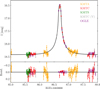 |
Fig. 1 Light curve of OGLE-2023-BLG-0524 together with the best-fit FSPL model (solid black line). All observations are scaled to the OGLE system. |
4 Hubble Space Telescope data
As the region of the event is very close to the center of the Galactic bulge, it was observed by several microlensing surveys during the last 30 years. In 1996, the MACHO collaboration observed an event that later got designated as MACHO-96-BLG-14 (Alcock et al. 2000). Following the discovery of the event, it was observed using the Wide Field and Planetary Camera 2 (WFPC2) with HST (Bennett 1997). In total, five images were taken on November 1, 1997: three in the F555W filter and two in the F814W filter (equivalents of the Johnson V and Cousins I filters, respectively). Each exposure lasted only 40 s. The WFPC2 camera consisted of four CCD detectors (numbered from 1 to 4), each with 800 × 800 pixels. The first detector (Planetary Camera, PC for short) was two times smaller than the other three, with the same number of pixels, making its resolution effectively two times higher than other detectors. In the follow-up observations of MACHO-96-BLG-14, the Planetary Camera was used to observe the main event, which was only a few arcminutes away from the star that would become the source for OGLE-2023-BLG-0524 more than 25 years later. Fortunately, HST captured the site of OGLE-2023-BLG-0524 on the second detector in the WFPC2 camera. The effective size of the pixel in the second detector is around 0″ .0996, allowing for a sub-arcsecond resolution of the event. Approximately 9333 days (25.55 yr) passed between the HST observations and the microlensing maximum.
To mitigate the chance of mistakes in the source identification, on April 26, 2025, we obtained additional two orbits of HST observations from the program GO-17834 (Terry & Mroz 2024), using the WFC3/UVIS camera. This was 1.93 years after the peak of the microlensing event. We obtained 16 × 69 sec. dithered exposures with the F814W filter and 16 × 70 sec. dithered exposures with the F606W filter using the UVIS2-C1K1C-SUB aperture. We use this sub-array to minimize the degradation effect of charge transfer efficiency (CTE) in these HST detectors. The analysis was performed using the point spread function (PSF) fitting routine hst1pass (Anderson 2022), which generates a distortion-free point source catalog of all detected stars, including the OGLE-2023-BLG-0524 source star.
Initial microlensing parameters of the event grouped by sampling parameters (upper part) and derived parameters including blending parameters for datasets (lower part).
4.1 OGLE-HST astrometric transformation
We found that the equatorial coordinates provided with the WFPC2 image deviated by around 3″ between the OGLE and HST positions. Hence, we decided to match the OGLE and HST images without the help of supplemented coordinates. In order to locate the microlensing star, we established a transformation between the coordinates on the OGLE reference image and those on the HST image. We used DOLPHOT (Dolphin 2016) to measure the position and brightness of stars on the HST image. We decided to start with a basic linear transformation realized in the form of rotation and shift. OGLE uses pixels that are 0″.26 in size, roughly 2.5 times bigger than those used in WFPC2. Hence, an additional scale parameter was added that scales the relative positions in the OGLE image to those in the HST image, resulting in a total of four parameters to fit. Then, the first image in the F814W band was selected as a grid reference. We decided to select only stars brighter than 18.5 mag to calculate the coefficients of the transformation. Each OGLE star brighter than this limit was cross-matched with the Gaia DR3 catalog (Gaia Collaboration 2023), allowing us to obtain its proper motion. We then calculated the proper-motion-corrected positions of the stars for the epoch of the HST observations. Subsequently, the coordinates of each star were transformed to a WFPC2 base, with an additional correction for a WFPC2 camera distortion (Casetti-Dinescu et al. 2021). With the established transformation, the mean distance between the nearest stars on the HST image and the transformed OGLE object was calculated and minimized using the Nelder-Mead algorithm. Finally, the transformation was established with the root mean square (RMS) error of 0.8 HST pixel. To assess the limitations of the four-parameter linear model, we tested more complex transformations, including a six-parameter linear model and a quadratic transformation. All transformations performed similarly, yielding comparable RMS errors and final object positions.
The position of the baseline star of OGLE-2023-BLG-0524 is (XO, YO) = (723.23, 351.08) in the OGLE reference image. We measured the accurate position of the source star using subtracted images in the peak, obtaining (X″O, Y″O) = (720.950 ± 0.055, 351.565 ± 0.093). After the transformation to the HST frame, we obtained coordinates (XH, YH) = (578.81, 247.59).
We do not report any problems with positional coordinates supplied with the WFC3 data. We measured the position of the event on the WFC3 dataset with supplied positional information. The coordinates of the source star on the detector are (X, Y) = (513.49 ± 0.02, 620.18 ± 0.02).
A detailed view of the vicinity of the event (on both HST datasets) is presented in Figure 2. As we can clearly see, the field is very crowded. This provides us with an easy explanation for the observed blending in the microlensing model. The source star in the OGLE reference image is composed of at least three HST counterparts separated by around 500 mas.
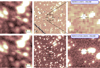 |
Fig. 2 A finding chart of OGLE-2023-BLG-0524 event viewed by OGLE (left panel) and HST (middle and right panel). The two upper right panels present archival WFPC2 data, while the two lower panels contain the modern WFPC3 dataset. A circle represents the RMS error of the linear transformation (only in the upper right panel). The Hubble images were rotated and rebinned to align the images with the northeast direction. |
4.2 HST view of the source star
We used DOLPHOT (Dolphin 2016) to measure the brightness of the source star in the WFPC2 image. The brightness in F814W and F555W filters is equal to F814W = 19.484 ± 0.023 mag and F555W = 21.112 ± 0.029 mag, respectively. Using transformations from WFPC2 to UBVRI presented in Holtzman et al. (1995), we obtained V - I = 1.670 ± 0.03 8 mag, I = 19.442 ± 0.023 mag, and V = 21.112 ± 0.029 mag. We decided against establishing our own transformation between OGLE and WFPC2 magnitudes due to the systematic effects of blending, which may cause problems for the potential transformation. Despite nearly 0.3 mag difference between the HST value and one obtained from the microlensing source estimate, both values are still consistent within 1.2σ. There is, however, a possibility that this difference in magnitudes is real and an additional  mag star is contributing to the total luminosity of the HST star. This additional light may come from the companion to the source or the luminous lens.
To obtain the magnitude of the source star in WFPC3 observations, we cross-matched WFC3 and WFPC2 images to calibrate the brightness. We fit the linear model to find the magnitude in the WFPC2 F814W filter based on the WFC3 F606W and F814W magnitudes. We found F814W′ = 19.493 ± 0.014, which is in good agreement with the WFPC2 value.
Then we proceeded with the standard method presented in Yoo et al. (2004), which allowed us to de-redden our photometry and calculate the angular radius of the source star. The red clump centroid in the vicinity of the event is ((V - I)RC, IRC) = (1.904 ± 0.015,15.296 ± 0.025) (presented in Figure 3), while dereddened values are equal to ((V - I)RC,0, IRC,0) = (1.06,14.350) (Nataf et al. 2013; Bensby et al. 2013). Assuming that the reddening toward the source is the same as that toward red clump stars, the de-reddened color of the source is equal to (V - I)0 = 0.826 ± 0.041, which can be translated to around 5300 ± 100 K and (V - K)0 = 1.842 ± 0.092 using the relation presented in Ramírez & Meléndez (2005). In order to find the final microlensing parameters, the new limb darkening value was calculated with the help of Claret & Bloemen (2011) and is equal Γ = 0.44 for observations in the I band and Γ = 0.62 for observations in the V band (for a main sequence star). We employed the colorsurface brightness relationship presented in Adams et al. (2018), allowing us to compute the angular diameter for a source. Then, new microlensing models were created: with and without a prior on the OGLE source magnitude. We assumed a Gaussian prior on Is ~ N(19.442,0.023). The comparison between parameters of both samplings together with the expected lens-source separation 25.55 years before the peak is presented in Table 2. The χ2 value for both models is around 6600 for 6359 degrees of freedom, suggesting a good fit for both models. The χ2 difference between two models is smaller than one so there is no statistical difference between them.
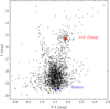 |
Fig. 3 Color-magnitude diagram showing stars in the vicinity of the event (2′ × 2′). |
Microlensing parameters computed with and without a prior on the source’s star magnitude.
5 Detectability simulations
As we derived in Section 4 (Table 2), one can expect that the source and the lens should be separated by around 129 ± 8 mas, which can be translated to 1.3 pixels on the HST image taken 25.55 years earlier. No such object was found by DOLPHOT, supporting the FFP hypothesis. Nevertheless, the FFP hypothesis may not be correct, as the faint star may be undetectable on the HST image due to the presence of a nearby field star. In order to investigate limits on a possible companion, we decided to simulate its detectability in the HST images. The nearest object, located just five pixels away, is actually composed of two stars separated by only one pixel. This stellar asterism can complicate the detection problem, as one expects that detectability will not be independent of the source-lens angle.
This section is structured as follows. In Section 5.1, a theoretical description of the detectability simulations is presented. Subsequently, three subsections are devoted to particular detection cases. In Section 5.2, we use tools described in the first subsection to model the actual HST image. Then, in Sections 5.3 and 5.4 we test the detectability limits of putative host stars.
5.1 Theoretical introduction
Let us denote the total photons counted in pixel (X, Y) as N(X, Y), while the mean number of theoretically predicted counts is designated F(X, Y). The simulation begins with the initialization of the 12 × 12 grid (which covers roughly 1″ × 1″). Then, N(X, Y) is sampled from a Poisson distribution with rate F(X, Y). At the end, we add additional Gaussian noise, σ, to each pixel, which simulates the readout noise. For a given separation between stars, s, and their magnitude difference, m, we fit two models: the single-star model and the double-star model. We performed fitting with the Nelder-Mead algorithm using χ2 as a loss function:
 (1)
(1)
We decided to use the TinyTim (Krist et al. 2011) PSF library to simulate PSFs for all models. This particular approach is better than DOLPHOT, as TinyTim numerically computes the PSF rather than relying on simple analytical approximations. As the size of the PSF is determined by the position on the detector, we only need to fit the position of the star. After using maximally subsampled PSF, we performed the linear interpolation with re-binning, followed by a convolution with a charge diffusion kernel, which is presented in the TinyTim manual1. In the single-star model, we include only one star with a constant sky value. We have four parameters in total: the position (X1,Y1), the total luminosity of the star, F1, and the background, B. In the double-star model, we added an additional star with three more parameters: (X2, Y2) and F2. In general, one can write that
 (2)
(2)
where we have summation over the number of stars and where PSF denotes the point spread function obtained from TinyTim.
5.2 Modeling the HST image
As we noted in previous sections, the source star is much fainter in the F555W filter than in the F814W one. This is reflected by the higher signal-to-noise ratio (S/N) in the F814W filter, which is around 34 compared to 22 in the case of F555W. In order to maximize the chances of detection, we decided to work on images in the F814W filter only. Observations have been made in “15” gain mode, indicating a gain value of around ~14.5 and a readout noise of ~7.84 (taken from WFPC2 manual2. A 12 × 12 cutout was created from the image, which contains the source star and nearest neighbor clump of stars.
We know that the DOLPHOT was able to detect only three stars in the cutout. Hence, it was decided to fit four and three-star TinyTim PSF models. With the three-star model, we should obtain a similar fitting to the DOLPHOT model. With the four-star model, we can search for the putative companion to the lens. The three-star model achieved χ2 = 140.4 and χ2 = 150.4 for 132 and 133 degrees of freedom on the first and second images, respectively (two and one pixels on the first and second images, respectively, were reported to be bad, and hence they were not used in the analysis). The four-star model is not able to improve the score beyond ∆χ2 = 2, so no significant detection is reported. Images used in the inquiry together with residuals from the three-star model are presented in Figure 4. The source star’s brightness was measured and is equal to Fs = 2125.6 e−, while the background is equal to around B = 20.6e−. Those two values were then used to perform simulations.
5.3 Detecting putative host star
We can use the HST image to perform injection-and-recovery simulations and find out whether the putative host star is detectable. Such simulations are composed of two steps: injection of the putative star into a simulated image and fitting a model to recover the injected object. First, we need to create artificial images containing two stars (source and putative companion to the lens), each with dimensions of 12 × 12. Then, we fit a single-star model and a double-star model, and compare the goodness of fit for both models.
To create an artificial population of host stars, we need to specify the relative host-source separation and the luminosity distribution of the stars. We used the distribution of separations from our Bayesian microlensing model (the second column in Table 2). We assumed that the total luminosity of stars was constant and equal to I = 19.484. While the total brightness of stars was constant, the relative magnitude difference was sampled from the uniform distribution of ∆m ~ U(0,5).
In total 2 ∙ 105 simulations were performed. The relative angle between the stars was randomized. We decided to use a BIC score to determine which model is preferred. The BIC score is defined by the formula
 (3)
(3)
where k is the number of parameters, while n denotes the size of our image in pixels (here 144; we use a 12 × 12 grid). If the BIC score for a two-star model (BIC2) is lower than for the onestar model (BIC1), we would prefer the two-star model. Usually, one requires a difference of about a dozen in the BIC scores to decide which model is preferred. However, we decided not to raise the bar for detection, so the lower BIC score for the doublestar model would suffice. If the double-star model is better, we can write that
 (4)
(4)
as the double-star model has three more parameters than the single-star model. We defined the difference in χ2 scores as  , where
  and
and  denote X scores for the single and double model, respectively. Hence, we require ∆χ2 > 3 ln 144 ≈ 14.9 difference to report a detection. Simulated ∆χ2 differences between a two-star model and a one-star model are presented in Figure 5. Aditionally, a 1σ interval has been overplotted. This intrinsic uncertainty is associated with a different initialization of the grid and different separations.
Usually, one would like to assess whether stars with luminosity above some threshold are detectable or not. This division becomes blurry due to the very low S/N of the source star, which prompted us to establish another form of detectability criterion. Let ∆mt be the brightness difference such that we detect 95% of potential host-source pairs whose brightness differs by less than ∆mt. Then, the ∆mt value can be used to calculate the corresponding magnitude of the host star, mt, as we know the total luminosity of stars. Even if the value ∆mt is clearly defined, it depends on the choice of our prior on the luminosity and separation. While the separations are modeled according to the posterior distribution of separations from the microlensing model, the distribution of the relative magnitudes is described in a somewhat artificial manner. Nevertheless, as we were mainly concerned with simple estimation, we settled on the simple uniform distribution, as was noted in the previous paragraph.
Using the aforementioned simulations, we established that ∆mt = 2.17 mag, which translates to a limiting magnitude of mt = 21.74 mag. Hence, 95% of putative hosts brighter than 21.74 mag should be detected. A stricter limit was also calculated at the 99.7% detection ratio (3σ), which corresponds to ∆mt = 0.94 mag and mt = 20.76 mag. The dependence between the observable luminosity of the star and the detection probability is presented in Figure 6.
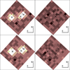 |
Fig. 4 F814W residuals together with images used for the fitting. Each star is marked with a number according to its luminosity (from darkest to brightest). Microlensing source is the brightest and is denoted with the number “3”. Images are rotated to align with the northeast direction. |
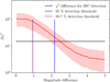 |
Fig. 5 Simulated ∆χ2 differences (with a 1σ interval) plotted against the magnitude difference between both stars. Vertical lines indicate 2σ and 3σ detection thresholds. |
5.4 The percentage of putative host stars that we can detect
In the end, we decided to simulate an artificial population of stars that would represent the potential population of a putative host stars. The masses of the stars were sampled from the Chabrier mass function (Chabrier 2003), while proper motions and distances were obtained using the Galactic model presented in Batista et al. (2011). Then, the mass-I-band and the mass-V-band luminosity relationships presented in Pecaut & Mamajek (2013) were used to obtain the observable brightness in the F814W filter with the transformation from Holtzman et al. (1995). We assumed that the extinction is proportional to the total integrated density of the gas in the line of sight. The probability was assigned to each star based on the geocentric relative lens-source proper motion value, μrel,
 (5)
(5)
where μ and σ represent the mean and standard deviation of geocentric proper motion obtained from the microlensing curve and presented in Table 2.
We decided to include an additional term in the probability that is related to the mass of the host star P ∝ Mn. Several studies have found that the likelihood that a given star hosts a planetary system is a function of the mass of the star (see Mulders 2018 for a review on the host star properties). We decided to use the results presented in Johnson et al. (2010), in which a nearly linear dependency on the host-star mass was found (n = 1). We also decided to include in the analysis a population of host stars with no probability dependence on the mass (n = 0) following Mróz et al. (2024).
We took 107 samples in total from the Galactic model. Subsequently, we selected 5 ∙ 104 with the “sampling, importance, resampling” procedure according to the obtained probabilities. Then, we performed detectability simulations for resampled objects according to the previously outlined procedure. This allowed us to model the detectability of putative hosts with proper priors on the separations and magnitudes. It was determined that for n = 0 only 25% of stars should be detected. For n = 1 this number increases to around 48%. Hence, predicted detection ratios are comparable to values presented in Mróz et al. (2024). Moreover, the detection probability dependence on the distance to the lens was determined and is presented in Figure 7.
The difference between the two considered populations of stars indicates that the final probability strongly depends on the correlation between the wide-orbit planet occurrence rate and the host mass. If such a correlation were to exist, we would be more likely to detect the host in the high-resolution images. For example, a study by Nunota et al. (2024) indicates that such a correlation might indeed exist for planets located at wide separations that are probed by microlensing, although there are still large uncertainties. To further investigate how our results depend on other assumptions of the model (e.g., spatial distribution and kinematics of lenses and sources, mass function), we decided to test an alternative Galactic model. We used the genulens model (Koshimoto et al. 2021 ; Koshimoto & Ranc 2022), as it is able to correctly reproduce the distribution of timescales observed in microlensing surveys. We followed the same steps as were described in the previous paragraph. We generated and then subsampled the population of microlensing stars to finaly simulate the detectability of such population. We estimated that around 33% of putative host stars in the genulens model should be detected. These results are consistent with findings described in previous paragraph. We can hence safely rule out around 30% of possible host stars.
Despite a much longer baseline, no strict limits can be imposed. First of all, optical observations (even those in the I band) cannot detect most main sequence stars with such a short exposure time. To understand the limitations associated with the detections, let us consider the simulated distribution of F814W magnitudes presented in Figure 8. Based on the HST images, we conclude that stars fainter than 24 mag are not detected on images in F814W filter. We assume that this particular value is a limiting magnitude (fainter stars are impossible to detect no matter whether they are crowded or not). This assumption allows us to estimate the fraction of putative host stars that should be detected without any other obscuring factors (such as crowding). Although in the n = 1 case, we would be able to recover a significant part of the population (around 76%), for the n = 0 case we would be able to recover only 50% of those. Hence, such a shallow image is not able to provide any conclusive answer with regard to the event’s nature. In general, near-infrared observations with a telescope such as JWST would be able to obtain much stricter limits than the presented WFPC2 analysis.
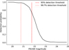 |
Fig. 6 Dependence between the detection probability and the observed F814W magnitude with the detection thresholds overplotted. Results are marginalized over the distribution of separations. |
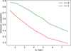 |
Fig. 7 Dependence between the detection probability and the distance to the lens, DL. Two populations are considered: no probability dependence on mass (n = 0) and P ∝ M (n = 1). Results are marginalized over the distribution of magnitudes and separations. |
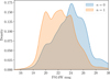 |
Fig. 8 Probability density of F814W host star magnitudes. Two populations are considered: n = 0 and n = 1. |
6 Conclusions
As was proved in the previous section, it is highly unlikely that the source star is contaminated with additional blending from the putative lens host (even if the total change in flux is negligible). Hence, in the final analysis, we decided to use the prior on the lens’s I magnitude (second column in Table 2). The final mass of the lens can be computed with
 (6)
(6)
where κ = 8.144 mas M−1. Under the assumption that the lens is located in the Galactic disk (e.g., πrel = 0.1 mas), one obtains M = 9.3 M⊕. If the lens is located in the Galactic bulge (e.g., πrel = 0.016 mas), one obtains M = 58 M⊕ (0.6 Saturn’s mass).
OGLE-2023-BLG-0524 presents an interesting case, for which archival photometric measurements allowed us to directly obtain the color of the source star. If no such observations had been made, the color would have been estimated from the V-band measurements during the peak. However, due to the very short effective timescale of the event, V-band measurements are very limited (only one measurement from the KMTC site). Despite the fact that the OGLE-2023-BLG-0524 event has a longer Einstein timescale than other FFP-candidate events observed up to this day, the source-star crossing time, t*, is one of the shortest that have been measured. In this publication we navigated the issue with the help of HST data; however, many similar microlensing events will lack color estimation. This may pose a significant problem in the future as the θE determination is heavily dependent on the source’s color (Mróz et al. 2020).
Hopefully, next-generation telescopes like the Extremely Large Telescope (ELT) would allow us to mitigate such issues. Let us consider an event similar to OGLE-2023-BLG-0524. Assuming full width at half maximum (FWHM) equal to  mas on the MICADO instrument (K band, Davies et al. 2021), three years would suffice for the source-lens system to separate to the extent of the FWHM width. At the same time, a 39 m mirror would allow one to detect much fainter hosts and enable the determination of the source’s color.
The detectability simulations allow us to impose some constraints on the putative host star population. Despite a nearly 25-year baseline, we are able to reject only around 25% of potential stars. Hence, these archival HST observations turned out to have insufficient depth to conduct decisive detectability simulations. We are able to constrain the maximum luminosity of the putative host star to around 21.74 mag in the I band at a 95% confidence interval. However, our work points out that such archival observations create a viable way of verifying the freefloating origin of microlensing events. We hope that telescopes such as JWST, Euclid, or the Nancy Roman Space Telescope will provide better opportunities in the future for such inquiries.
At the end, we estimated the number of microlensing events with such archival HST data. We used OGLE IV data presented in Mróz et al. (2019), obtaining the event rate density Γdeg2 = 113.9 yr−1deg−2 for the BLG511 OGLE-IV field. If we use all three WFPC2 detectors (80″ × 80″ each), we expect around 0.17 events per year. Hence, many events should be present in the archival HST images, similar to the one used in this study. We conducted a search for events among the OGLE IV database that could have been covered by this particular HST dataset. One event (OGLE-2017-BLG-0960) is located just a few pixels away from the edge of the detector. Nevertheless, such searches for microlensing objects across archival HST datasets offer the possibility of getting a better view of the microlensing system, as it was many years before the event.
Acknowledgements
We would like to thank Tomasz Bulik for the discussion. This research was funded in part by the National Science Centre, Poland, grant OPUS 2021/41/B/ST9/00252 awarded to P.M. S.T. was supported in part by NASA under award number 80GSFC21M0002. This research is based on observations made with the NASA/ESA Hubble Space Telescope obtained from the Space Telescope Science Institute, which is operated by the Association of Universities for Research in Astronomy, Inc., under NASA contract NAS 5-26555. This work presents results from the European Space Agency (ESA) space mission Gaia. Gaia data are being processed by the Gaia Data Processing and Analysis Consortium (DPAC). Funding for the DPAC is provided by national institutions, in particular the institutions participating in the Gaia MultiLateral Agreement (MLA). The Gaia mission website is https://www.cosmos.esa.int/gaia. The Gaia archive website is https://archives.esac.esa.int/gaia. This research has made use of the KMTNet system operated by the Korea Astronomy and Space Science Institute (KASI) at three host sites of CTIO in Chile, SAAO in South Africa, and SSO in Australia. Data transfer from the host site to KASI was supported by the Korea Research Environment Open NETwork (KREONET). This research was supported by KASI under the R&D program (project No. 2025-1-830-05) supervised by the Ministry of Science and ICT. W.Zang, H.Y., S.M., R.K., J.Z., and W.Z. acknowledge support by the National Natural Science Foundation of China (Grant No. 12133005). W.Z. acknowledges the support from the Harvard-Smithsonian Center for Astrophysics through the CfA Fellowship. J.C.Y. and I.-G.S. acknowledge support from U.S. NSF Grant No. AST-2108414. Work by C.H. was supported by the grants of National Research Foundation of Korea (2019R1A2C2085965 and 2020R1A4A2002885). J.C.Y. acknowledges support from a Scholarly Studies grant from the Smithsonian Institution.
References
- Adams, A. D., Boyajian, T. S., & Von Braun, K. 2018, MNRAS, 473, 3608 [NASA ADS] [CrossRef] [Google Scholar]
- Alard, C., & Lupton, R. H. 1998, ApJ, 503, 325 [Google Scholar]
- Albrow, M. D., Horne, K., Bramich, D. M., et al. 2009, MNRAS, 397, 2099 [NASA ADS] [CrossRef] [Google Scholar]
- Alcock, C., Allsman, R. A., Alves, D. R., et al. 2000, ApJ, 541, 734 [Google Scholar]
- Anderson, J. 2022, Instrument Science Report WFC3 2022-5 [Google Scholar]
- Bachelet, E., Specht, D., Penny, M., et al. 2022, A&A, 664, A136 [NASA ADS] [CrossRef] [EDP Sciences] [Google Scholar]
- Batista, V., Gould, A., Dieters, S., et al. 2011, A&A, 529, A102 [NASA ADS] [CrossRef] [EDP Sciences] [Google Scholar]
- Bennett, D. 1997, Snapshot Survey of Microlensed Source Stars (USA: HST Proposal ID 7431. Cycle 7) [Google Scholar]
- Bensby, T., Yee, J. C., Feltzing, S., et al. 2013, A&A, 549, A147 [NASA ADS] [CrossRef] [EDP Sciences] [Google Scholar]
- Bond, I. A., Abe, F., Dodd, R. J., et al. 2001, MNRAS, 327, 868 [Google Scholar]
- Casetti-Dinescu, D. I., Girard, T. M., Kozhurina-Platais, V., et al. 2021, PASP, 133, 064505 [Google Scholar]
- Chabrier, G. 2003, PASP, 115, 763 [Google Scholar]
- Chatterjee, S., Ford, E. B., Matsumura, S., & Rasio, F. A. 2008, ApJ, 686, 580 [NASA ADS] [CrossRef] [Google Scholar]
- Claret, A., & Bloemen, S. 2011, A&A, 529, A75 [NASA ADS] [CrossRef] [EDP Sciences] [Google Scholar]
- Davies, R., Hörmann, V., Rabien, S., et al. 2021, The Messenger, 182, 17 [NASA ADS] [Google Scholar]
- Dolphin, A. 2016, Astrophysics Source Code Library [record ascl:1608.013] [Google Scholar]
- Foreman-Mackey, D., Hogg, D. W., Lang, D., & Goodman, J. 2013, PASP, 125, 306 [Google Scholar]
- Gaia Collaboration (Vallenari, A., et al.) 2023, A&A, 674, A1 [NASA ADS] [CrossRef] [EDP Sciences] [Google Scholar]
- Gould, A. 2022, arXiv e-prints [arXiv:2209.12501] [Google Scholar]
- Gould, A., Jung, Y. K., Hwang, K.-H., et al. 2022, JKAS, 55, 173 [NASA ADS] [Google Scholar]
- Holtzman, J. A., Burrows, C. J., Casertano, S., et al. 1995, PASP, 107, 1065 [NASA ADS] [CrossRef] [Google Scholar]
- Johnson, J. A., Aller, K. M., Howard, A. W., & Crepp, J. R. 2010, PASP, 122, 905 [Google Scholar]
- Kerins, E., Bachelet, E., Beaulieu, J.-P., et al. 2023, arXiv e-prints [arXiv:2306.10210] [Google Scholar]
- Kim, S.-L., Lee, C.-U., Park, B.-G., et al. 2016, JKAS, 49, 37 [Google Scholar]
- Kim, D. J., Kim, H. W., Hwang, K. H., et al. 2018a, AJ, 155, 76 [NASA ADS] [CrossRef] [Google Scholar]
- Kim, H.-W., Hwang, K.-H., Shvartzvald, Y., et al. 2018b, arXiv e-prints [arXiv:1806.07545] [Google Scholar]
- Koshimoto, N., & Ranc, C. 2022, https://doi.org/10.5281/zenodo.6869520 [Google Scholar]
- Koshimoto, N., Baba, J., & Bennett, D. P. 2021, ApJ, 917, 78 [NASA ADS] [CrossRef] [Google Scholar]
- Krist, J. E., Hook, R. N., & Stoehr, F. 2011, SPIE Conf. Ser., 8127, 81270J [Google Scholar]
- Lin, D. N. C., & Ida, S. 1997, ApJ, 477, 781 [NASA ADS] [CrossRef] [Google Scholar]
- Mayor, M., & Queloz, D. 1995, Nature, 378, 355 [Google Scholar]
- Mróz, P., & Poleski, R. 2024, Exoplanet Occurrence Rates from Microlensing Surveys (Cham: Springer International Publishing), 1 [Google Scholar]
- Mróz, P., Udalski, A., Skowron, J., et al. 2017, Nature, 548, 183 [Google Scholar]
- Mróz, P., Ryu, Y. H., Skowron, J., et al. 2018, AJ, 155, 121 [CrossRef] [Google Scholar]
- Mróz, P., Udalski, A., Skowron, J., et al. 2019, ApJS, 244, 29 [Google Scholar]
- Mróz, P., Poleski, R., Han, C., et al. 2020, AJ, 159, 262 [CrossRef] [Google Scholar]
- Mróz, P., Ban, M., Marty, P., & Poleski, R. 2024, AJ, 167, 40 [CrossRef] [Google Scholar]
- Mulders, G. D. 2018, arXiv e-prints [arXiv:1805.00023] [Google Scholar]
- Nataf, D. M., Gould, A., Fouqué, P., et al. 2013, ApJ, 769, 88 [Google Scholar]
- Nunota, K., Koshimoto, N., Suzuki, D., et al. 2024, ApJ, 967, 77 [Google Scholar]
- Pecaut, M. J., & Mamajek, E. E. 2013, ApJS, 208, 9 [Google Scholar]
- Ramírez, I., & Meléndez, J. 2005, ApJ, 626, 465 [Google Scholar]
- Rasio, F. A., & Ford, E. B. 1996, Science, 274, 954 [Google Scholar]
- Spurzem, R., Giersz, M., Heggie, D. C., & Lin, D. N. C. 2009, ApJ, 697, 458 [Google Scholar]
- Sumi, T., Koshimoto, N., Bennett, D. P., et al. 2023, AJ, 166, 108 [NASA ADS] [CrossRef] [Google Scholar]
- Terry, S., & Mroz, P. 2024, Confirming Serendipitous Microlens Host Detections with New and Archival HST Imaging, HST Proposal. Cycle 32, ID. #17834 [Google Scholar]
- Tomaney, A. B., & Crotts, A. P. S. 1996, AJ, 112, 2872 [Google Scholar]
- Udalski, A. 2003, AcA, 53, 291 [NASA ADS] [Google Scholar]
- Udalski, A., Szymanski, M. K., & Szymanski, G. 2015, AcA, 65, 1 [Google Scholar]
- Veras, D., Wyatt, M. C., Mustill, A. J., Bonsor, A., & Eldridge, J. J. 2011, MNRAS, 417, 2104 [Google Scholar]
- Wozniak, P. R. 2000, AcA, 50, 421 [Google Scholar]
- Yang, H., Yee, J. C., Hwang, K.-H., et al. 2024, MNRAS, 528, 11 [NASA ADS] [CrossRef] [Google Scholar]
- Yoo, J., DePoy, D. L., Gal-Yam, A., et al. 2004, ApJ, 603, 139 [Google Scholar]
All Tables
Initial microlensing parameters of the event grouped by sampling parameters (upper part) and derived parameters including blending parameters for datasets (lower part).
Microlensing parameters computed with and without a prior on the source’s star magnitude.
All Figures
|
Fig. 1 Light curve of OGLE-2023-BLG-0524 together with the best-fit FSPL model (solid black line). All observations are scaled to the OGLE system. |
| In the text | |
|
Fig. 2 A finding chart of OGLE-2023-BLG-0524 event viewed by OGLE (left panel) and HST (middle and right panel). The two upper right panels present archival WFPC2 data, while the two lower panels contain the modern WFPC3 dataset. A circle represents the RMS error of the linear transformation (only in the upper right panel). The Hubble images were rotated and rebinned to align the images with the northeast direction. |
| In the text | |
|
Fig. 3 Color-magnitude diagram showing stars in the vicinity of the event (2′ × 2′). |
| In the text | |
|
Fig. 4 F814W residuals together with images used for the fitting. Each star is marked with a number according to its luminosity (from darkest to brightest). Microlensing source is the brightest and is denoted with the number “3”. Images are rotated to align with the northeast direction. |
| In the text | |
|
Fig. 5 Simulated ∆χ2 differences (with a 1σ interval) plotted against the magnitude difference between both stars. Vertical lines indicate 2σ and 3σ detection thresholds. |
| In the text | |
|
Fig. 6 Dependence between the detection probability and the observed F814W magnitude with the detection thresholds overplotted. Results are marginalized over the distribution of separations. |
| In the text | |
|
Fig. 7 Dependence between the detection probability and the distance to the lens, DL. Two populations are considered: no probability dependence on mass (n = 0) and P ∝ M (n = 1). Results are marginalized over the distribution of magnitudes and separations. |
| In the text | |
|
Fig. 8 Probability density of F814W host star magnitudes. Two populations are considered: n = 0 and n = 1. |
| In the text | |
Current usage metrics show cumulative count of Article Views (full-text article views including HTML views, PDF and ePub downloads, according to the available data) and Abstracts Views on Vision4Press platform.
Data correspond to usage on the plateform after 2015. The current usage metrics is available 48-96 hours after online publication and is updated daily on week days.
Initial download of the metrics may take a while.