| Issue |
A&A
Volume 706, February 2026
|
|
|---|---|---|
| Article Number | A217 | |
| Number of page(s) | 11 | |
| Section | Galactic structure, stellar clusters and populations | |
| DOI | https://doi.org/10.1051/0004-6361/202556502 | |
| Published online | 16 February 2026 | |
LRPayne: Stellar parameters and abundances from low-resolution spectra
1
Dipartimento di Fisica e Astronomia, Universitá di Padova,
vicolo dell’Osservatorio 2,
35122
Padova,
Italy
2
INAF – Osservatorio Astronomico di Padova,
vicolo dell’Osservatorio 5,
35122
Padova,
Italy
★ Corresponding author: This email address is being protected from spambots. You need JavaScript enabled to view it.
; This email address is being protected from spambots. You need JavaScript enabled to view it.
Received:
18
July
2025
Accepted:
7
November
2025
Abstract
Aims. This paper introduces LRPayne, a novel algorithm designed for the efficient determination of stellar parameters and chemical abundances from low-resolution optical spectra, with a primary focus on data from large-scale galactic surveys such as WEAVE.
Methods. LRPayne employs a model-driven approach, utilising a fully connected artificial neural network (ANN), trained on a library of 70 000 synthetic stellar spectra generated using iSpec with 1D model atmospheres and the Turbospectrum synthesis code. We trained the network to predict normalized flux given stellar labels (Teff, log(g), [Fe/H], vmic, vmax, and v sin i, plus 24 individual elemental abundances). We subsequently derived stellar parameters from observed spectra by finding the best-fit synthetic spectrum from the ANN using a χ2 minimisation technique. The method operates on spectra degraded to a resolution of R=5000 covering the 42006900 Å wavelength range.
Results. Internal accuracy tests on synthetic spectra show a median interpolation error of less than 0.13% for 90% of the validation sample. The method accurately recovers most of the input labels from synthetic spectra, even at a signal-to-noise ratio (S/N) of 20, with some expected challenges for elements such as Li, K, and N. Validation on the observed spectra of 25 Gaia FGK benchmark stars and 42 metal-poor stars reveals good agreement with the literature values. For the stellar parameters, the mean differences are 22±87 K for Teff, 0.19±0.23 dex for log(g), and 0.01±0.17 dex for [Fe/H]. Abundances for elements such as Na, Mg, Si, and most Fe-peak elements (Cr, Ni, V, and Sc) are well-recovered. We note challenges for oxygen, manganese in metal-rich giants, aluminium in metal-poor stars and dwarfs, and deriving log g in hot metal-poor dwarfs, partly due to non-local thermodynamic equilibrium effects and line characteristics.
Conclusions. LRPayne demonstrates the possibility of extracting precise stellar parameters and chemical abundances from a large number of low-resolution spectra. Its strong performance across different kinds of stars makes it well-suited for current and future large surveys. The abundance results from LRPayne will be very useful for studying stellar nucleosynthesis and the chemical evolution of our Galaxy on a large scale.
Key words: methods: data analysis / techniques: spectroscopic / surveys / stars: abundances / stars: fundamental parameters
© The Authors 2026
 Open Access article, published by EDP Sciences, under the terms of the Creative Commons Attribution License (https://creativecommons.org/licenses/by/4.0), which permits unrestricted use, distribution, and reproduction in any medium, provided the original work is properly cited.
This article is published in open access under the Subscribe to Open model. This email address is being protected from spambots. You need JavaScript enabled to view it. to support open access publication.
1 Introduction
The era of large-scale spectroscopic surveys has transformed stellar astrophysics, thanks to their unprecedented data volumes. Current and upcoming ground-based surveys such as the WEAVE1 (Dalton et al. 2012; Jin et al. 2024), 4MOST2 (de Jong et al. 2019), DESI3 (DESI Collaboration 2016), and the completed APOGEE4 (Majewski et al. 2017), Gaia-ESO (Gilmore et al. 2012), RAVE5 (Steinmetz et al. 2006), LAMOST6 (Cui et al. 2012), and GALAH7 (De Silva et al. 2015) surveys collectively target 106−107 stars, providing an unparalleled view of Galactic structure, stellar populations, and chemical evolution. For instance, WEAVE alone is expected to observe roughly 5 million objects over its operational lifetime, while 4MOST aims to obtain spectra for more than 10 million objects across multiple Galactic components. Special mention should be given to the Gaia BP/RP Montegriffo et al. (2023) and Euclid NISP8 Euclid Collaboration: Jahnke et al. (2025) missions, which have or will collect millions of spectra - mostly at extremely low resolutions - along with the Gaia RVS9 mission Gaia Collaboration (2023), which will observe a few million spectra at medium resolution. Though traditional spectroscopic analysis methods are generally accurate, they are not scalable to handle such enormous datasets within reasonable time frames and computational power. Therefore, machine learning techniques have emerged as the natural solution to these challenges. Recent years have witnessed a surge in the development and application of automated techniques to stellar spectroscopy. Notable examples include The Cannon (Ness et al. 2015), which has popularised the use of data-driven models for large-scale spectroscopic analysis, StarNet (Fabbro et al. 2018), which employs convolutional neural networks for stellar parameter determination, and The Payne (Ting et al. 2019), which introduces a model-driven approach using synthetic spectra to train neural networks for full spectral fitting.
Although these efforts demonstrate the huge potential of machine learning in stellar spectroscopy, most focus primarily on high-resolution spectroscopic data (R ≥ 20000). However, the landscape of upcoming surveys reveals a different reality: the vast majority of spectroscopic data will be obtained at low to moderate resolution (R ~ 2000-10 000). This shift towards lower resolution is driven by practical considerations: higher spectral multiplexing capabilities, increased survey efficiency, and the ability to observe fainter targets and hence probe larger volumes within reasonable integration times. Surveys such as WEAVE’s low-resolution (LR) mode (R ~ 5000), 4MOST's low-resolution spectroscopy (R ~ 4000-7700), and similar modes in other facilities will generate the bulk of future spectroscopic data.
A major scientific goal for the development of automated methods is to extract detailed chemical information about the vast number of stars observed by these surveys. Reliable abundance estimation from low-resolution spectra will make it possible to investigate stellar nucleosynthesis and trace the chemical enrichment of the Milky Way across different Galactic components, shedding light on the processes involved in their formation.
In this paper, we present LRPayne10, a machine learning algorithm specifically designed for the efficient determination of stellar parameters and chemical abundances from low-resolution optical spectra. Our approach builds upon the model-driven philosophy of The Payne but incorporates several tweaks tailored to the low-resolution regime. The paper is structured as follows: Section 2 describes our methodology, including the observed data used for validation, the synthetic spectral library, and the neural network architecture. Section 3 presents our results, including internal accuracy tests on synthetic spectra and validation using benchmark stars and metal-poor stars with well-established parameters from the literature. We conclude with a summary of our main findings and discuss the implications for large-scale spectroscopic surveys.
2 Methods
2.1 Architecture
For the algorithm, we adopted the model-driven approach of The Payne11 but with a few modifications. The Payne method is a machine learning-based approach to full spectral fitting used for the determination of stellar labels. At its core, The Payne uses a fully connected artificial neural network (ANN) as a spectral interpolator to estimate the flux values at each wavelength point given a set of stellar parameters. This is a suitable solution for the analysis of low-resolution spectra because it can simultaneously fit multi-dimensional labels by using the whole spectrum. This approach also allows direct estimation of the uncertainties on the derived parameters, as well as characterisation of the covariances between different labels arising due to line blending.
In Ting et al. (2019), they employ a fully connected four-layer ANN consisting of an input layer, two hidden layers, and an output layer. The number of neurons in the input and output layers is dictated by the number of parameters used for the analysis (hereafter referred to as labels) and the number of wavelength points in the final output model (hereafter referred to as pixels). However, the number of neurons in the hidden layers and the number of layers itself can vary depending on the complexity of the dataset. In Ting et al. (2019), the authors determine that two hidden layers with 300 neurons each strike a good balance, ensuring reliable interpolation without the risk of overfitting.
In our case, after extensive testing, we settled on a five-layer model in which each of the three hidden layers has 200 neurons. Between the first four layers, we used a Leaky Rectified Linear Unit (LeakyReLU) activation function ( Leak yReLU ( x) = max(0, x) + slope * min(0, x)) and a sigmoid activation function (s(x) = (1 + e−x)−1) between the last hidden layer and the output layer. The LeakyReLU function helps to prevent the vanishing-gradient problem, in which the values of the weights gbecome quite small, leading to extremely slow convergence or stagnation of the training. The sigmoid function ensures that the output values are always between 0 and 1, which is necessary for a normalised spectrum. Figure 1 illustrates the complete workflow and architecture of the neural network, with the model implemented in TensorFlow (Abadi et al. 2015).
2.2 Training
To train the neural network, we used a sample of 70000 synthetic spectra, which we divided into a training and validation set with an 80-20% split. The model uses the stochastic optimizer ADAM (Adaptive Moment Estimation) (Kingma & Ba 2014) with an initial learning rate of 0.001 and a learning rate scheduler that reduces the rate by a factor of 0.5 for every ten steps of unchanged loss. For the loss, we used the mean absolute percentage error to assist with the gradient descent. We performed the training in two steps within each iteration: forward and backward propagation. Before the start of the first forward propagation, we assigned random weights to each layer. This was achieved using layer initialisers, which are a set of instructions that define how these random weights are set (in our case, we used the He-initialiser (He et al. 2015) for all three hidden layers). Upon initialisation, the ANN uses the input (taken from training set) and randomised weights to calculate a prediction that is compared with the desired output to obtain the loss. Then, in the backward propagation step, this loss is used to calculate the gradient with respect to each weight and bias, which is then updated to a new value depending on the type of optimiser and learning rate used. The new weights are then used for the next forward propagation, and so on. The ANN uses the validation sample to keep a track of the gradient descent to avoid over-fitting, along with serving as a generalisation test. As the weights of the ANN are optimised using training data, testing the optimisation on an unseen validation sample provides the user with an unbiased estimate of the model’s performance on unseen generalised data.
Once we had a trained model, we input a random set of parameters to obtain a normalised spectrum, referred to as the constructed spectrum. We used the curve_fit routine within the SciPy package of Python to perform a simple χ2 minimisation between the constructed spectrum and the observed spectrum to determine the best-fit stellar parameters. To ensure that curve_fit did not fall within local minima, we adopted a tolerance of 10−10, which provided a good compromise between reliable convergence and computation time.
2.3 Masking
A major problem that arises with using neural network trained on synthetic models to fit observed spectrum is the inability of the network to reproduce any particular observed spectrum perfectly. This is likely due to incomplete and approximate treatment of the physics relevant to stellar atmospheres (such as NLTE and 3D effects), incomplete linelists, and inaccurate atomic parameters. Therefore, we followed the method described in Ting et al. (2019), masking bad pixels when fitting. To this end, we compared the high S/N solar observed spectrum with the constructed spectrum (constructed using solar values for the labels) and masked any pixel that showed a deviation greater than 0.03. Testing both the solar and the Arcturus spectra to identify bad pixels yielded comparable results, so we adopted the simpler approach of using only the solar spectrum. In addition to bad pixels, we masked the hydrogen Balmer lines and the gap in the data, as shown in Figure 2. The Balmer lines were excluded because of considerable discrepancies between the synthetic and observed spectra in these regions, which can strongly affect the chi-square minimisation and potentially derail the fitting process. It was therefore preferable to exclude this information and rely on metallic lines such as Fe and Ti for parameter estimation. This led to the masking of 540 pixels, or about 5% of the spectrum. We note that, at low resolution, masking plays a crucial role: a stringent mask will remove an excessive amount of information, whereas a more lenient mask fails to remove problematic pixels that can derail the fitting. A balance must be found between removing bad pixels and losing excessive information.
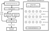 |
Fig. 1 Pictorial representation of the LRPayne workflow (left) and architecture of the artificial neural network used in LRPayne (right). |
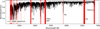 |
Fig. 2 Solar spectrum (black) with masked pixels indicated by vertical red lines. Important masked lines and data gap are described in text. |
2.4 Synthetic spectra
The synthetic stellar library was generated using 1D MARCS12 atmospheric models (Gustafsson et al. 2008) and the Turbospectrum synthesis code (Alvarez & Plez 1998; Plez 2012) within iSpec. The model atmospheres are 1D plane-parallel models under the local-thermodynamic equilibrium (LTE) approximations. We created the linelist used for the analysis by supplementing the atomic lines from the Gaia-ESO survey (GES) linelist with lines from Vienna Atomic Line Database (VALD).
We computed 70000 synthetic spectra with a total of 30 varying parameters: six physical parameters (Teff, logg, [Fe/H], vmic, vmac, and v sin i) and 24 atomic abundances (Li, C, N, O, Na, Al, Mg, Si, Ti, K, Ca, Mn, Cr, Ni, S, V, Sc, Ba, La, Eu, Y, Zn, Zr, and Cu). The physical parameter space was selected to ensure full coverage of FGK stars across all evolutionary stages. For this reason, the bounds for the effective temperature, Teff, were set between 4000 and 8000 K, with log g between 0.0 and 5.0 dex and metallicities between −2.5 and 0.5 dex. The values for these parameters were randomly drawn within these bounds, and we compared the Teff and log g values with a set of MIST stellar evolutionary tracks of FGK stars to include physically plausible combinations. We calculated the values of vmic and vmax for each star from the values of Teff, log g, and [Fe/H] using empirical relations (see Blanco-Cuaresma et al. (2014a). As the analysis was carried out on low-resolution spectra, we restricted v sin i to the range 2-20 km s−1, in steps of 2 km s−1. All abundance ratios [X/Fe] were randomly drawn from −0.5 to 0.5 dex, with solar abundances taken from Asplund et al. (2009). The parameter ranges are summarised in Table 1. Once the spectra were generated, they were degraded to the desired resolution of 5000 and resampled to match the wavelength grid of WEAVE-LR (four wavelength pixels per Å).
Parameter space used in this study.
2.5 Observed spectra
2.5.1 Data
The observed spectroscopic data were used for the astrophysical verification of the algorithm. As the algorithm was primarily designed to analyse low-resolution WEAVE data, it was important that the observed data had properties similar to those of WEAVE data. The resolution is straightforward to manage, as any higher-resolution spectra can be degraded to a resolution of choice. The biggest hurdle was to find data with full optical coverage comparable to WEAVE (3660 to 9590 Å). This requirement greatly narrowed the set of instruments from which data could be used. Therefore, instead of using this entire range, we conducted our analysis over 4200-6900 Å, a range covered by prominent instruments such as HARPS (Pepe et al. 2000), HARPS-N (Cosentino et al. 2012), FEROS (Kaufer et al. 1997), and NARVAL (Aurière 2003), which contain most of the usable key features in the optical spectrum. Using this range, we divided our verification sample into Gaia FGK benchmark stars and metal-poor stars taken from Bensby et al. (2014).
The Gaia FGK benchmark stars are a set of calibration stars defined in Heiter et al. (2015) and Hawkins et al. (2016) that cover a wide range of parameter space and have been analysed to minimise the dependence of stellar parameter estimations on spectroscopic and atmospheric models. Of the 34 stars, we included 23 stars in our analysis because they fell within our parameter space and possessed data with sufficient wavelength coverage. The stellar parameters for these stars in the literature were taken from Heiter et al. (2015) and Jofré et al. (2014). The observations were carried out using instruments such as HARPS, NARVAL, and ESPaDOnS (Manset & Donati 2003), with resolutions between 65 000 and 115 000 and S/N between 100 and 1000 per Å, and were downloaded from the Gaia FGK spectral library (Blanco-Cuaresma et al. 2014b)13. The available abundances for these stars are Mg, Si, Ca, Ti, Sc, V, Mn, Cr, Co, and Ni, and the values were obtained from Jofré et al. (2015) and Jofré et al. (2017).
To increase the verification sample and ensure good coverage of the entire parameter space (especially the metal-poor region), we also included stars from Bensby et al. (2014) (hereafter referred to as metal-poor stars). An advantage of this dataset is the availability of Na abundance, which is key to identifying first- and second-generation stars within clusters. All spectroscopic observations for these stars were carried out using the HARPS spectrograph and are available in the ESO archive. These spectra cover a wavelength range of 4200-6900 Å (with a gap of 30 Å at 5300 Å) and have a lower S/N than the benchmark stars, typically between 50 and 300 per Å. From Bensby et al. (2014), we obtained stellar parameters and abundances of O, Na, Mg, Al, Si, Ca, Ti, Cr, Fe, Ni, Zn, and Y.
2.5.2 Pre-processing
We obtained the spectra for different stars from three different instruments at different resolutions and wavelength coverages. To homogenise the entire sample to match the required specifications, we created a pre-processing pipeline. This pipeline relies heavily on functions defined within the iSpec tool14 (Blanco-Cuaresma et al. 2014a; Blanco-Cuaresma 2019). The pipeline proceeded as follows, with the corresponding iSpec functions indicated in parentheses:
We extracted the wavelength, flux, and spectral resolution from the fits header.
We restricted the spectral range to 4200-6900 Å, removing the rest.
We estimated the radial velocity using a cross-correlation method with the high-S/N solar spectrum as the template (see Blanco-Cuaresma et al. (2014a) for more details). After determining the velocity, we corrected the spectrum to the rest frame (determine_radial_velocity_with_mask and correct_velocit y).
When multiple radial velocity-corrected spectra existed for the same star and instrument, we merged them to improve the S/N of the resultant spectrum. For this, we simply took the median or the mean (for stars with only two spectra) of the flux at each wavelength point.
For continuum normalisation, we first divided each spectrum into ten segments of roughly 270 Å (except one segment due to a data gap). Within each segment, we estimated continuum points using a median and maximum filter, ensuring that strong absorption lines were excluded (wavelength ranges of several strong absorption lines, such as hydrogen Balmer lines, were provided). Using these points, we used multiple spline functions with degrees equal to one to model the continuum. The flux was divided by this continuum to obtain the normalised spectrum (fit_continuum, normalize _ spectrum ).
For several stars, the estimated continuum was slightly above the true continuum and was worse with a lower S/N spectrum. To remove this, we divided the entire spectrum by an offset estimated from the median flux of the continuum.
The co-added spectrum remained at high-resolution, so we degraded the resolution to R = 5000 via convolution with a Gaussian (convolve_spectrum).
We resampled the convolved spectrum using linear interpolation at four points per Å, producing spectra of approximately 10 799 pixels in length. This is in agreement with the low-resolution spectrum of the WEAVE survey.
These convolved spectra were used as the verification sample to test the reliability of the neural network’s performance on real observed spectra.
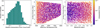 |
Fig. 3 Histogram of median interpolation errors from the ANN for 5000 synthetic models (left); correlation of interpolation errors with effective temperature and surface gravity of the synthetic models (middle); and correlation of interpolation error with metallicity and surface gravity (right) of the synthetic models. |
3 Results
3.1 Internal accuracy
To verify the performance of LRPayne, we used the same two tests employed by Ting et al. (2019). We generated an additional 5000 synthetic spectra for the two internal accuracy tests; these form the synthetic verification sample. These spectra were unseen by the neural network during its training. The first test examined the interpolation accuracy of the neural network by comparing a synthetic spectrum generated using Turbospectrum to the spectrum interpolated by the neural network for the same labels. The results for the 5000 synthetic validation sample are shown in Figure 3, where the first panel presents the median difference between the constructed and synthetic spectra, and the next two panels illustrate the interpolation accuracy across the parameter space. The neural network has an interpolation error of less than 1.3 × 10⁻³ for 90% of the sample, which translates to an error of less than 0.13%. The maximum interpolation error is 9.5 × 10⁻³ (less than 1%) for cool, metal-rich dwarfs. This trend is clearly evident in the second and third panels of Figure 3, where cooler, metal-rich stars exhibit relatively larger interpolation errors compared to the rest. This is expected as the spectra from these stars are rich in spectral lines, often blended together at low resolution, making it challenging to accurately interpolate. These results demonstrate the high interpolation accuracy of the neural network.
The second test examined how well the entire workflow could recover labels from synthetic models using χ2 minimisation. For this, we used the same synthetic validation sample at three different S/N: 1000, 100, and 20. We used iSpec’s Python function (add_noise) to degrade the S/N of the synthetic spectra. Although the added noise did not fully represent the real noise in an observed spectrum, it was sufficient to establish an upper limit on the accuracy of the tool to recover the labels at different S/N. Figure 4 shows the median differences between the input and recovered values for 30 parameters, obtained from fitting 5000 spectra. From the results at S/N =1000 and 100, we observe high accuracy for most parameters, except for Vsini, Li, and K. For Li and K, poor performance was expected due to the availability of only one or two lines, which are usually weak and blended. For Vsini, we observe a median discrepancy of approximately 2.5 kms−1. At S/N = 20, we observe a relatively larger discrepancy in Teff (~20 K) , Li (~0.22 dex), K (~0.1 dex), N (~0.28 dex), and Eu (−0.15 dex). Given the resolution, noisy spectra, and limited availability of suitable lines, such a decrease in accuracy is expected.
These two tests demonstrate the capabilities of LRPayne in handling model interpolation as well as in the extraction of stellar labels. The dispersions obtained in these tests represent a lower limit on the parameter uncertainties, which are expected to increase during the analysis of observed spectra because of effects such as incomplete physics in the synthetic regime, inaccurate continuum normalisation, and complex noise profiles.
3.2 Benchmark and metal-poor stars
Having obtained satisfactory results from the internal accuracy tests, we tested the ability of LRPayne to reliably recover stellar labels by fitting real observed spectra using an observed validation sample made up of 23 Gaia benchmark stars and 41 metal-poor stars. As mentioned above, spectral data for different stars originate from different instruments but have been pre-processed to match the instrumental characteristics of the low-resolution data from the WEAVE spectrograph. The results for stellar parameters and abundances are presented in Figures 5 and 6, respectively.
3.2.1 Parameters
In Figure 5, we compare the results obtained from LRPayne with those obtained from literature sources: Jofré et al. (2014) and Heiter et al. (2015) for benchmark stars and Bensby et al. (2014) for metal-poor stars. Heiter et al. (2015) derived the effective temperature using spectral energy distributions, interferometry, and distances, which in turn were used alongside luminosity and stellar masses derived through stellar evolutionary models to calculate the surface gravity of the star. Jofré et al. (2014) derived metallicities using the spectroscopic analysis of high-resolution spectroscopic data from instruments such as UVES, NARVAL, and HARPS (from the spectral library (Blanco-Cuaresma et al. 2014b)). They combined results from six different methods using the same atmospheric models and linelist. Bensby et al. (2014) used equivalent widths and the excitation equilibrium method for Fe I and Fe II lines to estimate stellar parameters using highresolution spectroscopy and then applied an non-local thermodynamic equilibrium (NLTE) correction to the derived parameters. The main reasons for selecting a study based on NLTE parameters to validate LTE-based LRPayne were: (1) it was one of the few studies to homogenously analyse a large sample of metalpoor stars using high-resolution spectroscopy, with instruments covering our desired wavelength range of 4200-6900 Å; (2) it estimated NLTE abundances of Na and Mg, two abundances of interest for Galactic archaeology studies of the outer halo using WEAVE-LR spectra; (3) the NLTE corrections applied to most stars were small (see Figure 6 in Bensby et al. (2014); (4) reduced spectra of stars observed with HARPS were readily available in the ESO archive; (5) additionally, it includes abundances such as O, Al, Zn, and Y, which are not available for benchmark stars, thereby aiding in validation of LRPayne for these elements. Before the comparison, we converted all parameters to the same solar scale, as Jofré et al. (2014) uses a solar iron abundance from Grevesse et al. (2007) [logA(Fe)⊙ = 7.45 dex], Bensby et al. (2014) uses a solar iron abundance of logA(Fe)⊙ = 7.58 dex, and our study is based on Asplund et al. (2009) with [logA(Fe)⊙ = 7.50 dex]. Therefore, we added 0.05 dex and subtracted 0.08 dex to the metallicities of the benchmark and metal-poor stars, respectively.
In Figures 5 and 6, taking into account the accuracy and uncertainties associated with parameter estimation at R = 5000 using the traditional method of excitation equilibrium of Fe lines, we define a range for each stellar label within which an estimate is considered satisfactory. For Teff, log(g), [Fe/H], and [X/Fe], this is set to ± 150 K, ± 0.3 dex, ± 0.3 dex and ± 0.3 dex, respectively (Re Fiorentin et al. 2007). We find a good agreement for most stars in our validation sample. We obtain a difference of 22±87 K, 0.19±0.23 dex, 0.01 ±0.17 dex, and −0.02±0.11 dex for Teff, log(g), [Fe/H], and [α∕Fe], respectively. Although there is overall good agreement in Teff, we observe a clear trend in the values of metal-poor stars. The trend between 5500 K and 6500 K can be attributed to the NLTE versus LTE difference, because, as explained in Bensby et al. (2014), even if the NLTE correction was negligible for stars with Teff < 5500 K, the scatter of correction values increases for hotter stars, consistent with the trend seen in Figure 5. Among these parameters, we find a large mean and standard deviation in log(g), due to two extreme outlier stars with ∆ log(g) ~ 1.0 dex. The two stars, HIP 22068 [6200 K, 4.18 dex, −1.34 dex] and HIP 60632 [6140 K, 4.07 dex, −1.67 dex], are both hot metal-poor dwarfs. We see a similar trend in other hot metal-poor dwarfs, such as HD 196892, HD 97320, and HD 84937, where log(g) is underestimated to a lesser extent (∆ log(g) ~ 0.40 dex). A major reason for the bias is the comparison of LTE results with NLTE values. In Figure 6 of Bensby et al. (2014), the change in log(g) from LTE to NLTE is between 0.1 and 0.3 dex for stars with [Fe/H] ≤ −1.0 dex. Three of the discrepant stars mentioned above are affected by this and fall into the satisfactory range when the NLTE effect is taken into account. In addition, the scarcity of good Fe II lines may contribute as these are key to an accurate log(g) determination. At these temperatures and metallicities, almost all of the Fe II lines are too weak for the neural network to fit accurately and therefore usually underestimate log(g). Even in [a/Fe], we see a trend with overestimation for [a/Fe]-poor stars and underestimation for [a/Fe]-rich stars. However, this is not significant due to uncertainties associated with the values in the literature (~0.1 dex). We note that our validation sample does not contain any metalpoor giants.; caution is advised when using LRPayne to analyse stars with surface gravities less than 2.5 and metallicities less than −1.3 dex.
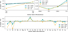 |
Fig. 4 Comparison of input labels with values recovered by LRPayne from fitting multiple synthetic spectra at different S/N (green: S/N = 20, red: S/N = 100 and black: S/N = 1000). Only 14 elements (O, Na, Al, Mg, Si, Ti, Ca, Mn, Cr, Ni, V, Sc, Ba, and Y) have been validated using observed data (See Section 3.2.2). For other elements, this result represents the upper limit of LRPayne sensitivity. |
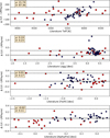 |
Fig. 5 Parameters inferred for Gaia FGK benchmark stars (red circles) and metal-poor stars (blue plus signs) using LRPayne compared with literature values. The solid black line represents zero difference; the two dashed black lines represent a range within which the accuracy of LRPayne is comparable to traditional methods of analysis. Literature parameters are from Jofré et al. (2014) and Heiter et al. (2015) for benchmark stars and Bensby et al. (2014) for metal-poor stars. The mean and 1σ of the distribution appear in the top left corner of each panel. |
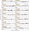 |
Fig. 6 Comparison of abundances for 14 elements obtained from LRPayne and the literature. The red circles represent benchmark stars and dark blue plus signs represent metal-poor stars. The solid black line indicates zero difference, while the dashed black lines represent ∆ = ±0.3 dex. |
3.2.2 Abundances
Even though LRPayne has been trained to simultaneously fit 24 elemental abundances, we are able to reliably verify its performance on actual data for only 14 of them. This is because few studies provide homogeneous analyses across various star types (in terms of coverage of the parameter space) and determine abundances for elements such as Li, Na, α-, Fe-peak, s-process and r-process elements. Therefore, we limited our validation to the abundances present in Bensby et al. (2014), Jofré et al. (2015), and Jofré et al. (2017). In Figure 6, we compare the abundances obtained from LRPayne with those from the literature.
3.2.3 α elements
Among the α elements, we verify five abundances: O, Mg, Si, Ti, and Ca. We note that although Ti is not an α element, it is included here as it behaves similarly to an α element. Oxygen is generally difficult to analyse in the optical spectrum as a result of the absence of strong CO and OH molecular bands; therefore, when available, most studies use the infrared spectrum. Within our desired wavelength range, the two forbidden oxygen lines at 6300 and 6363 Å are most commonly used to derive the oxygen abundance. However, they face two issues. Firstly, the two lines are in regions affected by telluric absorption, so depending on the radial velocity of the star, the lines can easily become blended with telluric lines. Secondly, both lines are generally weak, with the line at 6363 Å falling below the detection limit in most stars (depending on stellar parameters) even at very high S/N. A third issue is the NLTE correction (roughly 0.1 dex) applied to these abundances in Bensby et al. (2014). Despite these limitations, LRPayne recovers the oxygen abundance for 18 of the 31 stars, or about 60% of the sample, after taking into account the uncertainties in the literature values, which are on average 0.15 dex. When the NLTE correction is taken into account, 20 stars fall within the satisfactory range. Although the majority of the stars are well fitted, the remaining 13 stars are highly discrepant, which leads to a large mean offset of 0.49 dex. Only a portion of the large discrepancy can be explained by a combination of uncertainties in the literature values and the NLTE corrections applied by Bensby et al. (2014); the remainder is attributed to the difficulties associated with measuring oxygen abundance in the optical spectrum.
Among the other four α elements, LRPayne performs the best on [Si/Fe], with a mean offset of 0.01 dex. It also shows better accuracy on the benchmark stars compared to the metal-poor ones. However, when considering the applicable uncertainties, all stars except two fall within ± 0.3 dex of the literature values. For [Mg/Fe], the mean offset is larger than for [Si/Fe] at 0.09 dex, but with an average uncertainty of 0.09 dex on the literature values, the results are in good agreement. For [Ti/Fe] and [Ca/Fe], the mean offsets are larger than [Mg/Fe], at 0.15 and 0.12 dex, respectively. Most stars in [Ti/Fe] agree with the literature when uncertainties are taken into account, except for three metal-poor stars, which are discrepant by more than 0.5 dex and contribute to increase in mean offset. The [Ca/Fe] abundance follows the same trend as that of [Ti/Fe], with most stars in good agreement, except for three. These three stars, HIP 22068, HIP 60631, and HD 104006, are the same for both abundances, with two being hot metal-poor dwarf stars. The discrepancy in the estimation of their log(g) contributes to the discrepancies in Ti and Ca.
3.2.4 Odd-Z element
Within the odd-Z elements, we verify Na and Al using abundances taken from Bensby et al. (2014). We corrected all sodium abundances from Bensby et al. (2014) for NLTE effects; however, because these corrections are negligible, LRPayne reliably recovers the abundances for all but one star. The mean offset (μ) for [Na/Fe] is −0.07 dex, which is close to the average uncertainty of 0.05 dex in the literature values. Therefore, there is good agreement between the two; however, as Al has very few suitable lines for abundance analysis that are also weak and blended, it is a challenging element to measure accurately. We find a similar case with LRPayne, as it struggles to accurately fit [Al/Fe] in many stars. Approximately 19 stars, or about 48%, are within ±0.3 dex of the literature value; roughly 25% of the stars have a discrepancy larger than 0.5 dex. Examining the discrepant stars reveals a direct correlation between the discrepancy and stellar metallicity, i.e. the more metal-poor a star is, the larger the discrepancy. This trend is expected because lower metallicity produces weaker spectral lines and, for an element such as Al, the few suitable lines become considerably weak. We also see a trend between the accuracy of LRPayne on [Al/Fe] and the log(g) of the star, with higher log(g) values, i.e. dwarf stars, showing poor accuracy.
3.2.5 Fe-peak elements
Among Fe-peak elements, we investigated five abundances: Sc, V, Cr, Mn, and Ni. Among these elements, Bensby et al. (2014) provides only Cr and Ni for the metal-poor stars; therefore, we considered Sc, V, and Mn for the benchmark stars. The overall accuracy of LRPayne on Fe-peak elements is good, except for Mn. The other four abundances show excellent agreement with the literature values when uncertainties are considered. Only two stars are discrepant in [Cr/Fe] and [Ni/Fe]; these are the same hot metal-poor dwarf stars that show discrepancies in log(g) and the α elements. The mean offsets of [Cr/Fe] and [Ni/Fe] are 0.07 and 0.04 dex, respectively. These offsets are smaller than the average uncertainties associated with the literature values. For [V/Fe] and [Sc/Fe], all stars fall within ± 0.3 dex of the literature value, and considering uncertainties, most of the values are easily within 1 σ of the literature values. However, for [Mn/Fe], LRPayne reliably recovers the abundance only for stars with [Mn/Fe] > -0.25 dex. The reliability decreases significantly for [Mn/Fe] < -0.25 dex, with only three of the nine stars within ±0.3 dex of the literature values. We also find that the stars with high discrepancies are all metal-rich giants, whereas stars within ±0.3 dex of the literature values are all dwarf stars. The most likely reason for the behaviour of LRPayne is the saturation of the Mn lines, which is more likely in giant stars than dwarfs. Such saturation effects remove any correlation between the elemental abundance and the spectral line strength, making it difficult for the neural network to reproduce the underlying relationship.
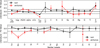 |
Fig. 7 Uncertainties in stellar labels for the Sun (black) and Arcturus (red). Values for Arcturus are missing where literature data are unavailable. The uncertainties shown are from LRPayne, with literature errors assumed to be zero to highlight fitting errors. |
3.2.6 Heavy elements
Among the heavy elements, we verify two s-process elements, Ba and Y, using the metal-poor stars. Although Figure 6 shows an apparent offset for [Ba/Fe] and a large scatter for [Y/Fe], more than 70% of the stars fall within ±0.3 dex of the literature value when uncertainties are considered. This is due to the large average uncertainties of 0.10 dex for [Ba/Fe] and 0.16 dex for [Y/Fe].
3.2.7 Uncertainties
Within the LRPayne workflow, there are two sources of uncertainties associated with parameter estimation. One is the fitting error of the χ2 minimisation process, while the other originates from the variation in the trained ANN models due to random initialisation during each training run.
To probe both sources, we employed an Markov chain Monte Carlo (MCMC)-like methodology. We trained ten different ANN models using different shuffling of the training set while keeping all the hyper-parameters the same. For each of the ten models, a star passes through the entire workflow 2000 times, with only the initial guess for the χ2 minimisation process being varied. We repeated this procedure for all ten models, resulting in a total of 20 000 fitting procedures performed per star. This generated a posterior distribution for each of the parameters, from which we measured the uncertainties, with 1σ corresponding to the 16th and 86th percentile of the distribution. This method accounts for both sources of uncertainty: the fitting error is considered by repeating the χ2 minimisation 2000 times, and variations in trained models are considered by fitting the same star with ten different models. The uncertainties were estimated for ten stars that cover a wide range of the parameter space. The limited sample size is due to the extensive computation time required for the uncertainty analysis of each star. Figure 7 shows the uncertainties associated with the stellar labels for the Sun (S/N ~ 500) and Arcturus (S/N ~ 500). For most stellar labels, the uncertainties are reasonable, and the errors on stellar parameters are acceptable for both stars. The largest uncertainties are obtained for elements such as Li, O, Al, K, S, Eu, and Zn, which are generally difficult to estimate in low-resolution spectra. For the remaining elements, the average uncertainties in abundances are approximately 0.13 dex for Sun and 0.21 dex for Arcturus. An interesting trend is that, for stellar parameters and abundances that are well fitted by LRPayne, the uncertainties associated with Arcturus are larger than those associated with the Sun. This could be a result of giant stars having more spectral features than dwarf stars, leading to an increase in interpolation error. Table 2 summarises the uncertainties for different stellar labels, depending on the type of star.
3.2.8 Dependency on S/N
As our primary objective is to use LRPayne to analyse low-resolution data of a spectroscopic survey mission, it is important to understand how the quality of the spectrum affects the reliability of LRPayne. Generally, as surveys try to find a balance between number of observed stars and quality of those observations, the data very rarely tends to have a high S/N (>100 per Å). To test this, we use LRPayne to fit three solar spectra with different amounts of noise added to them. The S/N of the three spectra is 10, 30 and 100. The results of the fitting is shown in Figure 8. From the figure, it is evident that the reliability of LRPayne upon fitting a 30 S/N spectrum is almost the same as fitting a 100 SNR spectrum. Only at very low S/N of 10, we see the results deviating more from the literature values. This result shows that LRPayne is highly capable of handling spectral data with lower S/N.
4 Summary
In this paper, we present LRPayne, a neural network-based algorithm specifically designed for the analysis of low-resolution optical spectra from large-scale galactic surveys. Our algorithm is an adaptation of The Payne and employs a fully connected artificial neural network with three hidden layers. The training set comprised 70 000 synthetic stellar spectra generated using the Turbospectrum code within iSpec, 1D MARCS atmosphere models, and a modified (GES + VALD) linelist. The algorithm analyses spectra degraded to R = 5000 over 4200-6900 Å, making it ideal for surveys such as WEAVE. Our key findings are summarised below:
Technical performance: Internal accuracy tests demonstrate that LRPayne achieves excellent interpolation accuracy, with median errors of less than 0.13% for 90% of the synthetic validation sample. The algorithm successfully recovers input stellar parameters and abundances from synthetic spectra, even at S/N=20, though with expected degradation in accuracy for challenging elements such as Li, K, and N;
Stellar parameters: Validation on 64 real stars (23 Gaia FGK benchmark stars and 41 metal-poor stars) reveals robust performance for the fundamental stellar parameters. We obtain mean differences of 22 ± 87 K in effective temperature, 0.19 ± 0.23 dex in surface gravity, and 0.01 ± 0.17 dex in metallicity relative to literature values. The algorithm shows a particular strength in determining effective temperatures and metallicities across a wide range of stellar types;
Chemical abundances: LRPayne demonstrates reliable abundance determination for multiple elements across different nucleosynthetic groups. Elements such as Na, Mg, Si, and most Fe-peak elements (Cr, Ni, V, and Sc) show typical accuracies of 0.1-0.2 dex. The algorithm successfully determines abundances for α-elements (Mg, Si, Ti, and Ca), Fe-peak elements (Sc, V, Cr, and Ni), and heavy elements (Ba and Y), providing crucial information for Galactic archaeology studies;
Challenges and limitations: We identify specific challenges in the analysis of certain stellar types and elements. The determination of oxygen abundance remains difficult because of the weakness of optical oxygen lines and telluric contamination. Manganese abundances exhibit systematic biases in metal-rich giants, likely caused by line saturation effects. Aluminium abundances are challenging in metalpoor stars and dwarfs due to weak spectral features. Surface gravity determination for hot metal-poor dwarfs shows a systematic underestimation, partly attributable to LTE-NLTE differences and the weakness of FeII lines in this parameter regime. Another important challenge is the substantial adverse effect of the synthetic gap on the performance of the neural network. If not accounted for, this gap can easily derail the analysis, leading to incorrect results and conclusions. Masking the wavelength pixels provides a simple correction, but future sophisticated methods to handle the synthetic gap may minimise information loss. Finally, although LRPayne performs well on the verification sample, the sample size remains small. A more comprehensive analysis is needed to fully characterise the behaviour of LRPayne, but this will only be possible with the commencement of surveys such as WEAVE and 4MOST;
Signal-to-noise performance: LRPayne maintains robust performance down to S/N ~ 30, with only modest degradation compared to high-S/N spectra. This capability is crucial for survey applications, where achieving uniformly high S/N across all targets is impractical;
Immediate application: The algorithm demonstrates particular efficacy in determining abundances of key elements such as Na and Mg, which are crucial tracers for identifying first-generation (1G) and second-generation (2G) stellar populations within Galactic globular clusters. We plan to use LRPayne to analyse WEAVE low-resolution data to identify and characterise these populations, and thereby improve our understanding of their formation and evolution within globular clusters.
Uncertainties in stellar labels for stars with different stellar parameters.
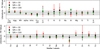 |
Fig. 8 Comparison of LRPayne fitted values with literature values for solar spectra at three different S/N(S/N = 10: red circles; S/N = 30: black squares; and S/N = 100: green diamonds). LRPayne uncertainties are shown, assuming zero literature errors assumed to highlight fitting errors. |
References
- Abadi, M., Agarwal, A., Barham, P., et al. 2015, TensorFlow: Large-Scale Machine Learning on Heterogeneous Systems, software available from https://tensorflow.org [Google Scholar]
- Alvarez, R., & Plez, B. 1998, A&A, 330, 1109 [NASA ADS] [Google Scholar]
- Asplund, M., Grevesse, N., Sauval, A. J., & Scott, P. 2009, ARA&A, 47, 481 [CrossRef] [Google Scholar]
- Aurière, M. 2003, in EAS Publications Series, eds. J. Arnaud, & N. Meunier, 9, 105 [Google Scholar]
- Bensby, T., Feltzing, S., & Oey, M. S. 2014, A&A, 562, A71 [NASA ADS] [CrossRef] [EDP Sciences] [Google Scholar]
- Blanco-Cuaresma, S. 2019, MNRAS, 486, 2075 [Google Scholar]
- Blanco-Cuaresma, S., Soubiran, C., Heiter, U., & Jofré, P. 2014a, A&A, 569, A111 [CrossRef] [EDP Sciences] [Google Scholar]
- Blanco-Cuaresma, S., Soubiran, C., Jofré, P., & Heiter, U. 2014b, A&A, 566, A98 [NASA ADS] [CrossRef] [EDP Sciences] [Google Scholar]
- Cosentino, R., Lovis, C., Pepe, F., et al. 2012, SPIE Conf. Ser., 8446, 84461V [Google Scholar]
- Cui, X.-Q., Zhao, Y.-H., Chu, Y.-Q., et al. 2012, Res. Astron. Astrophys., 12, 1197 [Google Scholar]
- Dalton, G., Trager, S. C., Abrams, D. C., Carter, D., & Bonifacio, P. E. A. 2012, SPIE Conf. Ser., 8446, 84460P [NASA ADS] [Google Scholar]
- de Jong, R. S., Agertz, O., Berbel, A. A., et al. 2019, The Messenger, 175, 3 [NASA ADS] [Google Scholar]
- De Silva, G. M., Freeman, K. C., Bland-Hawthorn, J., et al. 2015, MNRAS, 449, 2604 [NASA ADS] [CrossRef] [Google Scholar]
- DESI Collaboration (Aghamousa, A., et al.) 2016, arXiv e-prints [arXiv:1611.00036] [Google Scholar]
- Euclid Collaboration (Jahnke, K., et al.) 2025, A&A, 697, A3 [Google Scholar]
- Fabbro, S., Venn, K. A., O’Briain, T., et al. 2018, MNRAS, 475, 2978 [Google Scholar]
- Gaia Collaboration (Vallenari, A., et al.) 2023, A&A, 674, A1 [NASA ADS] [CrossRef] [EDP Sciences] [Google Scholar]
- Gilmore, G., Randich, S., Asplund, M., et al. 2012, The Messenger, 147, 25 [NASA ADS] [Google Scholar]
- Grevesse, N., Asplund, M., & Sauval, A. J. 2007, Space Sci. Rev., 130, 105 [Google Scholar]
- Gustafsson, B., Edvardsson, B., Eriksson, K., et al. 2008, A&A, 486, 951 [NASA ADS] [CrossRef] [EDP Sciences] [Google Scholar]
- Hawkins, K., Jofré, P., Heiter, U., et al. 2016, A&A, 592, A70 [NASA ADS] [CrossRef] [EDP Sciences] [Google Scholar]
- He, K., Zhang, X., Ren, S., & Sun, J. 2015, arXiv e-prints [arXiv:1502.01852] [Google Scholar]
- Heiter, U., Jofré, P., Gustafsson, B., et al. 2015, A&A, 582, A49 [NASA ADS] [CrossRef] [EDP Sciences] [Google Scholar]
- Jin, S., Trager, S. C., Dalton, G. B., Aguerri, J. A. L., & Drew, J. E. e. a. 2024, MNRAS, 530, 2688 [NASA ADS] [CrossRef] [Google Scholar]
- Jofré, P., Heiter, U., Soubiran, C., et al. 2014, A&A, 564, A133 [NASA ADS] [CrossRef] [EDP Sciences] [Google Scholar]
- Jofré, P., Heiter, U., Soubiran, C., et al. 2015, A&A, 582, A81 [Google Scholar]
- Jofré, P., Heiter, U., Worley, C. C., et al. 2017, A&A, 601, A38 [Google Scholar]
- Kaufer, A., Wolf, B., Andersen, J., & Pasquini, L. 1997, The Messenger, 89, 1 [NASA ADS] [Google Scholar]
- Kingma, D. P., & Ba, J. 2014, arXiv e-prints [arXiv:1412.6980] [Google Scholar]
- Majewski, S. R., Schiavon, R. P., Frinchaboy, P. M., & Allende Prieto, C. E. A. 2017, AJ, 154, 94 [NASA ADS] [CrossRef] [Google Scholar]
- Manset, N., & Donati, J.-F. 2003, SPIE Conf. Ser., 4843, 425 [Google Scholar]
- Montegriffo, P., De Angeli, F., Andrae, R., et al. 2023, A&A, 674, A3 [NASA ADS] [CrossRef] [EDP Sciences] [Google Scholar]
- Ness, M., Hogg, D. W., Rix, H. W., Ho, A. Y. Q., & Zasowski, G. 2015, ApJ, 808, 16 [NASA ADS] [CrossRef] [Google Scholar]
- Pepe, F., Mayor, M., Delabre, B., et al. 2000, SPIE Conf. Ser., 4008, 582 [NASA ADS] [Google Scholar]
- Plez, B. 2012, Turbospectrum: Code for spectral synthesis, Astrophysics Source Code Library [record ascl:1205.004] [Google Scholar]
- Re Fiorentin, P., Bailer-Jones, C. A. L., Lee, Y. S., et al. 2007, A&A, 467, 1373 [NASA ADS] [CrossRef] [EDP Sciences] [Google Scholar]
- Steinmetz, M., Zwitter, T., Siebert, A., et al. 2006, AJ, 132, 1645 [Google Scholar]
- Ting, Y.-S., Conroy, C., Rix, H.-W., & Cargile, P. 2019, ApJ, 879, 69 [Google Scholar]
WHT Enhanced Area Velocity Explore.
4-metre Multi-Object Spectroscopic Telescope.
Dark Energy Spectroscopic Instrument.
Apache Point Observatory Galactic Evolution Experiment.
The Radial Velocity Experiment.
Large Sky Area Multi-Object Fiber Spectroscopic Telescope.
GALactic Archaeology with HERMES.
Near Infrared Spectrometer and Photometer.
Radial Velocity Spectrometer.
Model Atmospheres with a Radiative and Convective Scheme.
iSpec is a software written in Python to perform spectroscopic analysis such as radial velocity estimation, determination of stellar parameters, and abundance estimation.
All Tables
All Figures
|
Fig. 1 Pictorial representation of the LRPayne workflow (left) and architecture of the artificial neural network used in LRPayne (right). |
| In the text | |
|
Fig. 2 Solar spectrum (black) with masked pixels indicated by vertical red lines. Important masked lines and data gap are described in text. |
| In the text | |
|
Fig. 3 Histogram of median interpolation errors from the ANN for 5000 synthetic models (left); correlation of interpolation errors with effective temperature and surface gravity of the synthetic models (middle); and correlation of interpolation error with metallicity and surface gravity (right) of the synthetic models. |
| In the text | |
|
Fig. 4 Comparison of input labels with values recovered by LRPayne from fitting multiple synthetic spectra at different S/N (green: S/N = 20, red: S/N = 100 and black: S/N = 1000). Only 14 elements (O, Na, Al, Mg, Si, Ti, Ca, Mn, Cr, Ni, V, Sc, Ba, and Y) have been validated using observed data (See Section 3.2.2). For other elements, this result represents the upper limit of LRPayne sensitivity. |
| In the text | |
|
Fig. 5 Parameters inferred for Gaia FGK benchmark stars (red circles) and metal-poor stars (blue plus signs) using LRPayne compared with literature values. The solid black line represents zero difference; the two dashed black lines represent a range within which the accuracy of LRPayne is comparable to traditional methods of analysis. Literature parameters are from Jofré et al. (2014) and Heiter et al. (2015) for benchmark stars and Bensby et al. (2014) for metal-poor stars. The mean and 1σ of the distribution appear in the top left corner of each panel. |
| In the text | |
|
Fig. 6 Comparison of abundances for 14 elements obtained from LRPayne and the literature. The red circles represent benchmark stars and dark blue plus signs represent metal-poor stars. The solid black line indicates zero difference, while the dashed black lines represent ∆ = ±0.3 dex. |
| In the text | |
|
Fig. 7 Uncertainties in stellar labels for the Sun (black) and Arcturus (red). Values for Arcturus are missing where literature data are unavailable. The uncertainties shown are from LRPayne, with literature errors assumed to be zero to highlight fitting errors. |
| In the text | |
|
Fig. 8 Comparison of LRPayne fitted values with literature values for solar spectra at three different S/N(S/N = 10: red circles; S/N = 30: black squares; and S/N = 100: green diamonds). LRPayne uncertainties are shown, assuming zero literature errors assumed to highlight fitting errors. |
| In the text | |
Current usage metrics show cumulative count of Article Views (full-text article views including HTML views, PDF and ePub downloads, according to the available data) and Abstracts Views on Vision4Press platform.
Data correspond to usage on the plateform after 2015. The current usage metrics is available 48-96 hours after online publication and is updated daily on week days.
Initial download of the metrics may take a while.