| Issue |
A&A
Volume 706, February 2026
|
|
|---|---|---|
| Article Number | A337 | |
| Number of page(s) | 9 | |
| Section | Cosmology (including clusters of galaxies) | |
| DOI | https://doi.org/10.1051/0004-6361/202556703 | |
| Published online | 20 February 2026 | |
The redshift and X-ray photon index evolutionary LX-LUV relations of quasars
1
China Institute of Atomic Energy Beijing 102413, China
2
Jinping Deep Underground Frontier Science and Dark Matter Key Laboratory of Sichuan Province Liangshan 615000, China
3
School of Nuclear Science and Technology, University of Chinese Academy of Sciences Beijing 101408, China
★ Corresponding author: This email address is being protected from spambots. You need JavaScript enabled to view it.
; This email address is being protected from spambots. You need JavaScript enabled to view it.
Received:
1
August
2025
Accepted:
9
January
2026
Abstract
The LX-LUV relation serves as a cornerstone for extending the Hubble diagram to higher redshift by utilizing quasars as standard candles. However, the constancy of the LX-LUV relation has been embroiled in controversy recently. In this work, we discuss the possible physical origins of evolution in the luminosity relation and provide explicit forms for the redshift and ΓX dependences. By calibrating quasar distances with the baryon acoustic oscillation measurements from the Dark Energy Spectroscopic Instrument Data Release 2 in combination with the cosmic microwave background measurements from Planck, the parameters in different luminosity relations are constrained with a clean quasar sample. Our analysis indicates strongly that the LX-LUV relation varies simultaneously with redshift and ΓX, and this conclusion is robust under the cosmological model assumptions. Furthermore, the dependence on redshift and ΓX implies that the LX-LUV relation is influenced by the properties of accreting supermassive black holes.
Key words: quasars: emission lines / cosmological parameters
© The Authors 2026
 Open Access article, published by EDP Sciences, under the terms of the Creative Commons Attribution License (https://creativecommons.org/licenses/by/4.0), which permits unrestricted use, distribution, and reproduction in any medium, provided the original work is properly cited.
This article is published in open access under the Subscribe to Open model. This email address is being protected from spambots. You need JavaScript enabled to view it. to support open access publication.
1. Introduction
The motion information of the Universe is encoded in the distance-redshift relation. To understand the evolutionary history of the Universe and the nature of dark energy, it is essential to continuously improve the measurement accuracy of cosmological distance and extend the Hubble diagram to higher redshifts (Riess et al. 1996; Perlmutter et al. 1997; Riess et al. 1998; Schmidt et al. 1998; Perlmutter et al. 1999; Timmes et al. 2003; Jha et al. 2007; Hicken et al. 2009; Kelly et al. 2010; Sullivan et al. 2010; Bravo et al. 2010; Suzuki et al. 2012; Johansson et al. 2013; Childress et al. 2013; Rigault et al. 2015, 2020; Kim et al. 2018; Roman et al. 2018; Jones et al. 2018; Risaliti & Lusso 2019; Rose et al. 2019; Riess et al. 2019; Barkhudaryan et al. 2019; Aghanim et al. 2020; Kang et al. 2020; Rose et al. 2020; Lee et al. 2020; Lusso et al. 2020; Murakami et al. 2021; Li & Li 2021; Riess et al. 2022; Hagstotz et al. 2022; Wu et al. 2022; Liu et al. 2023; Signorini et al. 2024; Trefoloni et al. 2024; Freedman et al. 2025). Quasars are extremely luminous energy sources in the Universe. They can be observed up to a redshift of ∼7.5 (Banados et al. 2018), corresponding to a time when the Universe was no more than 700 million years old. So it is quite natural to consider that if quasars can serve as distance indicators, they could provide insights into the expansion history of the Universe over the past more than 10 billion years.
Quasars, historically regarded as one of the ‘four great discoveries’ in astronomy in the 1960s, have been extensively studied over the past half century. It is now known that quasars, as a type of active galactic nucleus (AGN), release tremendous energy originating from the accretion of surrounding matter by the supermassive black holes (SMBHs) in the centres of galaxies. The intrinsic luminosities of quasars span multiple orders of magnitude, which precludes using them as traditional standard candles for distance calibration in the same way as type Ia supernovae (SNe Ia). Nonetheless, there exists a well-established non-linear correlation between the X-ray (at 2 keV) and ultraviolet (UV, at 2500 Å) emission; for example,  (Tananbaum et al. 1979; Risaliti & Lusso 2015, 2017; Lusso & Risaliti 2017; Risaliti & Lusso 2019; Lusso et al. 2019; Salvestrini et al. 2019; Lusso et al. 2020; Bisogni et al. 2021; Signorini et al. 2024; Trefoloni et al. 2024; Lusso et al. 2025). The non-linearity of the LX-LUV relation links the luminosity distance (dL) to the observed X-ray and UV fluxes (FX and FUV) via the relation between luminosities and fluxes, LUV(X) = 4πdL2FUV(X), enabling the inference of quasar distances from flux measurements and thereby enabling cosmological distance calibration. According to the widely accepted disc-corona model (Haardt & Maraschi 1993), the X-ray emission primarily originates from a hot relativistic electron plasma (the so-called corona) surrounding the accretion disc through inverse Compton scattering processes on the seed UV photons. The LX-LUV relation indicates the existence of a universal mechanism governing the energy transfer from the accretion disc to the hot corona. However, the underlying physics remains poorly understood.
The constancy of the LX-LUV relation is of vital importance for distance calibration and cosmological parameter constraints. However, the energy transfer and radiation mechanisms in quasars remain not fully understood. Thus, existing theories fail to provide a satisfactory explanation for the LX-LUV relation. They are also unable to demonstrate its universality across all the quasars. Moreover, some studies have suggested that the relation exhibits redshift dependence and proposed several possible evolutionary forms in the cosmological fits (Li et al. 2022; Wang et al. 2022, 2024; Li et al. 2025; Wu et al. 2025), which led to controversy over its constancy. Actually, the parameter γ in the LX-LUV relation obtained in the model-independent method and those obtained assuming various cosmological models show a discrepancy, which can be interpreted in two ways: a redshift evolution of the LX-LUV relation, or a shortcoming of the mainstream cosmological model (or its minimal variations). We decided to follow the first path, as some studies have suggested that the relation exhibits redshift dependence.
In principle, the energy transferred from the accretion disc to the corona most likely depends on the SMBH mass and accretion rate (Lusso & Risaliti 2017), so the LX-LUV relation may also be related to the properties of accreting SMBHs. If the SMBH mass or accretion rate exhibits a statistically significant redshift evolution, the LX-LUV relation is also likely to show redshift evolution. Furthermore, the coronal X-ray emission can be simply characterized by a power-law spectrum with a photon index (ΓX), such that the photon number is N(E)∝E−ΓX. The photon index, ΓX, is negatively correlated with the temperature of the Comptonizing electrons and the optical depth of the X-ray emitting plasma (Rybicki & Lightman 1979; Ricci et al. 2018). In addition, many studies have identified a correlation between ΓX and the Eddington ratio λEdd = Lbol/LEdd, where Lbol is the bolometric luminosity and LEdd is the Eddington luminosity (Kelly et al. 2008; Shemmer et al. 2008; Risaliti et al. 2009; Brightman et al. 2013; Gu & Cao 2009; Fausnaugh et al. 2016; Connolly et al. 2016). Since LEdd is proportional to the SMBH mass, some degree of correlation between ΓX and SMBH mass is also expected (Risaliti et al. 2009). Hence, the influence of SMBH properties on the emissions would be partially encoded in ΓX. If the LX-LUV relation indeed depends on SMBH properties, its parameters should correlate with ΓX. In principle, if the ΓX distribution of a quasar sample were perfectly unbiased and symmetric about its median, there would be no bias introduced into the cosmological analysis. Nevertheless, incorporating the ΓX dependence can further reduce the data dispersion, and thus enable more precise cosmological inferences. Moreover, for samples with a biased ΓX distribution, it is not necessary to filter the data carefully to maintain unbiasedness. Instead, a ΓX-dependent luminosity relation can be directly used to analyse the sample. Consequently, investigating the ΓX dependence also remains meaningful.
In recent years, with the continual improvement of astronomical observation accuracy and the rapid accumulation of data, the cosmic distance-redshift relation has been tightly constrained by mutiple probes, including SNe Ia, baryon acoustic oscillations (BAOs), cosmic microwave background (CMB), and so on (Aghanim et al. 2020; Riess et al. 2019, 2022; Scolnic et al. 2022; Riess et al. 2024; Breuval et al. 2024; Adame et al. 2025; Abdul Karim et al. 2025). In particular, the latest BAO measurements from the Dark Energy Spectroscopic Instrument (DESI) Data Release 2 (DR2) provide stringent constraints at high redshift. Consequently, the luminosity distance of quasars could be precisely determined based on the measured quasar redshifts and the well-constrained luminosity distance-redshift relation, enabling a more robust test of potential evolution in the LX-LUV relation. In this paper, the possible physical origins of the redshift and ΓX dependences of the LX-LUV relation are discussed at first. Then we propose several promising evolutionary models and constrain their parameters using a clean quasar sample, with quasar distances calibrated by the BAO measurements from the DESI DR2 in combination with CMB and SNe Ia datasets (Abdul Karim et al. 2025).
2. The method
From the perspective of the energy sources of quasars, whether the energy is transferred from infalling material to the accretion disc or from the disc to the corona, the process most likely depends on the SMBH mass (MBH) and accretion rate (Ṁ). Consequently, the UV and X-ray luminosities of quasars should be related to MBH and Ṁ. Assuming that the UV and X-ray emissions can be simply characterized by a power-law spectrum with a photon indices ΓUV and ΓX, respectively, the luminosities take the form
 (1)
(1)
where LUV and LX are the rest-frame monochromatic luminosities at 2500 Å and 2 keV, respectively. Here, CUV(X) is a constant, and the dependence on the SMBH properties is encapsulated in the function fUV(X) (MBH,Ṁ).
Although the exact form of fUV(X) is unknown, there are two compelling reasons to expect its evolution with time or redshift. First, from the physical evolution of accreting SMBHs: as the SMBH accumulates matter through accretion, the available gas is depleted, leading to evolution in MBH and Ṁ over cosmic time. Second, from the observational perspective: quasar samples at different redshifts are heterogeneous. Figure 1 illustrates the UV and X-ray monochromatic luminosities of quasars in different redshift intervals. Our analysis utilizes a sample of 2421 quasars spanning a redshift range of 0.009 < z < 7.52, with objects likely contaminated by dust reddening, host-galaxy emission, X-ray absorption, or affected by the Eddington bias filtered through a series of selection criteria (Lusso et al. 2020). The UV and X-ray monochromatic luminosities were estimated from measured fluxes assuming the cosmological constant Λ-cold dark matter (ΛCDM) cosmology with the Hubble constant H0 = 70 km s−1 Mpc−1 and the fractional energy density in matter ΩM = 0.3. It is evident from Figure 1 that the higher redshift samples tend to include more luminous quasars. This is a natural selection effect in observations, since quasars with lower luminosities at high redshift are not detectable at such distances. Nevertheless, the SMBH properties corresponding to low and high luminosity quasars may differ, implying that fUV(X) should be redshift-dependent.
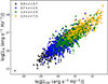 |
Fig. 1. UV and X-ray monochromatic luminosities of quasars in different redshift intervals. The luminosities were obtained from the measured fluxes assuming a standard ΛCDM cosmological model with H0 = 70 km s−1 Mpc−1 and ΩM = 0.3. |
To infer the possible redshift dependence of fUV(X), we examined the relation between log LUV(X) and log(1 + z) (Figure 2). Within the redshift range with adequate statistics, log LUV(X) increases approximately linearly with log(1 + z), suggesting that fUV(X) can be expressed as a power of (1 + z), i.e., fUV(X) = (1 + z)kUV(X). Substituting this into Equation (1), the relation between log LUV and log LX can be derived:
 (2)
(2)
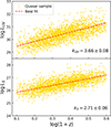 |
Fig. 2. UV (the upper panel) and X-ray (the lower panel) monochromatic luminosities (in units of erg s−1 Hz−1) of quasars varying with redshifts. The luminosities were obtained from the measured fluxes assuming a standard ΛCDM cosmological model with H0 = 70 km s−1 Mpc−1 and ΩM = 0.3. The log LUV(X) approximately linearly increases with log(1 + z) within the range of redshifts where the statistical quantity of sample is sufficient. The dashed red lines are the optimal linear fits, and kUV(X) are the corresponding slopes. |
where γ, β, and α depend on ΓX,
 (3)
(3)
 (4)
(4)
 (5)
(5)
If the redshift and ΓX dependences are neglected (i.e. α ≡ 0 and γ, β are constant), Equation (2) reduces to the standard LX-LUV relation.
Using the relation between luminosity and flux, Equation (2) can be transformed into a relation between observable fluxes,
 (6)
(6)
where
 (7)
(7)
The luminosity distance can be predicted from a cosmological model as
 (8)
(8)
where c is the speed of light, H0 is the Hubble constant representing the current expansion rate of the Universe, and E(z) denotes the dimensionless Hubble parameter encapsulating the cosmological evolution. For a spatially flat, homogeneous, and isotropic Universe, E(z) is governed by the Friedmann equation
![Mathematical equation: $$ \begin{aligned} E(z) = [\Omega _M(1+z)^3+(1-\Omega _M)f(z)]^{1/2}, \end{aligned} $$](/articles/aa/full_html/2026/02/aa56703-25/aa56703-25-eq10.gif) (9)
(9)
with radiation neglected at the late Universe. Here, ΩM is the fractional energy density in matter, f(z) describes the possible evolution of dark energy, and f(z)≡1 corresponds to the ΛCDM model. Adopting the ω0ωaCDM model, which allows for dynamic dark energy, f(z) takes the form
 (10)
(10)
where ω0 = −1 and ωa = 0 recover the ΛCDM model. If the correlation parameters γ, β, and α are accurately determined, the luminosity distance, dL, can be inferred from measurements of the X-ray and UV fluxes. Consequently, cosmological parameters can be constrained via the luminosity distance-redshift relation of quasars.
First, let us focus on the redshift dependence of the LX-LUV relation. The parameter γ can be extracted from the quasar sample in a model-independent way. By splitting the quasar sample into sub-samples within narrow redshift bins, the value of γ can be obtained from fitting the linear relation between log FX and log FUV in each bin (Lusso et al. 2020). The study indicates that there is no significant trend of γ varying with redshift (Lusso et al. 2020). Moreover, as is shown in Figure 3, the average X-ray photon index, ΓX, of the quasar sample does not evolve with redshift for z ≳ 0.2, where the sample statistics are sufficient; hence, β(ΓX) should also be redshift-independent. Therefore, the redshift contribution to the LX-LUV relation is concentrated in the term αlog(1 + z). In Figure 2, the slopes kUV and kX were obtained from optimal linear fits of log LUV(X) versus log(1 + z), yielding kUV = 3.66 ± 0.08 and kX = 2.71 ± 0.06. The average value of γ extracted in the model-independent way is ⟨γ⟩ = 0.586 ± 0.061 (Lusso et al. 2020). Consequently, α can be estimated from Equation (5) as α ∼ 0.57.
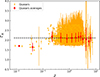 |
Fig. 3. ΓX of the quasar sample and their average values in narrow redshift bins varying with redshifts. |
Although the LX-LUV relation might be redshift-dependent, it is challenging to extract the redshift evolution term due to the degeneracy between the term αlog(1 + z) and the luminosity distance, dL, in Equation (7). As is argued by Lusso et al. (2025), an alternative cosmological model can introduce a redshift-dependent contribution, 2(1 − γ)log dL*(z)/dL(z), where dL(z) and dL*(z) represent the luminosity distances calculated within a fiducial cosmological model and an alternative one, respectively. Fortunately, the luminosity distance-redshift relation has been tightly constrained by the latest BAO measurements from DESI DR2 in combination with CMB and SNe Ia datasets (Abdul Karim et al. 2025). Therefore, the luminosity distance of quasars can be determined with high precision from their measured redshifts and the well-constrained distance-redshift relation. This breaks the degeneracy between αlog(1 + z) and dL in Equation (7), enabling a more robust test of the evolution of the LX-LUV relation.
Figure 4 illustrates the redshift-dependent contributions arising from the choice of cosmological models and datasets, with γ fixed at 0.6. The fiducial cosmological model is the ΛCDM model with parameters constrained by DESI DR2 and CMB data. It is evident that the biases introduced by different cosmological models and datasets are significantly smaller than the redshift-dependent term αlog(1 + z) for z > 0.1. Hence, we can reliably calibrate quasar distance using the fiducial cosmological model without concerns that the αlog(1 + z) term will be overwhelmed by model and dataset selection effects. It should be noted that, to highlight the differences arising from cosmological model and dataset choices, the horizontal axis in Figure 4 is on a logarithmic scale, which gives the impression that αlog(1 + z) grows rapidly with redshift. Actually, the magnitude of αlog(1 + z) is only about 0.6 even at z = 10. Consequently, this term will not produce significant corrections to quasar distances and is unlikely to disrupt the overall consistency between quasar and SNe Ia distance scales at low redshift.
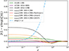 |
Fig. 4. Comparing the redshift-dependence contributions from the cosmological model choice and the term αlog(1 + z). The parameter γ is fixed at 0.6. |
The parameters in the log FX-log FUV relations in Equation (6) and (7) can be inferred from the quasar sample using the Markov chain Monte Carlo (MCMC) code emcee (Foreman-Mackey et al. 2013). The priors for the cosmological parameters were set as H0 = 68.17 ± 0.28 km s−1 Mpc−1 and ΩM = 0.3027 ± 0.0036 with Gaussian probability distributions, where H0 and ΩM were constrained from DESI DR2 in combination with CMB data (Abdul Karim et al. 2025). All other parameters were left unconstrained to avoid imposing artificial biases. The posterior distributions of the parameters in the log FX-log FUV relation were obtained by maximizing the likelihood function
![Mathematical equation: $$ \begin{aligned} \mathcal{{L}} \propto \prod _i \frac{1}{\sqrt{2\pi \sigma _i^2}} \exp \left[-\frac{(y_i-\hat{y}_i)^2}{2\sigma _i^2}\right], \end{aligned} $$](/articles/aa/full_html/2026/02/aa56703-25/aa56703-25-eq12.gif) (11)
(11)
where yi and  denote the observed and modeled values of log FX, respectively. The total measurement error, σi, is composed of the contributions from the uncertainties in log FX and log FUV, expressed as σi2 = σX, i2 + γ2σUV, i2 + δ2, where σX, i and σUV, i are the uncertainties of log FX and log FUV, respectively, and δ accounts for the intrinsic dispersion (Lusso et al. 2020).
The Akaike information criterion (AIC) (Akaike 1974) and the Bayes information criterion (BIC) (Schwarz 1978) are widely used to evaluate models by balancing goodness of fit with model simplicity. They are defined as
 (12)
(12)
 (13)
(13)
where  is the maximum likelihood value, p is the number of free parameters, and N is the number of data. Lower AIC and BIC values indicate a better balance between fit quality and model complexity, implying a more preferable model. In other words, smaller AIC and BIC values correspond to models that fit the quasar data well with lower complexity. So what is truly meaningful is the difference in the AIC and BIC values between a given model and a reference model:
 (14)
(14)
The interpretations of ΔAIC(BIC) are summarized in Table 1.
Interpretations of the differences in AIC and BIC values (Barlow 1990).
3. Analysis and discussion
In this section, we first analyse the dependence of the LX-LUV relation on redshift and on ΓX separately, and then combine the two to discuss the evolution of the LX-LUV relation with respect to both redshift and ΓX simultaneously. All the models are listed in Table 2. Using the MCMC method, the model parameters are constrained from the clean quasar sample (Lusso et al. 2020), and the relative performance of the models is evaluated with the AIC and the BIC.
Different models of LX-LUV relations for quasars.
3.1. The redshift dependence
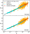 |
Fig. 8. Distance modulus-redshift relations of SNe Ia and quasars. The cyan points are SNe from the Pantheon+ dataset (Scolnic et al. 2022). The orange points are quasars with the non-evo (the upper panel) and evo-zα (the lower panel) models, respectively. The red points are the average distance modulus in narrow redshift bins for quasars only. The dashed black line represents a standard ΛCDM cosmological model with h = H0/(100 km s−1 Mpc−1) = 0.7 and ΩM = 0.3. |
The previous discussion has already provided a specific form for how the LX-LUV relation evolves with redshift in Equation (2), and the parameter α has been estimated to be ∼ 0.57. To more precisely assess the significance of the redshift evolution, the MCMC method introduced in the previous section is employed to constrain the parameters in the LX-LUV relation from the clean quasar sample. For clarity, the standard non-evolutionary LX-LUV relation is referred to as the non-evo model, while the redshift-evolutionary relation is named as evo-zα model, where evo-z denotes the luminosity relation evolving with redshift and α denotes the newly introduced parameter. These models are listed in Table 2. Notably, the evo-zα model reduces to the non-evo model when α = 0.
By fitting the quasar data, the parameter constraints for the non-evo and evo-zα models are shown in Figure 5 and 6, respectively. These figures present the posterior distributions for individual parameters, as well as the two-dimensional joint distributions for parameter pairs. The contours indicate the 1σ and 2σ confidence regions. Notably, the fitted value α = 0.58 ± 0.06 in Figure 6 is consistent with the previous estimate of ∼ 0.57. Furthermore, α deviates from zero at more than 5σ, providing strong evidence for redshift evolution in the LX-LUV relation.
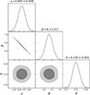 |
Fig. 5. Constraints of the parameters in the non-evo model. |
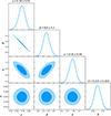 |
Fig. 6. Constraints of the parameters in the evo-zα model. |
Further evidence of this evolution arises from the γ parameter. Figure 7 shows the probability density functions of γ obtained in the model-independent way (the pink one), as well as the non-evo (the grey one) and evo-zα (the blue one) models, respectively. The average value of γ extracted by the model-independent way is ⟨γ⟩ = 0.586 ± 0.061 (Lusso et al. 2020). It is evident that the γ value derived from the non-evo model differs from the model-independent result by about 1σ, whereas the γ value from the evo-zα model is more consistent with the model-independent result. Moreover, the study of Wang et al. (2024) yields the same results, based on the PAge approximation with the clean quasar sample, Pantheon+ SNe Ia data, and H(z) measurements from cosmic chronometers. The reported γ values for the ‘standard’ and ‘Type II’ luminosity relations are 0.655 ± 0.008 and 0.577 ± 0.011, respectively (see Table 2 in the reference). The standard and Type II luminosity relations are equivalent, respectively, to the non-evo and evo-zα models in this work. Therefore, the deviation in γ plausibly indicates redshift evolution in the LX-LUV relation. In addition, the AIC and BIC values for the evo-zα model are 109.0 and 103.2 lower than those for the non-evo model, respectively (see Table 4 and Figure 13). Following the interpretations in Table 1, these results provide very strong evidence in favour of the evo-zα model over the non-evo model.
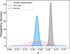 |
Fig. 7. Probability densities of the parameter, γ, obtained in the model-independent way (the pink one), as well as the non-evo (the grey one) and evo-zα (the blue one) models, respectively. |
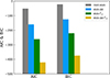 |
Fig. 13. AIC and BIC values for different luminosity models. |
The previous studies have already confirmed that the distance modulus-redshift relation for quasars at z < 1.5 is consistent with that for SNe (Lusso et al. 2019, 2020). To verify that this consistency will not be disrupted after incorporating the redshift-dependent term αlog(1 + z), we compare the distance modulus-redshift relations for SNe Ia and quasars in Figure 8. The cyan points denote the SNe from the Pantheon+ dataset (Scolnic et al. 2022). The distance moduli of quasars estimated with the non-evo and evo-zα models are presented in the upper and lower panels, respectively. The red points represent the average distance modulus in narrow redshift bins for quasars only. We find that the redshift-evolution correction does not introduce any obvious deviation between the quasars and SNe Ia distance moduli. Moreover, accounting for the redshift evolution reduces the dispersion in the quasar data, and there is no longer a significant deviation from the standard cosmological model at high redshift.
3.2. The ΓX dependence
From Equation (2) in the previous section, it can be seen that the LX-LUV relation not only depends on redshift but may also depend on ΓX. To isolate the dependence on ΓX, the LX-LUV relation is assumed to be redshift-independent (i.e. α = 0) in this sub-section.
The ΓX values for the clean quasar sample lie in the range of 1.7 ∼ 2.8, with an average value of ⟨ΓX⟩ = 2.2 (Lusso et al. 2020). We divided the quasar sample into four ΓX bins: 1.7 < ΓX < 2.0, 2.0 < ΓX < 2.2, 2.2 < ΓX < 2.4 and 2.4 < ΓX < 2.8, and fitted each sub-sample with the non-evo model using the MCMC method. The resulting γ and β values are shown in Figure 9. The fits show that γ and β do vary with ΓX and exhibit a coherent linear trend. Specifically, γ increases linearly with ΓX with a slope of 0.13 ± 0.03, while β decreases linearly with ΓX with a slope of −4.1 ± 0.9. Although the growth rate of γ with ΓX appears modest, note that γ is multiplied by log LUV ∼ 30. Therefore, the dependence of both γ and β on ΓX is equally important. In addition, the redshift distributions of the quasar samples in the four ΓX intervals show no obvious differences (Appendix A). This indicates that the ΓX dependence of the LX-LUV relation is not caused by the difference in the redshift distribution, and incorporating the ΓX dependence into the LX-LUV relation is unlikely to induce significant deviations in the cosmological analysis.
Since (ΓX − ⟨ΓX⟩) < 1, γ and β can be approximated by Taylor expansions around ⟨ΓX⟩. Moreover, as we have demonstrated strong linear relations between γ, β and ΓX, it is reasonable to retain only the first-order terms,
 (15)
(15)
 (16)
(16)
where γ0 = γ(⟨ΓX⟩) and β0 = β(⟨ΓX⟩) are the values at the average ⟨ΓX⟩ = 2.2. Focusing only on the ΓX-dependence, we define the model as the evo-ΓX model. The parameter constraints obtained with the MCMC method are shown in Figure 10. Notably, the slope parameters γ1 and β1 are consistent with the previously estimated slopes in Figure 9. The two parameters deviate from zero at approximately 5σ, indicating that the data strongly support a ΓX-dependent relation. γ1 > 0 and β1 < 0 imply a positive correlation between γ(ΓX) and ΓX, and a negative correlation between β(ΓX) and ΓX. Moreover, the AIC and BIC values for the evo-ΓX model are 210.5 and 199.0, which are much lower than the respective ones for the non-evo model (see Table 4 and Figure 13), providing very strong evidence in favour of the evo-ΓX model over the non-evo model. This result indicates that the LX-LUV relation depends on ΓX as well as on SMBH properties.
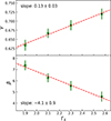 |
Fig. 9. γ and β values obtained by fitting the sub-samples with the non-evo model. |
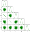 |
Fig. 10. Constraints of the parameters in the evo-ΓX model. |
3.3. Combine the redshift and ΓX dependences
When both redshift and ΓX evolutions were incorporated, we fitted each sub-sample with the evo-zα model; the obtained γ, β, and α values are shown in Figure 11. The figure indicates that γ, β, and α all vary with ΓX. Similarly, although γ increases linearly with ΓX with a slope of 0.04 ± 0.04, the dependencies of γ and β on ΓX are both important, since γ is multiplied by log LUV ∼ 30. However, since α is multiplied by log(1 + z)∈(0, 0.9), the contribution from the ΓX-dependence of α is negligible compared to that of γ and β. Consequently, we continue to consider only the ΓX dependence of γ and β using Equation (15) and (16).
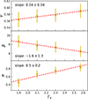 |
Fig. 11. γ and β values obtained by fitting the sub-samples with the evo-zα model. |
The model evo-zα-ΓX was constructed as a combination of the evo-zα model and the evo-ΓX model. The parameter constraints obtained with the MCMC method are shown in Figure 12 and Table 3. The AIC and BIC values for the evo-zα-ΓX model are significantly lower than those for the evo-zα and evo-ΓX models alone, indicating that the joint evolution in redshift and ΓX provides a substantially better fit to the quasar data.
Parameter values for different luminosity relations.
AIC and BIC values for different luminosity models.
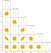 |
Fig. 12. Constraints of the parameters in the evo-zα-ΓX model. |
Finally, it is worth noting that the UV flux of low-redshift (z < 0.7) AGNs is susceptible to contamination from the host galaxy emission (Lusso et al. 2025). Therefore, it is necessary to assess whether our results are influenced by these low-redshift samples. The fact is that the findings remain robust even after excluding the z < 0.7 subset.
4. Conclusions
In this work, the redshift-dependence and ΓX-dependence of the LX-LUV relation are investigated in order to improve distance calibration with quasars. We discuss possible physical origins of these dependences, noting that they are both closely related to the SMBH properties. We provide explicit forms for the redshift and ΓX evolutions. Then the parameters of different luminosity relations are constrained using the clean quasar sample, with quasar distances calibrated by the measurements of DESI DR2 BAO in combination with CMB. Our results strongly favour a model in which the LX-LUV relation evolves simultaneously with redshift and ΓX, and this conclusion is robust irrespective of the choice of cosmological model. In the situation in which the effects of the underlying physical parameters on quasar emissions are not well understood, we adopt a purely data-driven approach to derive an empirical LX-LUV relation that best fits the observed data while maintaining the relation simple. In the future, it will be necessary to combine radiation theory models of quasars with the empirical relations extracted from observations to understand the effects of the underlying physical parameters (such as SMBH mass and accretion rate) on quasar emissions, which, in turn, can improve the distance calibration at high redshift and contribute to our understanding of dark energy.
Acknowledgments
This work was supported by the National Natural Science Foundation of China under grant No. 12405164, No. 12475151, No. U2267205 and No. 12275361, by the Continuous-Support Basic Scientific Research Project under grant No. BJ010261223284, and by the Director Fund of Department of Nuclear Physics in China Institute of Atomic Energy under grant No. 12YA010251223294.
References
- Abdul Karim, M., Aguilar, J., Ahlen, S., et al. 2025, PhRvD, 112, 083515 [Google Scholar]
- Adame, A. G., Aguilar, J., Ahlen, S., et al. 2025, JCAP, 02, 021 [CrossRef] [Google Scholar]
- Aghanim, N., Akrami, Y., Ashdown, M., et al. 2020, A&A, 641, A6 [NASA ADS] [CrossRef] [EDP Sciences] [Google Scholar]
- Akaike, H. 1974, ITAC, 19, 716 [Google Scholar]
- Banados, E., Venemans, B. P., Mazzucchelli, C., et al. 2018, Nature, 553, 473 [NASA ADS] [CrossRef] [Google Scholar]
- Barkhudaryan, L. V., Hakobyan, A. A., Karapetyan, A. G., et al. 2019, MNRAS, 490, 718 [NASA ADS] [CrossRef] [Google Scholar]
- Barlow, R. J. 1990, NIMA, 297, 496 [Google Scholar]
- Bisogni, S., Lusso, E., Civano, F., et al. 2021, A&A, 655, A109 [NASA ADS] [CrossRef] [EDP Sciences] [Google Scholar]
- Bravo, E., Dominguez, I., Badenes, C., Piersanti, L., & Straniero, O. 2010, ApJ, 711, L66 [NASA ADS] [CrossRef] [Google Scholar]
- Breuval, L., Riess, A. G., Casertano, S., et al. 2024, ApJ, 973, 30 [Google Scholar]
- Brightman, M., Silverman, J. D., Mainieri, V., et al. 2013, MNRAS, 433, 2485 [Google Scholar]
- Childress, M. J., Aldering, G., Antilogus, P., et al. 2013, ApJ, 770, 108 [NASA ADS] [CrossRef] [Google Scholar]
- Connolly, S. D., McHardy, I. M., Skipper, C. J., & Emmanoulopoulos, D. 2016, MNRAS, 459, 3963 [CrossRef] [Google Scholar]
- Fausnaugh, M. M., Denney, K. D., Barth, A. J., et al. 2016, ApJ, 821, 56 [Google Scholar]
- Foreman-Mackey, D., Hogg, D. W., Lang, D., & Goodman, J. 2013, PASP, 125, 306 [Google Scholar]
- Freedman, W. L., Madore, B. F., Hoyt, T. J., et al. 2025, ApJ, 985, 203 [Google Scholar]
- Gu, M., & Cao, X. 2009, MNRAS, 399, 349 [NASA ADS] [CrossRef] [Google Scholar]
- Haardt, F., & Maraschi, L. 1993, ApJ, 413, 507 [Google Scholar]
- Hagstotz, S., Reischke, R., & Lilow, R. 2022, MNRAS, 511, 662 [CrossRef] [Google Scholar]
- Hicken, M., Wood-Vasey, W. M., Blondin, S., et al. 2009, ApJ, 700, 1097 [Google Scholar]
- Jha, S., Riess, A. G., & Kirshner, R. P. 2007, ApJ, 659, 122 [NASA ADS] [CrossRef] [Google Scholar]
- Johansson, J., Thomas, D., Pforr, J., et al. 2013, MNRAS, 435, 1680 [CrossRef] [Google Scholar]
- Jones, D. O., Riess, A. G., Scolnic, D. M., et al. 2018, ApJ, 867, 108 [NASA ADS] [CrossRef] [Google Scholar]
- Kang, Y., Lee, Y.-W., Kim, Y.-L., Chung, C., & Ree, C. H. 2020, ApJ, 889, 8 [Google Scholar]
- Kelly, B. C., Bechtold, J., Trump, J. R., Vestergaard, M., & Siemiginowska, A. 2008, ApJS, 176, 355 [Google Scholar]
- Kelly, P. L., Hicken, M., Burke, D. L., Mandel, K. S., & Kirshner, R. P. 2010, ApJ, 715, 743 [Google Scholar]
- Kim, Y., Smith, M., Sullivan, M., & Lee, Y. 2018, ApJ, 854, 24 [NASA ADS] [CrossRef] [Google Scholar]
- Lee, Y.-W., Chung, C., Kang, Y., & Jee, M. J. 2020, ApJ, 903, 22 [Google Scholar]
- Li, G. X., & Li, Z. H. 2021, AJ, 162, 249 [Google Scholar]
- Li, Z., Huang, L., & Wang, J. 2022, MNRAS, 517, 1901 [Google Scholar]
- Li, X., Keeley, R. E., & Shafieloo, A. 2025, ApJ, 983, 141 [Google Scholar]
- Liu, Y., Yu, H., & Wu, P. 2023, ApJ, 946, L49 [NASA ADS] [CrossRef] [Google Scholar]
- Lusso, E., & Risaliti, G. 2017, A&A, 602, A79 [NASA ADS] [CrossRef] [EDP Sciences] [Google Scholar]
- Lusso, E., Piedipalumbo, E., Risaliti, G., et al. 2019, A&A, 628, L4 [NASA ADS] [CrossRef] [EDP Sciences] [Google Scholar]
- Lusso, E., Risaliti, G., Nardini, E., et al. 2020, A&A, 642, A150 [NASA ADS] [CrossRef] [EDP Sciences] [Google Scholar]
- Lusso, E., Risaliti, G., & Nardini, E. 2025, A&A, 697, A108 [NASA ADS] [CrossRef] [EDP Sciences] [Google Scholar]
- Murakami, Y. S., Stahl, B. E., Zhang, K. D., et al. 2021, MNRAS, 504, L34 [Google Scholar]
- Perlmutter, S., Gabi, S., Goldhaber, G., et al. 1997, ApJ, 483, 565 [Google Scholar]
- Perlmutter, S., Aldering, G., Goldhaber, G., et al. 1999, ApJ, 517, 565 [Google Scholar]
- Ricci, C., Ho, L. C., Fabian, A. C., et al. 2018, MNRAS, 480, 1819 [NASA ADS] [CrossRef] [Google Scholar]
- Riess, A. G., Press, W. H., & Kirshner, R. P. 1996, ApJ, 473, 88 [Google Scholar]
- Riess, A. G., Filippenko, A. V., Challis, P., et al. 1998, AJ, 116, 1009 [Google Scholar]
- Riess, A. G., Casertano, S., Yuan, W., Macri, L. M., & Scolnic, D. 2019, ApJ, 876, 85 [Google Scholar]
- Riess, A. G., Yuan, W., Macri, L. M., et al. 2022, ApJ, 934, L7 [NASA ADS] [CrossRef] [Google Scholar]
- Riess, A. G., Anand, G. S., Yuan, W., et al. 2024, ApJ, 962, L17 [NASA ADS] [CrossRef] [Google Scholar]
- Rigault, M., Aldering, G., Kowalski, M., et al. 2015, ApJ, 802, 20 [Google Scholar]
- Rigault, M., Brinnel, V., Aldering, G., et al. 2020, A&A, 644, A176 [NASA ADS] [CrossRef] [EDP Sciences] [Google Scholar]
- Risaliti, G., & Lusso, E. 2015, ApJ, 815, 33 [NASA ADS] [CrossRef] [Google Scholar]
- Risaliti, G., & Lusso, E. 2017, Astron. Nachr., 338, 329 [NASA ADS] [CrossRef] [Google Scholar]
- Risaliti, G., & Lusso, E. 2019, NatAs, 3, 272 [Google Scholar]
- Risaliti, G., Young, M., & Elvis, M. 2009, ApJ, 700, L6 [NASA ADS] [CrossRef] [Google Scholar]
- Roman, M., Hardin, D., Betoule, M., et al. 2018, A&A, 615, A68 [NASA ADS] [CrossRef] [EDP Sciences] [Google Scholar]
- Rose, B. M., Garnavich, P. M., & Berg, M. A. 2019, ApJ, 874, 32 [Google Scholar]
- Rose, B. M., Rubin, D., Cikota, A., et al. 2020, ApJ, 896, L4 [Google Scholar]
- Rybicki, G. B., & Lightman, A. P. 1979, Radiative Processes in Astrophysics (New York: Wiley) [Google Scholar]
- Salvestrini, F., Risaliti, G., Bisogni, S., Lusso, E., & Vignali, C. 2019, A&A, 631, A120 [NASA ADS] [CrossRef] [EDP Sciences] [Google Scholar]
- Schmidt, B. P., Suntzeff, N. B., Phillips, M. M., et al. 1998, ApJ, 507, 46 [NASA ADS] [CrossRef] [Google Scholar]
- Schwarz, G. 1978, Ann. Stat., 6, 461 [Google Scholar]
- Scolnic, D., Brout, D., Carr, A., et al. 2022, ApJ, 938, 113 [NASA ADS] [CrossRef] [Google Scholar]
- Shemmer, O., Brandt, W. N., Netzer, H., Maiolino, R., & Kaspi, S. 2008, ApJ, 682, 81 [Google Scholar]
- Signorini, M., Risaliti, G., Lusso, E., et al. 2024, A&A, 687, A32 [NASA ADS] [CrossRef] [EDP Sciences] [Google Scholar]
- Sullivan, M., Conley, A., Howell, D. A., et al. 2010, MNRAS, 406, 782 [NASA ADS] [Google Scholar]
- Suzuki, N., Rubin, D., Lidman, C., et al. 2012, ApJ, 746, 85 [NASA ADS] [CrossRef] [Google Scholar]
- Tananbaum, H., Avni, Y., Branduardi, G., et al. 1979, ApJ, 234, L9 [Google Scholar]
- Timmes, F., Brown, E. F., & Truran, J. 2003, ApJ, 590, L83 [Google Scholar]
- Trefoloni, B., Lusso, E., Nardini, E., et al. 2024, A&A, 689, A109 [NASA ADS] [CrossRef] [EDP Sciences] [Google Scholar]
- Wang, B., Liu, Y., Yuan, Z., et al. 2022, ApJ, 940, 174 [Google Scholar]
- Wang, B., Liu, Y., Yu, H., & Wu, P. 2024, ApJ, 962, 103 [Google Scholar]
- Wu, Q., Zhang, G.-Q., & Wang, F.-Y. 2022, MNRAS, 515, L1 [NASA ADS] [CrossRef] [Google Scholar]
- Wu, J., Liu, Y., Yu, H., & Wu, P. 2025, CPC, 49, 075101 [Google Scholar]
Appendix A: The redshift distributions in different ΓX intervals
In Section 3.2, we divided the quasar samples into four ΓX intervals: 1.7 < ΓX < 2.0, 2.0 < ΓX < 2.2, 2.2 < ΓX < 2.4 and 2.4 < ΓX < 2.8, and examined the ΓX dependence of the LX-LUV relation. If the redshift distribution differs significantly across the four ΓX intervals, such a discrepancy could bias the cosmological analysis.
Figure A.1 presents the redshift distributions of the quasar samples in the four ΓX intervals. The distributions show no obvious differences. We also examined the mean redshifts and their standard deviations for the samples in the four ΓX intervals. Figure A.2 uses the entire dataset within the redshift range 0.009 < z < 7.52, while Figure A.3 uses only the sub-sample within the redshift range 0.5 < z < 2.5, where the number statistics are sufficient. Linear fits for both cases indicate no significant difference in redshift across the four ΓX intervals. This implies that the distribution of ΓX does not depend on the chosen redshift interval. In other words, there is no preference for steeper or softer ΓX as a function of the sample redshift. Therefore, for the adopted quasar dataset, the introduction of the ΓX dependence of the LX-LUV relation will not lead to significant deviations in the cosmological analysis.
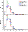 |
Fig. A.1. The redshift distributions of the quasar samples in the four ΓX intervals: 1.7 < ΓX < 2.0, 2.0 < ΓX < 2.2, 2.2 < ΓX < 2.4 and 2.4 < ΓX < 2.8. The vertical axis in the upper panel represents the number of samples, while the vertical axis in the lower panel represents the normalized number of samples. |
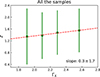 |
Fig. A.2. The mean redshifts and their standard deviations for the samples in the four ΓX intervals. All the quasar samples within the redshift range 0.009 < z < 7.52 are employed. |
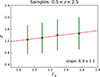 |
Fig. A.3. The mean redshifts and their standard deviations for the samples in the four ΓX intervals. Only the sub-sample within the redshift range 0.5 < z < 2.5 are employed. |
All Tables
All Figures
|
Fig. 1. UV and X-ray monochromatic luminosities of quasars in different redshift intervals. The luminosities were obtained from the measured fluxes assuming a standard ΛCDM cosmological model with H0 = 70 km s−1 Mpc−1 and ΩM = 0.3. |
| In the text | |
|
Fig. 2. UV (the upper panel) and X-ray (the lower panel) monochromatic luminosities (in units of erg s−1 Hz−1) of quasars varying with redshifts. The luminosities were obtained from the measured fluxes assuming a standard ΛCDM cosmological model with H0 = 70 km s−1 Mpc−1 and ΩM = 0.3. The log LUV(X) approximately linearly increases with log(1 + z) within the range of redshifts where the statistical quantity of sample is sufficient. The dashed red lines are the optimal linear fits, and kUV(X) are the corresponding slopes. |
| In the text | |
|
Fig. 3. ΓX of the quasar sample and their average values in narrow redshift bins varying with redshifts. |
| In the text | |
|
Fig. 4. Comparing the redshift-dependence contributions from the cosmological model choice and the term αlog(1 + z). The parameter γ is fixed at 0.6. |
| In the text | |
|
Fig. 8. Distance modulus-redshift relations of SNe Ia and quasars. The cyan points are SNe from the Pantheon+ dataset (Scolnic et al. 2022). The orange points are quasars with the non-evo (the upper panel) and evo-zα (the lower panel) models, respectively. The red points are the average distance modulus in narrow redshift bins for quasars only. The dashed black line represents a standard ΛCDM cosmological model with h = H0/(100 km s−1 Mpc−1) = 0.7 and ΩM = 0.3. |
| In the text | |
|
Fig. 5. Constraints of the parameters in the non-evo model. |
| In the text | |
|
Fig. 6. Constraints of the parameters in the evo-zα model. |
| In the text | |
|
Fig. 7. Probability densities of the parameter, γ, obtained in the model-independent way (the pink one), as well as the non-evo (the grey one) and evo-zα (the blue one) models, respectively. |
| In the text | |
|
Fig. 13. AIC and BIC values for different luminosity models. |
| In the text | |
|
Fig. 9. γ and β values obtained by fitting the sub-samples with the non-evo model. |
| In the text | |
|
Fig. 10. Constraints of the parameters in the evo-ΓX model. |
| In the text | |
|
Fig. 11. γ and β values obtained by fitting the sub-samples with the evo-zα model. |
| In the text | |
|
Fig. 12. Constraints of the parameters in the evo-zα-ΓX model. |
| In the text | |
|
Fig. A.1. The redshift distributions of the quasar samples in the four ΓX intervals: 1.7 < ΓX < 2.0, 2.0 < ΓX < 2.2, 2.2 < ΓX < 2.4 and 2.4 < ΓX < 2.8. The vertical axis in the upper panel represents the number of samples, while the vertical axis in the lower panel represents the normalized number of samples. |
| In the text | |
|
Fig. A.2. The mean redshifts and their standard deviations for the samples in the four ΓX intervals. All the quasar samples within the redshift range 0.009 < z < 7.52 are employed. |
| In the text | |
|
Fig. A.3. The mean redshifts and their standard deviations for the samples in the four ΓX intervals. Only the sub-sample within the redshift range 0.5 < z < 2.5 are employed. |
| In the text | |
Current usage metrics show cumulative count of Article Views (full-text article views including HTML views, PDF and ePub downloads, according to the available data) and Abstracts Views on Vision4Press platform.
Data correspond to usage on the plateform after 2015. The current usage metrics is available 48-96 hours after online publication and is updated daily on week days.
Initial download of the metrics may take a while.