| Issue |
A&A
Volume 706, February 2026
|
|
|---|---|---|
| Article Number | A123 | |
| Number of page(s) | 10 | |
| Section | The Sun and the Heliosphere | |
| DOI | https://doi.org/10.1051/0004-6361/202556749 | |
| Published online | 04 February 2026 | |
Inference of the physical parameters of Hα-absorbing plasma structures in the quiet Sun
1
Astronomy Program, Department of Physics and Astronomy, Seoul National University Gwanak-gu Seoul 08826, Republic of Korea
2
Astronomy Research Center, Seoul National University Gwanak-gu Seoul 08826, Republic of Korea
3
Korea Astronomy and Space Science Institute, Daedeokdae-ro Yuseong-gu Daejeon 34055, Republic of Korea
4
Max-Planck Institute for Solar System Research Justus-von-Liebig-Weg 3 37077 Göttingen, Germany
5
Space Research and Technology Institute, Bulgarian Academy of Sciences, Acad. Georgy Bonchev Str. Bl. 1 1113 Sofia, Bulgaria
6
Research Institute of Natural Sciences, Chungnam National University, 99 Daehak-ro Yuseong-gu Daejeon 34134, Republic of Korea
7
Astronomy and Space Science, University of Science and Technology, 217 Gajeong-ro Yuseong-gu Daejeon 34113, Republic of Korea
★ Corresponding author: This email address is being protected from spambots. You need JavaScript enabled to view it.
Received:
5
August
2025
Accepted:
27
November
2025
Abstract
On-disk Hα light-absorbing plasma structures such as mottles, fibrils, filaments, and Hα jets are observable magnetohydrodynamic features in the upper solar chromosphere. We attempt to determine their physical parameters by regarding them as optical clouds scattering the Hα-line light incident from below. For this purpose, we developed a new inversion, which we call the three-layer background plus three-component cloud model inversion. This new spectral inversion was found to be applicable to every Hα line profile taken from a quiet-Sun region. We used the model parameters inferred from the fitting to determine the temperature and to construct the velocity distribution function at every point in the observed region. This function was used in turn to calculate the column mass, mass flux, kinetic energy, and kinetic energy flux. Our approach yielded three types of Doppler velocities: the mass flux-associated velocity, the kinetic energy-associated velocity, and the kinetic energy flux-associated velocity. We found that the physical parameters of Hα-absorbing structures in a quiet-Sun region resolve the long-standing discrepancy between the Doppler velocities of mottles observed on the disk and the rising speeds of spicules observed off the limb. We also found that the kinetic energy budget of the upper chromosphere is large enough for the radiative loss in the upper chromosphere and corona. These results support the hypothesis that magnetohydrodynamic waves heat the upper atmosphere of the quiet Sun.
Key words: line: profiles / magnetohydrodynamic (MHD) / plasmas / Sun: chromosphere
© The Authors 2026
 Open Access article, published by EDP Sciences, under the terms of the Creative Commons Attribution License (https://creativecommons.org/licenses/by/4.0), which permits unrestricted use, distribution, and reproduction in any medium, provided the original work is properly cited.
This article is published in open access under the Subscribe to Open model. This email address is being protected from spambots. You need JavaScript enabled to view it. to support open access publication.
1. Introduction
High-resolution Hα observations of a quiet region on the solar disk reveal a variety of Hα-absorbing plasma structures, such as mottles, fibrils, grains, filaments, and jets (Tsiropoula et al. 2012). They appear to be darker than the background atmosphere because they are located higher above the background atmosphere, which scatters the Hα light (Leenaarts et al. 2012; Pereira et al. 2012; Bate et al. 2022). These features can stay high either because they are magnetically supported, as in filaments (Foukal 1971), or because they move at fast speeds, as in mottles (e.g., Suematsu et al. 1995), fibrils (e.g., De Pontieu et al. 2007), and jets (e.g., Langangen et al. 2008). These Hα-absorbing features are a natural outcome of magnetohydrodynamic activity in the solar chromosphere. To understand the physics of these features, it is crucial to determine their physical parameters and to characterize their morphology in space and time. Observational studies of the proper determination of the physical parameters (e.g., Tsiropoula & Schmieder 1997; Tsiropoula & Tziotziou 2004) are still scarce, however, and this scarcity remains an obstacle to clarifying the physical nature and role of Hα-absorbing features.
A long-standing puzzle is that when they are observed on the disk, the Doppler velocities of these Hα features are estimated to be much lower than expected. Grossmann-Doerth & Von Uexküll (1971) determined the Doppler velocities of Hα mottles, which are the supposed disk-counterpart of limb spicules, by applying Beckers’s cloud model (Beckers 1964). As a result, they found that disk mottles are similar to the limb spicules described by Beckers (1968) in optical thickness, source function, and Doppler width, but their Doppler velocities, with a mean absolute value of 3.9 km s−1, were much lower than those expected from the rising motion of spicules seen above the limb. This result for the Doppler velocity measurements of mottles was confirmed by subsequent studies that indicated mean absolute values lower than 6 km s−1 (e.g, Tsiropoula et al. 1993; Tziotziou et al. 2003). The Doppler velocities determined with the lambdameter method (e.g., Chae et al. 2014) are even lower than those determined from the cloud model; their maximum absolute values are lower than 4 km s−1.
These Doppler observations differ from imaging observations with a high angular resolution and high temporal resolution that often revealed high-velocity motions on the plane of sky from the paths of mottle tops or fibril tops. Suematsu et al. (1995) obtained a mean of 18 km s−1 for the time-averaged velocities from the disk spicules (actually mottles) in an enhanced network area, and Rouppe van der Voort et al. (2007) derived the maximum velocities in the range of 10–30 km s−1 from the mottles in the quiet Sun. Hansteen et al. (2006) obtained maximum velocities in the range of 10–40 km s−1 from dynamic fibrils in active regions, which are similar to mottles in the quiet Sun. These observations support the hypothesis that mottles (or fibrils) are the disk counterpart of limb spicules (e.g., Grossmann-Doerth & Von Uexküll 1973; Suematsu et al. 1995; Pereira et al. 2016). Nevertheless, the discrepancy between Doppler velocity measurements and plane-of-sky velocity measurements remains unresolved.
Hα-absorbing plasma structures may be regarded as optical clouds that scatter the Hα-line light incident from below. A well-developed cloud model might therefore be used to characterize the physical properties of these plasma structures. A few problems arise when the conventional cloud models are applied to the Hα spectral data of Hα-absorbing features, however. First, the performance of the cloud model strongly depends on the chosen background intensity profile, and it is hard to choose this profile correctly. The background intensity profile is usually obtained from the region next to the projected dark structure or from the spatial average of the observed line profiles over a given region. This is the most popular application of the cloud model and is often referred to as the classical cloud model or Beckers’s cloud model (BCM, Beckers 1964). The BCM typically works well in high-lying clouds (e.g., filaments), but it fails in some low-lying clouds (e.g., Hα dark grains) because the adopted background intensity profile significantly deviates from the real background profile. The embedded cloud model (ECM) developed by Chae (2014) partially resolved this problem by setting the background light to the ensemble-average light at the same height, but it is still not satisfactory enough. The next problem is that the cloud model with a single-Gaussian component absorption often fails to fit the observational data. This is expected because there is a good possibility that more than one cloud is located along the line of sight at a given position, with each cloud moving at its own velocity.
Finally, the inference of the physical parameters such as mass and kinetic energy from the cloud model parameters is not yet well established. A pioneering work in this type of topic was made by Tsiropoula & Schmieder (1997). They inferred not only the temperature and hydrogen populations, but also the total hydrogen density and hydrogen ionization from the cloud model parameters. Their inference of the total hydrogen density and hydrogen ionization heavily depends on the results of non-local thermodynamic equilibrium (non-LTE) radiative solutions obtained in a specific geometry, however, and the temperature determined from the Doppler width was unrealistically large in a number of measurements. Tsiropoula & Tziotziou (2004) calculated the contribution of mottles to the mass flux and kinetic energy flux by adopting typical values of the mass density, the areal filling factor of mottles, and the axis velocity. These adopted parameters are not directly related to the cloud model parameters, however. Al et al. (2004) provided an estimate of kinetic energy flux in an enhanced network region from the mean value of the line-of-sight velocity, which is one of the cloud model parameters. This approach produced a kinetic energy flux far lower than required for the radiative loss because high-velocity plasma is not well considered when the velocity is distributed over a range.
We intend to determine the physical parameters of Hα-absorbing features by solving the three problems mentioned above. First, we specify the intensity profile of light incident from below at each point in a self-consistent way. We identify this intensity profile with the line profile of the light emerging from the conventional chromosphere, which is modeled by three layers in the scheme of the multilayer spectral inversion (MLSI) developed by Chae et al. (2020) and Chae et al. (2021). Essentially, the intensity profile of the incident light is not given a priori, but is to be determined from the model. Second, the optical thickness profile is modeled by the sum of three Gaussian components, which we find is general enough to fit a variety of observed line profiles. Finally, we define the velocity distribution function based on the cloud model parameters. This velocity distribution is used to calculate the column mass, column kinetic energy, column kinetic energy flux, and so on.
2. Method
2.1. Three-layer background plus three-component cloud model inversion
We propose a slightly sophisticated spectral inversion model: A model of a cloud with three velocity components above a three-layer background atmosphere. This model is a generalized version of the multilayer spectral inversion (MLSI) developed by Chae et al. (2020) and Chae et al. (2021). We modeled the background atmosphere by introducing three layers: one layer for the photosphere, and two layers for the chromosphere, as in Chae et al. (2021). The background chromosphere was assumed to be stationary. We regarded the highest part of the atmosphere as a cloud located above the background atmosphere. Unlike the background atmosphere, this cloud can move at significant speeds. Furthermore, this cloud can have subcomponents, each of which moves at its own velocity. We modeled the velocity distribution inside a cloud by superposing three Gaussian velocity components.
Our inversion model looks similar to the classical cloud model. The line intensity profile Iλ observed at a specified position on the solar disk is theoretically given by the form
![Mathematical equation: $$ \begin{aligned} I_\lambda = I_{\lambda , 0} (\mathbf p _0) \exp (-\tau _\lambda (\mathbf p _c) ) + S \left[ 1- \exp (-\tau _\lambda (\mathbf p _c) ) \right], \end{aligned} $$](/articles/aa/full_html/2026/02/aa56749-25/aa56749-25-eq1.gif) (1)
(1)
where the background intensity profile of the incident light Iλ, 0 is specified by a parameter set p0, and the source function S and the optical thickness profile τλ of the cloud are given by another parameter set pc.
The background intensity Iλ, 0(p0) at a point is identified with the intensity emerging from the background atmosphere modeled by three layers. Chae et al. (2021) specified all the elements of p0 in detail, and six of these parameters are relevant to the current work: the velocities v0 and v1, Doppler widths w0 and w1, and the source functions S0 and S1 at the outer boundary and the inner interface of the upper chromosphere. We set v0 and v1 to zero and practically fixed w0 and w1 to the prescribed values (0.40 Å and 0.36 Å) because the background atmosphere was assumed to be static. The main parameters of p0 to be determined from the model fit are then S0 and S1.
We assumed that the absorption feature consisted of a finite number of moving clouds so that the Hα optical thickness profile is given by
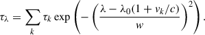 (2)
(2)
Here, λ0 is the laboratory wavelength of the line, and c is the speed of light. From now on, the subscript k denotes one of the subscripts b (blueshifted component), c (central component), and r (redshifted component). A similar three-velocity component analysis of an Hα-absorbing cloud was previously reported by Chae et al. (2007), who studied the dynamics in a filament. Unlike this previous study, we focused not on the individual velocity components, but on the parameters resulting from the integration of all the velocity components. For example, we obtained the total optical thickness by simply summing all the contributions,
 (3)
(3)
For simplicity, we assumed that the Doppler width was the same for all the velocity components. The cloud model is thus described by pc, a set of eight free parameters: the source function S, the Doppler width w, the optical depth τb, and the velocity vb of the blueshifted (or upward-moving) component, τc and the velocity vc of the central (or slowly moving) component, and τr and vr of the redshifted (or downward-moving) component.
We recall that Iλ and Iλ, 0 are the theoretical line profiles. From the observations, we obtained the observed line profile Iλ,obs. We also usually obtained the reference background intensity profile Iλ,ref by spatially averaging all the profiles inside the field of view. We required that Iλ,obs was to be fit by Iλ in a tight way, and Iλ,ref was to be fit by Iλ, 0 in a loose way. These two fittings were made simultaneously by minimizing the functional
![Mathematical equation: $$ \begin{aligned} H \equiv \frac{1}{N} \sum _\lambda \left[ \left(\frac{I_{\lambda }-I_{\lambda , \mathrm {obs}}}{\sigma _\lambda } \right)^2 + \left(\frac{I_{\lambda ,0}-I_{\lambda , \mathrm {ref}}}{5\sigma _\lambda }\right)^2 \right] + \left[ \epsilon _D (\mathbf p _0, \mathbf p _c) \right]^2, \end{aligned} $$](/articles/aa/full_html/2026/02/aa56749-25/aa56749-25-eq4.gif) (4)
(4)
where σλ is the standard error in the observed profile at each wavelength, and N is the number of the sampled wavelengths. The last term on the right side denotes the sum of penalty functions constraining the parameters p0 and pc, as was employed by Chae et al. (2021). The last term also includes the constraint that w has to be in a specified range, for example, between 0.25 Å and 0.44 Å, corresponding to the values obtained with the temperature range between 4000 K and 20 000 K and the nonthermal broadening ξ = 8 km s−1. We found this constraint is helpful to stably obtain a physically reasonable fitting.
Our model fitting is characterized by ten free parameters. The two parameters S0 and S1 constitute p0, and the eight parameters S, w, τb, τc, τr, vb, vc, and vr constitute pc.
2.2. Physical parameters
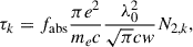
The temperature T can be reasonably determined from w using the formula
![Mathematical equation: $$ \begin{aligned} T = \frac{m_{\rm {H}} }{2 k_{\rm B}} \left[ \left( c \frac{w}{\lambda _0}\right)^2 - \xi ^2 \right] \end{aligned} $$](/articles/aa/full_html/2026/02/aa56749-25/aa56749-25-eq5.gif) (5)
(5)
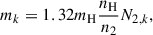
if the speed of nonthermal motion ξ is specified. Here, mH is the hydrogen mass, and kB is the Boltzmann constant.
According to Chae et al. (2021), who analyzed the Ca II 8542 Å line data as well as the Hα line data, the nonthermal motion ξ ranges from 7.5 to 8.9 km s−1 in the quiet Sun. We therefore adopted ξ = 8 km s−1 because ξ of individual features cannot be independently determined with the Hα line data alone. We estimated the contribution to ξ2 by the instrumental broadening of the FISS data at 1.4 km2 s−2, which is much smaller than 64 km2 s−2.
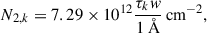
The optical thickness τk is related to the oscillator strength of the line absorption fabs, the electron charge e, the electron mass me, and the column number density N2, k (in cm−2) of hydrogen in the first excited (n = 2) level via
 (6)
(6)
where the effect of the induced emission was neglected because the ratio of the upper-level population to the lower-level population is quite low in the solar chromosphere (see, e.g., Vernazza et al. 1981). From the above equation, we obtained the expression of the column density of n = 2 hydrogen of the kth cloud,
 (7)
(7)
and its total column density,
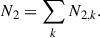 (8)
(8)
The column mass density of the kth cloud mk in g cm−2 is then given by
 (9)
(9)
where n2 and nH are the n = 2 hydrogen population and the total (neutral + ionized) hydrogen population in cm−3. This equation was combined with Eq. (7) to yield
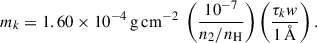 (10)
(10)
We next determined n2/nH. This ratio was reported to be not very sensitive to local physical conditions in the upper chromosphere (Leenaarts et al. 2012). This weak sensitivity arises because the ionization and excitation are much more affected by radiation than by collision there. By solving the 3D radiative transfer in the simulated chromosphere, Leenaarts et al. (2012) produced the probability distribution function of n2/nH, which slowly varies with temperature at heights between 1 Mm and 3 Mm. We obtained from this function the empirical approximations
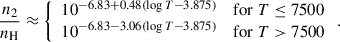 (11)
(11)
We then defined the velocity function. The infinitesimal column mass dm(v) that moves in the line-of-sight direction velocity in the infinitesimal range v from v + dv is given by
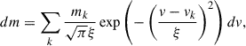 (12)
(12)
based on which, we defined the velocity distribution function as
 (13)
(13)
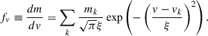
v here refers to the plasma motion (including the plasma bulk motion and unresolved nonthermal motion, but excluding the molecular thermal motion). Its sign is defined to be negative for the motion approaching the observer and positive for the motion receding from the observer. This velocity distribution function was exploited to derive the zeroth-order moment of v (column mass),
 (14)
(14)
the first-order moment (column mass flux),
 (15)
(15)
the second-order moment (column kinetic energy),
 (16)
(16)
and the third-order moment (column kinetic energy flux),
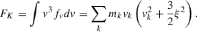 (17)
(17)
We recall that EK and FK have a contribution from the nonthermal speed ξ as well as the bulk motion velocity vk. We also note that in the definition of EK, the numeric factor 1 has been used instead of 1/2, which means that EK was defined by twice the kinetic energy contributed by the line-of-sight or longitudinal velocity component. By assuming that the contribution of the transverse velocity component is the same as that of the longitudinal component, we can regard EK as the total kinetic energy equally contributed by the longitudinal and the transverse component. In a similar way, FK can be regarded as the longitudinal flux of the total kinetic energy.
In addition, we defined the first-order moment velocity
 (18)
(18)
which is related to the mass flux, the second-order moment velocity
 (19)
(19)
which is related to the kinetic energy, and the third-order moment velocity,
 (20)
(20)
which is related to the kinetic energy flux. vE has a contribution from the nonthermal speed ξ as well as the bulk motion velocity vk, and it is always positive, whereas vM and vF are either positive or negative. The negative values indicate motions that are directed upward, which is toward the observer on the Earth.
The mass density ρ and number density n2 can be determined from the relations
 (21)
(21)
 (22)
(22)
when the vertical extent H is known. The determination of the vertical extent H at every position is practically impossible. Therefore, we fixed H to the value 1.4H0, where H0 ≡ 360 km is the pressure scale height estimated from a typical temperature of 8000 K and a typical nonthermal motion of 8 km s−1. The factor 1.4 was taken from the estimated average number of structures on the line of sight (see Sect. 4.3).
2.3. Error estimates
We estimated the statistical errors of the model parameters and the derived physical parameters based on a Monte Carlo simulation. For a given observed profile Iλ,obs, we constructed an ensemble of 100 profiles: Iλ,obs,j ≡ Iλ,obs + nλ,j for j = 1, ..., 100, where nλ, j is the noise of the jth profile at a wavelength λ that was randomly generated with a normal distribution of the zero mean and the given standard error σλ that was used in Eq. (4). We adopted the Poisson standard noise  . By applying the model fit to every profile in the ensemble, we obtained 100 sets of the model parameters and the derived physical parameters. The standard deviation in each parameter was regarded as the statistical error of the parameter. The systematic errors can only be estimated when the solution is known.
3. Validation test using simulation data
In order to estimate the systematic errors, we performed a validation test using the synthetic Hα intensity profiles and 3D arrays of vertical velocity, temperature, and hydrogen populations taken from the 3D radiative MHD simulation of Leenaarts et al. (2012). By applying our three-layer-plus-cloud model inversion to the synthetic intensity profiles, we inferred the line-of-sight velocity, temperature, and hydrogen population in the first excited state and the mass density, and we compared them with the simulation values at two specified heights.
The synthetic Hα data differ from real observations in a couple of ways. Their images look similar to the observations in that they display dark fibril-like structures that are as thick as the observed fibrils, but the fibrils in the simulation appear to be shorter and less densely packed than the fibrils seen in the real observations, as described by Leenaarts et al. (2012). In addition, the synthetic Hα line profiles are much narrower than the observations for reasons that are not yet understood. This type of difference in the line width between simulations and observations also occurs in the resonance lines, for instance, in the Mg II lines. Recent theoretical studies (Judge et al. 2020; Hansteen et al. 2023) suggested that nonthermal motions alone might not account for the difference in the width of Mg II lines and that other effects such as horizontal radiative transfer might be important.
We adapted our inversion model to the synthetic line profiles. First, we found that when we used only one velocity component in the cloud, the fit was fairly satisfactory in most cases and the analysis became simple. Second, we set w0 and w1 to 0.25 Å, which is lower than what we used to invert the real observations. Third, we set ξ to 3 km s−1, which is lower than the 8 km s−1 we used to invert the real observations. This value of 3 km s−1 was chosen so that the inferred temperatures became comparable to the simulation values. It mainly accounts for the nonthermal broadening originating in the varying line-of-sight velocity.
Figure 1a illustrates that our inversion model fits the synthetic line profiles well. In this specific case, the model background intensity I0 is found to be very close to the mean synthetic line profile. The inversion produced the physical parameters line-of-sight velocity v, temperature T, and n = 2 hydrogen population n2, which are marked by horizontal red lines in Figs. 1b, 1c, and 1d, respectively. n2 was calculated by dividing the inferred column density N2 by the assumed vertical extent H = 500 km. These values are compared with the simulation values at two reference heights. One reference height is set to the height of the cloud zc, which is defined by the height where the simulation value of the column number N2, accumulated from above is equal to half the inferred value N2. The other height is defined by height z1 at which the Hα line core is formed, which is obtained from the result of the 3D radiative MHD simulation. In many cases, these two heights are close to each other. The figure indicates that the inversion values of v, T, and n2 are close to the simulation values at these heights. In this specific example, the match between the inversion and the simulation is satisfactory.
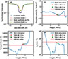 |
Fig. 1. Inversion model fit to a synthetic Hα line profile of an absorption feature. |
Figure 2 compares the parameters of the nine absorption features inferred from the inversion and the values taken from the simulation at the two reference heights. The line-of-sight velocity v matches well. The mean absolute difference is about 1 km s−1. For the temperature, Fig. 2b shows that the match is moderately good; the mean absolute difference is about 1000 K. Figure 2c indicates that the inversion values of log n2 match the simulation values at z = z1 with a mean absolute difference of 0.50 and with those at z = zc with a mean absolute difference of 0.26. Similarly, Fig. 2d indicates that the inversion values of log ρ match the simulation values at z = z1 with a mean absolute difference of 0.26 and with those at z = zc with a mean absolute difference of 0.37. These matches in n2 and ρ are acceptable considering the large uncertainties that are partly caused by specifying the reference height and partly by the choice of the vertical extent H because n2 and ρ vary with height with the vertical extent (or equivalently, with the scale height), which differ from one feature to the next.
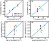 |
Fig. 2. Comparison of the inversion parameters and the simulation parameters. The colors represent the nine individual absorbing features. |
Based on this test, we conclude that our inversion can be used to reasonably infer the values of velocity, temperature, and density in the Hα-absorbing plasma structures. It is useful to fine-tune the inversion aided by tests based on the synthetic data for a precise inference of the physical parameters.
4. Application to real observations
4.1. Data
We used the Hα line spectral data of the 2020 July 30 observation of a small quiet region done with the Fast Imaging Solar Spectrograph (FISS, Chae et al. 2013) of the Goode Solar Telescope at Big Bear Solar Observatory. The observed region was scanned every 25 seconds for a duration of 83 minutes from 16:48:12 UT. The spatial resolution of the FISS data is limited by the sampling size of 0.16″, and is estimated to be about 0.32″. This dataset is the same as was used in the previous studies of transverse MHD waves (Kwak et al. 2023), a network jet (Lim et al. 2025), and the Doppler velocity oscillations in a rosette (Chae et al. 2025). We only analyzed one scanned dataset taken at 17:01:58 UT in detail. The spectral data were reduced following the procedures described by Chae et al. (2013). The wavelength was calibrated to ensure that the center of the FOV-averaged line profile has no Doppler shift. The Hα spectrum at every position was recorded from −5.0 to 4.7 Å at a sampling of 0.019 Å, which is fine enough to avoid degrading the spectral resolution of the FISS, which was estimated to be 0.045 Å. We applied the fitting to the spectral data from −2.5 to 2.5 Å. All the line profiles were normalized by I0, the continuum intensity averaged over the field of view, which is about the same as the continuum intensity at 6563 Å at the solar disk center.
4.2. Model fitting
Figure 3 shows the Hα monochromatic images constructed from the FISS observation of a small quiet-Sun region that is located near the disk center. The observed field of view includes a well-shaped network rosette that consists of the bright central region and the surrounding mottle (or fibril) region, in which a number of radially directed dark mottles occur. Outside the rosette are internetwork regions. The central region of the rosette displays elongated bright features that are identified at the Hα centerline, previously referred to as bright mottles (e.g., Bray 1969). These bright mottles are not cloud-like plasma structures, but simply represent brighter background Hα lights (Tsiropoula et al. 2012). We constructed the reference background intensity profile Iλ,ref by averaging a total of 51 200 observed intensity profiles taken from the whole field of view shown in Fig. 3.
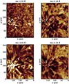 |
Fig. 3. Monochromatic images constructed at several wavelengths. The field of view is 32″ by 41″ sampled at 0.16″ in both directions. The four positions at which the model fit is examined are marked by symbols and numbers. |
Figure 4 illustrates the model fitting to the observed line profiles taken from Hα-absorbing plasma structures of different types. The profile in panel (a) is taken from the position in a mottle marked by (a) (see Fig. 3). In this case, the model fit produced a background intensity profile Iλ, 0 that is practically the same as the given Iλ,ref. The optical thickness profile τλ was modeled by three Gaussian components specified by the values of w, τb, vb, τc, vc, τr, and vr. The value of w has a physical meaning because it yields the estimate of T. The individual values of the other six model parameters are not physically meaningful, but the physical parameters derived from them, such as m, vM, vE, and vF, are physically meaningful. From the model fitting at this position, we obtained the estimated values and the statistical errors in the estimates T = (8.3 ± 0.1)×103 K, m = (4.5 ± 0.2)×10−5 g cm−2, vM = −7.9 ± 0.2 km s−1, vE = 12.1 ± 0.3 km s−1, and vF = −12.7 ± 0.3 km s−1.
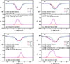 |
Fig. 4. Model fit to the Hα line profiles at the four positions (a to d) marked in Fig. 3. The line intensities are normalized by the continuum intensity at the disk center. |
The profile in panel (b) was taken from a position in an internetwork feature (see Fig. 3), called a Hα dark grain (Beckers 1964). This type of feature appears as a dark patch in the Hα blue wing, but is not visible in the centerline and the Hα red wing. Fig. 4b clearly shows that in this case, Iλ, 0 deviates much from Iλ,ref. Lee et al. (2000) indicated that Hα line profiles of this type often occur in dark grains and cannot be fit by the classical cloud model because of the red wing emission. The figure shows that our model successfully fits this type of line profile as well. The constructed Iλ, 0 matches the red wing of Iλ,obs well, but deviates strongly from Iλ,ref. With this constructed Iλ, 0, the observed profile Iλ,obs is fairly well modeled by a cloud model with an optical thickness practically of a single velocity component. In this case, we obtain T = (9.0 ± 0.2)×103 K, m = (4.8 ± 0.2)×10−5 g cm−2, vM = −16.9 ± 0.1 km s−1, vE = 17.8 ± 0.1 km s−1, and vF = −18.6 ± 0.1 km s−1.
The observed line profile Iλ,obs in panel (c) was taken from a faint Hα-absorbing plasma structure in the central region of the rosette. In this case, the constructed profile Iλ, 0 is also far from the profile Iλ,ref. Iλ,ref is found to be lower than Iλ,obs at the centerline and near the wings because it was obtained by averaging all the profiles inside the observed field of view. It is very encouraging that our model can construct an Iλ, 0 that is suitable for a faint Hα-absorbing feature inside the bright network center. In this specific case, the optical thickness profile was well modeled by a single-Gaussian velocity component. The determined parameters are T = (7.3 ± 1.2)×103 K, m = (2.3 ± 2.1)×10−5 g cm−2, vM = 18.2 ± 4.0 km s−1, vE = 19.0 ± 1.2 km s−1, and vF = 19.8 ± 1.2 km s−1.
Finally, the observed complex line profile in panel (d) was taken from a very dynamic feature, the Hα jet investigated by Lim et al. (2025). This line profile also can be reasonably well fit by our model, with three Gaussian components of different velocities. Because the feature is very dynamic, even the central velocity component had a velocity of −19.2 km s−1. From the model fitting of this line profile, we obtained the parameters T = (12.3 ± 0.2)×103 K, m = (31.0 ± 1.7)×10−5 g cm−2, vM = −26.5 ± 0.4 km s−1, vE = 32.0 ± 0.3 km s−1, and vF = −34.3 ± 0.2 km s−1. In this feature, we might have overestimated T because it is likely that the nonthermal speed ξ in a dynamic feature is higher than those of quiescent features. Our temperature estimate is higher than 10.0 × 10³ K, the value determined by Lim et al. (2025). We chose ξ = 8.0 km s−1, whereas Lim et al. (2025) independently estimated ξ at 10 km s−1 at this specific time.
In this section, we have specified the statistical errors in the determination of T, m, vM, vE, and vF. We conclude that they are usually negligibly small, which indicates that the fits are satisfactory enough.
4.3. Source function, temperature, and mass
Figure 5 presents the spatial distribution of the model parameters and physical parameters in the observed FOV. The map of S is not shown in the figure because S is less important to us than the other parameters. It suffices to specify that it has a mean of 0.15 and a standard deviation of 0.07 in the FOV. The map of τw indicates how much Hα-light absorption occurs in each region. Every Hα absorption structure seen in the −0.5 Å, +0.0 Å, and +0.50 Å images in Fig. 3 can be identified as a structure of τw enhancement in this Fig. 5. The map of T indicates that T varies from one structure to the next. Its mean over the FOV is 7.3 × 10³ K, and the standard deviation of its spatial fluctuation is 1.0 × 10³ K.
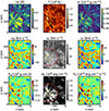 |
Fig. 5. Maps of the physical parameters wavelength-integrated optical thickness τw, temperature T, and column mass density m (upper panels), mass flux-associated velocity vM, kinetic energy-associated velocity vE, and kinetic energy flux-associated velocity vF (middle panels), mass flux FM, kinetic energy EK, and kinetic energy flux FK (lower panels). The central region of the network rosette is bounded by the yellow circle, and the mottle region is bounded by the yellow and red circles. |
We note that temperatures lower than 6.0 × 10³ K were obtained in some high-absorption regions, and temperatures higher than 12 × 103 were also obtained at a few plasma structures. It is particularly noteworthy that the jet at position (d) that was previously investigated by Lim et al. (2025) was significantly hotter than the mottles. This difference indicates the physical difference between the jet and the mottles, and it supports the proposed magnetic reconnection origin of the jet.
The mean of m over the FOV is found to be ⟨m⟩ = 2.7 × 10⁻⁵ g cm−2, and its standard deviation is σ(m) = 2.3 × 10⁻⁵ g cm−2. With the choice of H = 500 km, the mean mass density of the Hα-absorbing structures is estimated to be 5.4 × 10⁻¹³ g cm−3. In addition, the number distribution of m is very similar to the Poisson distribution. We regarded m at each location as a multiple of the unit column mass m0. When m/m0 follows a Poisson distribution, it is required that the mean of m/m0 is equal to the variance of m/m0, from which we obtained the estimate m0 = σ2(m)/⟨m⟩ = 2.0 × 10⁻⁵ g cm−2. The simple emerging picture is that a Hα absorption structure is the superposition of the unit absorption structures of the column mass m0. We find that ⟨m⟩/m0 = 1.4, which means that a 1.4 unit absorption structure exists on average along the vertical line at each location.
4.4. Doppler velocities
The method we employed for the velocity distribution allowed us to define three types of Doppler velocities at each point: vM, vE, and vF. The spatial distributions of these velocities over the FOV are shown in Fig. 5. The map of vM in Fig. 5 indicates that plasma structures in the FOV move at high speeds either upward or downward with a rough statistical balance between the two directions. This property is supported by the fact that the absolute value of ⟨vM⟩ = 0.7 km s−1 is much lower than the standard deviation σ(vM) = 8.5 km s−1. The typical speed of the moving structures is measured as ⟨|vM|⟩ = 6.8 km s−1. This value we obtained is higher than the corresponding values of mottles reported previously, ⟨|vM|⟩ = 3.6 − 3.9 km s−1 (Grossmann-Doerth & Von Uexküll 1971, 1973), and it is higher than those inferred in previous studies, ⟨|vM|⟩ ≃ 5.5 km s−1 (Tsiropoula et al. 1993) and 4.0 km s−1 (Tziotziou et al. 2003).
The difference in the measurement of vM between our results and previous results can partly be attributed to the difference in spatial resolution. Observations with a higher spatial resolution are less subject to the line-of-sight overlap of features that move at different speeds than observations with a lower spatial resolution. Pereira et al. (2013) illustrated the effect of the limb spicule superposition that arises from a low spatial resolution and low cadence on the measured properties of spicules and showed that previous measurements can be misleading. It is therefore not inconceivable that a similar error occurs in the Doppler velocity measurements of mottles.
The measurements of vE and vF are relevant to the energetics. This type of measurement is done here for the first time. A very important property is that vE and vF have higher speeds than vM. Over the FOV, we obtained ⟨vE⟩ = 14 km s−1 and ⟨|vF|⟩ = 12 km s−1. These values are much higher than ⟨|vM|⟩. This strongly suggests that vM alone cannot characterize the Doppler motion of Hα-absorbing plasma structures in relation to the kinetic energy. In other words, it is crucial to employ vE and vF to evaluate the kinetic energy and kinetic energy flux inferred from the Doppler motion properly.
Figure 6a presents the number distributions of vM, vE and vF in the mottle region. The histograms in this figure were constructed with the weighting number m/m0 at each position. In the mottle region, vM mostly ranges from −20 to 20 km s−1 with a mean of 1.3 km s−1 and a standard fluctuation of 8.5 km s−1, vE ranges from 5 to 25 km s−1, and vF ranges from −22 to 23 km s−1. The most important value is probably ⟨vE⟩ = 15 km s−1, which is slightly higher than the FOV average value of 14 km s−1.
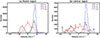 |
Fig. 6. (a) Histograms of vM, vE and vF in the mottle region. (b) Histograms of these parameters in the central region. |
Figure 6b presents the number distributions of vM, vE, and vF in the central region. Here, vM ranges from −29 to 25 km s−1 with a mean of 0.50 km s−1 and a standard fluctuation σ(vM) = 11 km s−1, vE ranges from 12 to 34 km s−1, and vF ranges from −35 to 25 km s−1. All of these characteristics are represented by the high value ⟨vE⟩ = 18 km s−1. The Doppler velocities in this region often reach 25 km s−1, which is a typical speed of rising motions in spicules (Beckers 1972). These high-velocity features in the central part might therefore be the disk counterparts of limb spicules, especially those emanating from the rosette centers.
These Hα-absorbing structures in the rosette center might be the same as the mottles in the surrounding mottle region, but they might appear to be different because of the difference in the magnetic field inclination. Structures in the central region might be moving along predominantly vertical fields, and mottles might be moving along inclined magnetic fields. When their velocity of motion along magnetic fields is the same, the observed Doppler velocities of the mottles are lower than those of the central region structures. Assuming the inclination is about 45 degrees, we multiplied the estimate ⟨vE⟩ = 15 km s−1 by the factor  to obtain 21 km s−1, which is even higher than ⟨vE⟩ = 18 km s−1 obtained in the central region and close to the typical speed of limb spicules. The fast-moving Hα-absorbing structures in the rosette center might therefore be a low-inclination version of conventional mottles, and these two types of Hα-absorbing structures might both represent the disk counterparts of limb spicules and mottles.
4.5. Mass flux
We obtained estimates of the mean mass flux and its standard fluctuation, ⟨FM⟩ = 0.2 × 101 g cm−1 s−1 and σ(FM) = 3.9 × 101 g cm−1 s−1. By dividing these values by H = 500 km, we obtained ⟨FM⟩/H = 0.4 × 10⁻⁷ g cm−2 s−1 and σ(FM)/H = 7.8 × 10⁻⁷ g cm−1 s−1. |⟨FM⟩|/H is smaller than σ(FM)/H by a factor of 20, which means that nearly all the rising material eventually falls back.
4.6. Kinetic energy and kinetic energy fluxes
Our results indicate that the upper chromosphere is a reservoir of kinetic energy. This type of nonthermal energy eventually dissipates into heat. We obtained ⟨EK⟩ = 5.6 × 10⁷ erg cm−2 and ⟨FK⟩= − 0.9 × 10¹³ erg cm−1 s−1 over the FOV.
If the kinetic energy is replenished at every Δt = 5 minutes, for example, which is the reported lifetime of visible spicules (Beckers 1972), we obtain an estimate of the kinetic energy flux as ⟨EK⟩/Δt = 1.9 × 10⁵ erg cm−2 s−1. This energy flux is on the same order of magnitude as the energy losses of 6 × 10⁵ erg cm−2 s−1 in the upper chromosphere and corona (Withbroe & Noyes 1977).
If the kinetic energy is contained in the vertical columns of H = 500 km height, we derive another estimate of the kinetic energy flux of ⟨FK⟩/H = −1.8 × 10⁵ erg cm−2 s−1. The negative sign here means that net kinetic energy was transported upward. Its absolute value is close to the ⟨EK⟩/Δt estimated above. It is interesting that two different estimates produce values of the kinetic energy flux that are comparable to the radiative loss within a factor of three.
Our estimate of the kinetic energy flux is much higher than previous estimates. Tsiropoula & Tziotziou (2004) reported 0.44 × 10⁵ erg cm−2 s−1 as the estimate of kinetic energy flux averaged over the Sun, and Al et al. (2004) reported 0.3 × 10⁵ erg cm−2 s−1 in the mottles. This discrepancy suggests that calculating the kinetic energy flux based on the cloud model parameters is not a trivial task. Our approach is based on the velocity distribution function and helps in this regard.
4.7. Hydrogen ionization and internal energy
Based on the estimates of ρ and T, we calculated the fraction of hydrogen ionization xH using a generalized Saha equation (Chae 2021), where the photoionization rate is to be given as an independent input. We adopted the photoionization rate of 7.0 × 10⁻³ s−1, which is suitable for the atmospheric height of 2200 km, as given in Chae (2021). As a result, we obtained the value of xH and plasma pressure p at every position, resulting in the estimates ⟨xH⟩ = 0.32 and σ(xH) = 0.01, ⟨p⟩ = 0.37 dyn cm−2, and σ(p) = 0.05 dyn cm−2.
As we determined T, xH, and m at every position, we determined the thermal kinetic energy Uth and the hydrogen ionization energy UH using the expressions
 (23)
(23)
 (24)
(24)
We estimated the column density of the internal energy at ⟨Uth⟩ = 2.6 × 10⁷ erg cm−2 and ⟨UH⟩ = 8.9 × 10⁷ erg cm−2. The ⟨EK⟩ = 5.6 × 10⁷ erg cm−2 estimated above is higher than ⟨Uth⟩ and lower than ⟨UH⟩. Despite these differences, ⟨EK⟩ and ⟨U⟩≡⟨Uth⟩+⟨UH⟩ are still comparable to each other within a factor of two.
The internal energy comprises the thermal kinetic energy and the ionization potential energy, and the ionization potential energy is much higher than the thermal kinetic energy. This suggests that the ionization of hydrogen is very important in the energetics of the Hα-absorbing plasma. The heat released by the dissipation of nonthermal kinetic energy is probably mostly used to ionize hydrogen atoms, which increases the potential ionization energy. Hydrogen ionization thus plays the role of a thermal reservoir that maintains the plasma temperature more or less constant despite the heating, as was observationally illustrated for a chromospheric jet by Lim et al. (2025).
5. Summary and discussion
It is crucial to determine the physical parameters of Hα-absorbing plasma structures to understand the magnetohydrodynamics and energetics of the upper chromosphere. We have proposed a new approach to determining their physical parameters from Hα spectral data. In this approach, the Hα spectral data were fit with a three-layer background plus a three-component cloud model we developed. The fit was realized with the technique of a constrained least-squares fit.
We used the model parameters we determined to construct the velocity distribution function, with which we calculated the temperature, mass, mass flux, kinetic energy, and kinetic energy flux. These parameters were used in turn to define three different types of Doppler velocities: the mass-flux-associated velocity vM, the kinetic-energy-associated velocity vE, and the kinetic-energy-flux-associated velocity vF. The mass density, pressure, and hydrogen ionization can also be estimated.
We used the three velocity components of the cloud to construct the velocity distribution function without attempting to differentiate among the three velocity components. This approach is particularly helpful when the three components are so close in the velocity space that they cannot be separated from one another. On the other hand, when the three components are clearly separable in the velocity space, the individual components might be used to infer the physical parameters of the individual cloud components that move at different velocities. This promising aspect of our spectral inversion model can be exploited in future works.
Our new approach was successful in inferring the physical parameters from the Hα line profiles in various types of Hα-absorption plasma structures in the observed quiet-Sun region. The new approach worked well for the mottles, for a jet in the network rosette, and for Hα grains in the internetwork regions. It also worked in faint absorption structures in the internetwork region and in the bright central region of the network rosette.
We found that high-speed Doppler velocities are often found in the Hα-absorbing plasma structures. In the central region of the rosette, a Doppler motion with speeds > 18 km s−1 is common, and in the mottle region, a Doppler motion with speeds > 15 km s−1 is common. The inclination effect is taken into account, and our analysis of the Doppler velocities therefore supports that high-speed motions > 20 km s−1 are prevalent in the central region and in the mottles. Thus, our results resolve the long-standing discrepancy in velocity measurements between mottles on the disk and spicules outside the limb. Furthermore, our results suggest that high-speed features in the center of the network rosette might also become the disk counterparts of some spicules.
The kinetic energy budget of the upper chromosphere is high enough for the radiative losses in the upper chromosphere and corona in the quiet Sun. Moreover, the estimated kinetic energy is comparable to the estimated internal energy within a factor of two, which suggests that an energy conversion between kinetic energy and internal energy might occur. These results support the hypothesis that the motion of plasmas in Hα-absorbing structures is important in heating the upper chromosphere and corona. This conclusion based on the on-disk spectrograph observations is very compatible with similar conclusion drawn from the high-resolution imaging observations of limb spicules (De Pontieu et al. 2007).
The inferred high-speed Doppler motions of Hα-absorbing plasma structures are in fact alternating upward and downward motions. This well-known property of mottle motions is also supported by our finding that the standard fluctuations in the mass flux and kinetic energy flux are far higher than the absolute values of the net mass flux and the net kinetic energy flux. The Doppler motions should therefore be interpreted as oscillations and waves and not as flows. This view is not at all new because the high-speed motions observed in limb spicules were previously interpreted as slow shock waves (Hollweg 1982; De Pontieu et al. 2004) or transverse MHD waves (De Pontieu et al. 2007). Following the same line of thought, efforts were made to detect oscillations and waves from disk observations of mottles and fibrils. In high-resolution imaging observations of mottles, Kuridze et al. (2012) detected a number of transverse oscillations with a median velocity amplitude of 8.0 km s−1 and a median period of 165 s. Kuridze et al. (2013) further investigated transverse oscillations in mottles, determined their phase speeds, and interpreted the observed oscillations as magnetohydrodynamic kink waves, for instance, with velocity amplitudes up to 12 km s−1 and phase speeds up to 100 km s−1.
On the other hand, Chae et al. (2025) investigated the characteristics of Doppler velocity oscillations in the rosette shown in Fig. 3 in detail by analyzing the time series of the model parameters. They found that the oscillations had total powers from 2 to 8 km2 s−2 ( corresponding to velocity amplitudes of 2 to 4 km s−1) and peak periods from 4 to 6 min in the central region, a total power from 5 to 20 km2 s−2 (corresponding to velocity amplitudes of 3 to 5 km s−1), and a peak period from 6 to 20 min in the mottle region. This study strongly supported the hypothesis that Doppler motions are in fact oscillations and waves, and the authors suggested that longitudinal waves and transverse waves exist together in mottles and other Hα-absorbing structures. Because Chae et al. (2025) used the model parameters determined from the multilayer spectral inversion (Chae et al. 2021) that did not incorporate the cloud model, the velocity amplitudes above might have been underestimated in comparison with the results obtained from the three-layer-plus-three-component cloud model inversion we developed.
Together with these previous studies of oscillations and waves, our result for the estimate of the kinetic energy budget appears to support the hypothesis that magnetohydrodynamic waves heat the upper atmosphere of the quiet Sun. Longitudinal (e.g., slow MHD waves) and transverse waves (e.g., kink waves) are apparently both important. Specifically, our finding of common occurrence of velocities > 15 km s−1 appears to be compatible with the analytical study of Chae & Lee (2023) on the Alfén wave connection between the chromosphere and the corona of the Sun and the observational findings of high-amplitude transverse waves from the high-resolution imaging of a quiet region (Chae et al. 2024).
Although the hypothesis above is accepted, it does not necessarily negate the importance of magnetic reconnection that ubiquitously occurs in the quiet Sun. Magnetic reconnection is a good mechanism for exciting slow MHD waves, as was theoretically conjectured (e.g, Sturrock 1999) and observationally supported (e.g, Yang et al. 2014). Spicules appear to originate from the site at which opposite-polarity magnetic flux appears around dominant-polarity magnetic field concentrations (Samanta et al. 2019). This observation might be interpreted as evidence that magnetic reconnection in the lower atmosphere drives waves that result in spicules. This scenario differs from the p-mode driving scenario, in which the leakage of the p-mode oscillations into the chromosphere along inclined magnetic fields drives slow shock waves that result in spicules (De Pontieu et al. 2004). In either case, MHD waves drive the spicules.
We conclude that MHD waves are probably crucial for the Hα-absorbing plasma structures in the upper chromosphere and for the heating of the upper chromosphere and corona. The outstanding problem then is to evaluate the relative importance between p-mode oscillations and ubiquitous small-scale magnetic reconnection in driving MHD waves in the upper atmosphere.
Acknowledgments
We appreciate the referee’s constructive comments. We are grateful to Jorrit Leenaarts for providing the simulation data, and to Ryunyoung Kwon and Soosang Kang for careful manuscript reading and suggestions. This research was supported by the National Research Foundation of Korea (RS-2023-00208117). K.-S. L. was supported by the National Research Foundation of Korea (RS-2025-23523356). E.-K.L. acknowledges support by the Korea Astronomy and Space Science Institute under the R & D program of the Korean government (MSIT; No. 2026-1-830-05). M.M. acknowledges the support of the Brain Pool program funded by the Ministry of Science and ICT through the National Research Foundation of Korea (RS-2024-00408396) and DFG grant WI 3211/8-2, project number 452856778. H.K. was supported by Basic Science Research Program through the National Research Foundation of Korea(NRF) funded by the Ministry of Education(RS-2024-00452856) BBSO operation is supported by US NSF AGS 2309939 grant and the New Jersey Institute of Technology. The GST operation is partly supported by the Korea Astronomy and Space Science Institute and the Seoul National University.
References
- Al, N., Bendlin, C., Hirzberger, J., Kneer, F., & Trujillo Bueno, J. 2004, A&A, 418, 1131 [NASA ADS] [CrossRef] [EDP Sciences] [Google Scholar]
- Bate, W., Jess, D. B., Nakariakov, V. M., et al. 2022, ApJ, 930, 129 [NASA ADS] [CrossRef] [Google Scholar]
- Beckers, J. M. 1964, Ph.D. Thesis, Sacramento Peak Observatory, Air Force Cambridge Research Laboratories, Mass., USA [Google Scholar]
- Beckers, J. M. 1968, Sol. Phys., 3, 367 [NASA ADS] [Google Scholar]
- Beckers, J. M. 1972, ARA&A, 10, 73 [NASA ADS] [CrossRef] [Google Scholar]
- Bray, R. J. 1969, Sol. Phys., 10, 63 [Google Scholar]
- Chae, J. 2014, ApJ, 780, 109 [Google Scholar]
- Chae, J. 2021, J. Astron. Space Sci., 38, 83 [Google Scholar]
- Chae, J., & Lee, K.-S. 2023, ApJ, 954, 45 [NASA ADS] [CrossRef] [Google Scholar]
- Chae, J.-C., Park, H.-M., & Park, Y.-D. 2007, J. Korean Astron. Soc., 40, 67 [NASA ADS] [CrossRef] [Google Scholar]
- Chae, J., Park, H.-M., Ahn, K., et al. 2013, Sol. Phys., 288, 1 [NASA ADS] [CrossRef] [Google Scholar]
- Chae, J., Yang, H., Park, H., et al. 2014, ApJ, 789, 108 [NASA ADS] [CrossRef] [Google Scholar]
- Chae, J., Madjarska, M. S., Kwak, H., & Cho, K. 2020, A&A, 640, A45 [NASA ADS] [CrossRef] [EDP Sciences] [Google Scholar]
- Chae, J., Cho, K., Kang, J., et al. 2021, J. Korean Astron. Soc., 54, 139 [Google Scholar]
- Chae, J., van Noort, M., Madjarska, M. S., et al. 2024, A&A, 687, A249 [NASA ADS] [CrossRef] [EDP Sciences] [Google Scholar]
- Chae, J., Lim, E.-K., Kang, J., Lee, K.-S., & Madjarska, M. S. 2025, A&A, 698, A259 [NASA ADS] [CrossRef] [EDP Sciences] [Google Scholar]
- De Pontieu, B., Erdélyi, R., & James, S. P. 2004, Nature, 430, 536 [Google Scholar]
- De Pontieu, B., McIntosh, S. W., Carlsson, M., et al. 2007, Science, 318, 1574 [Google Scholar]
- Foukal, P. 1971, Sol. Phys., 20, 298 [NASA ADS] [CrossRef] [Google Scholar]
- Grossmann-Doerth, U., & Von Uexküll, M. 1971, Sol. Phys., 20, 31 [Google Scholar]
- Grossmann-Doerth, U., & Von Uexküll, M. 1973, Sol. Phys., 28, 319 [Google Scholar]
- Hansteen, V. H., De Pontieu, B., Rouppe van der Voort, L., van Noort, M., & Carlsson, M. 2006, ApJ, 647, L73 [Google Scholar]
- Hansteen, V. H., Martinez-Sykora, J., Carlsson, M., et al. 2023, ApJ, 944, 131 [NASA ADS] [CrossRef] [Google Scholar]
- Hollweg, J. V. 1982, ApJ, 257, 345 [NASA ADS] [CrossRef] [Google Scholar]
- Judge, P. G., Kleint, L., Leenaarts, J., Sukhorukov, A. V., & Vial, J.-C. 2020, ApJ, 901, 32 [Google Scholar]
- Kuridze, D., Morton, R. J., Erdélyi, R., et al. 2012, ApJ, 750, 51 [NASA ADS] [CrossRef] [Google Scholar]
- Kuridze, D., Verth, G., Mathioudakis, M., et al. 2013, ApJ, 779, 82 [NASA ADS] [CrossRef] [Google Scholar]
- Kwak, H., Chae, J., Lim, E.-K., et al. 2023, ApJ, 958, 131 [NASA ADS] [CrossRef] [Google Scholar]
- Langangen, Ø., De Pontieu, B., Carlsson, M., et al. 2008, ApJ, 679, L167 [Google Scholar]
- Lee, C.-Y., Chae, J., & Wang, H. 2000, ApJ, 545, 1124 [Google Scholar]
- Leenaarts, J., Carlsson, M., & Rouppe van der Voort. L. 2012, ApJ, 749, 136 [NASA ADS] [CrossRef] [Google Scholar]
- Lim, E.-K., Chae, J., Cho, K., et al. 2025, ApJ, 981, 185 [Google Scholar]
- Pereira, T. M. D., De Pontieu, B., & Carlsson, M. 2012, ApJ, 759, 18 [Google Scholar]
- Pereira, T. M. D., De Pontieu, B., & Carlsson, M. 2013, ApJ, 764, 69 [Google Scholar]
- Pereira, T. M. D., Rouppe van der Voort, L., & Carlsson, M. 2016, ApJ, 824, 65 [Google Scholar]
- Rouppe van der Voort, L. H. M., De Pontieu, B., Hansteen, V. H., Carlsson, M., & van Noort, M. 2007, ApJ, 660, L169 [Google Scholar]
- Samanta, T., Tian, H., Yurchyshyn, V., et al. 2019, Science, 366, 890 [NASA ADS] [CrossRef] [Google Scholar]
- Sturrock, P. A. 1999, ApJ, 521, 451 [Google Scholar]
- Suematsu, Y., Wang, H., & Zirin, H. 1995, ApJ, 450, 411 [Google Scholar]
- Tsiropoula, G., & Schmieder, B. 1997, A&A, 324, 1183 [NASA ADS] [Google Scholar]
- Tsiropoula, G., & Tziotziou, K. 2004, A&A, 424, 279 [NASA ADS] [CrossRef] [EDP Sciences] [Google Scholar]
- Tsiropoula, G., Alissandrakis, C. E., & Schmieder, B. 1993, A&A, 271, 574 [NASA ADS] [Google Scholar]
- Tsiropoula, G., Tziotziou, K., Kontogiannis, I., et al. 2012, Space Sci. Rev., 169, 181 [Google Scholar]
- Tziotziou, K., Tsiropoula, G., & Mein, P. 2003, A&A, 402, 361 [NASA ADS] [CrossRef] [EDP Sciences] [Google Scholar]
- Vernazza, J. E., Avrett, E. H., & Loeser, R. 1981, ApJS, 45, 635 [Google Scholar]
- Withbroe, G. L., & Noyes, R. W. 1977, ARA&A, 15, 363 [Google Scholar]
- Yang, H., Chae, J., Lim, E.-K., et al. 2014, ApJ, 790, L4 [NASA ADS] [CrossRef] [Google Scholar]
All Figures
|
Fig. 1. Inversion model fit to a synthetic Hα line profile of an absorption feature. |
| In the text | |
|
Fig. 2. Comparison of the inversion parameters and the simulation parameters. The colors represent the nine individual absorbing features. |
| In the text | |
|
Fig. 3. Monochromatic images constructed at several wavelengths. The field of view is 32″ by 41″ sampled at 0.16″ in both directions. The four positions at which the model fit is examined are marked by symbols and numbers. |
| In the text | |
|
Fig. 4. Model fit to the Hα line profiles at the four positions (a to d) marked in Fig. 3. The line intensities are normalized by the continuum intensity at the disk center. |
| In the text | |
|
Fig. 5. Maps of the physical parameters wavelength-integrated optical thickness τw, temperature T, and column mass density m (upper panels), mass flux-associated velocity vM, kinetic energy-associated velocity vE, and kinetic energy flux-associated velocity vF (middle panels), mass flux FM, kinetic energy EK, and kinetic energy flux FK (lower panels). The central region of the network rosette is bounded by the yellow circle, and the mottle region is bounded by the yellow and red circles. |
| In the text | |
|
Fig. 6. (a) Histograms of vM, vE and vF in the mottle region. (b) Histograms of these parameters in the central region. |
| In the text | |
Current usage metrics show cumulative count of Article Views (full-text article views including HTML views, PDF and ePub downloads, according to the available data) and Abstracts Views on Vision4Press platform.
Data correspond to usage on the plateform after 2015. The current usage metrics is available 48-96 hours after online publication and is updated daily on week days.
Initial download of the metrics may take a while.