| Issue |
A&A
Volume 706, February 2026
|
|
|---|---|---|
| Article Number | A356 | |
| Number of page(s) | 8 | |
| Section | The Sun and the Heliosphere | |
| DOI | https://doi.org/10.1051/0004-6361/202556851 | |
| Published online | 19 February 2026 | |
Proton acceleration during the interaction of a coronal-mass-ejection-driven shock and a current sheet
1
Center for Space Plasma and Aeronomic Research (CSPAR), The University of Alabama in Huntsville Huntsville AL 35805, USA
2
Institut für Experimentelle und Angewandte Physik, Christian-Albrechts-Universität zu Kiel 24118 Kiel, Germany
3
Department of Space Science, The University of Alabama in Huntsville Huntsville AL 35805, USA
4
Institut für Physik und Astronomie, Universität Potsdam Potsdam, Germany
★ Corresponding author: This email address is being protected from spambots. You need JavaScript enabled to view it.
Received:
13
August
2025
Accepted:
19
December
2025
Abstract
Conext. Shock geometry plays a critical role in the acceleration of energetic particles. To isolate its effect, it is essential to study particle behavior under different shock geometries while maintaining comparable shock properties such as strength, speed, and turbulence conditions within a continuous period of time.
Aims. We aim to study the physical process of the interaction between an interplanetary shock and a current sheet, and compare the dynamic behavior of energetic protons under different shock geometries separated by the current sheet using the Electron-Proton Telescope on board the Solar Orbiter (SolO) on 14 March 2023.
Methods. We applied a partial-variance-increment (PVI) method to detect the magnetic structure in the upstream region of the shock. We reconstructed the proton pitch-angle distribution (PAD) in the solar wind frame to analyze the particle dynamics. We calculated the first-order flux anisotropy in the solar-wind frame of reference.
Results. We find that the differential flux of 60 keV–2 MeV protons is enhanced by 2.5 times from the current sheet to the shock. During the quasi-parallel shock interval, the first-order flux anisotropy in the solar-wind frame is consistent with diffusive shock acceleration. Nevertheless, the flux anisotropy exhibits a bipolar shape during the quasi-perpendicular shock interval. The coexistence of positive and negative flux anisotropy suggests that the magnetic field is wandering around the shock and connected to the shock surface with different acceleration efficiencies. That the flux anisotropy peaks at a transition energy may indicate that it is influenced by the current sheet. The transition energy is greater during the quasi-perpendicular interval, implying more efficient proton acceleration.
Conclusions. We suggest that the current sheet is an important ingredient that affects the local shock geometry and, thus, the particle acceleration efficiency and flux anisotropy. This effect can accumulate as the shock propagates outward from the Sun and should be taken into account when interpreting particle spectral profiles at greater distances.
Key words: Sun: corona / Sun: coronal mass ejections (CMEs) / solar wind
© The Authors 2026
 Open Access article, published by EDP Sciences, under the terms of the Creative Commons Attribution License (https://creativecommons.org/licenses/by/4.0), which permits unrestricted use, distribution, and reproduction in any medium, provided the original work is properly cited.
This article is published in open access under the Subscribe to Open model. This email address is being protected from spambots. You need JavaScript enabled to view it. to support open access publication.
1. Introduction
The interplanetary shock driven by the interplanetary part of coronal mass ejections (CME) is an important structure in association with energetic-storm-particle (ESP) events (Reames 2013; Desai & Giacalone 2016). It is commonly observed that the energetic particle flux starts to increase several hours before the shock. The flux enhancement exhibits an initial gradual rise followed by a rapid rise to the maximum to form a plateau around the shock (Lario et al. 2003; Giacalone 2012). This time–intensity profile is qualitatively consistent with theoretical predictions of diffusive shock acceleration (Axford et al. 1977; Bell 1978; Blandford & Eichler 1987; Zank et al. 2000; Li et al. 2003; Rice et al. 2003; Yang et al. 2018, 2019) or super-diffusive transport (Zimbardo & Perri 2013).
The CME-driven shock can extend to widespread longitudes and/or latitudes as it propagates outward (Gopalswamy et al. 2009; Lario et al. 2016). It may thus interact with the Parker spiral magnetic field with different orientations, leading to a shock geometry that varies as a function of shock surface position and propagation time (Zank et al. 2006; Giacalone 2017; Kong et al. 2017; Chen et al. 2022). The shock geometry refers to the shock normal angle, θBn, which is defined as the angle between the upstream magnetic field and shock normal. θBn is an important factor that influences the shock acceleration efficiency, which is physically relevant to the diffusion coefficient anisotropy that the perpendicular diffusion coefficient is much smaller than its parallel counterpart in the context of shock-driven acceleration processes (Jokipii 1987; Zank et al. 2004, 2006).
Solar-wind turbulence has been found to be intermittent (Marsch & Tu 1994; Kiyani et al. 2009; He et al. 2019; Zhu et al. 2020). Intermittency or coherent structures are ubiquitous in the solar wind. A portion of the coherent structure may be the border between adjacent flux tubes (Bruno et al. 2001; Borovsky 2008), while another type may be generated as a result of an inhomogeneous turbulence cascade (Sorriso-Valvo et al. 1999; Zhou et al. 2004). A representative type of coherent structure is a current sheet, a large number of which exhibit large-angle magnetic-field rotations (Li 2008). Numerical work (Qin & Li 2008) has demonstrated that flux tubes bounded by current sheets can lead to the strong scattering of particles in both parallel and perpendicular directions. This implies that current sheets play an important role in particle transport through the inner heliosphere. As a current sheet is swept by an interplanetary shock, the local shock geometry has a chance of changing between quasi-parallel and quasi-perpendicular on account of the magnetic-field rotation of the structure itself. The waiting time for current sheets is observed to be on the order of tens of minutes in the heliocentric distance from 1 to 3 au (Miao et al. 2011). Therefore, current sheets markedly reduce the spatial and temporal scales of shock geometry variation as compared to the gradual variation imposed by the Parker spiral magnetic field. It significantly complicates particle injection and acceleration as the shock travels outward.
Particle acceleration at a quasi-parallel shock appears to be mostly consistent with diffusive shock acceleration (Zank et al. 2000), which is achieved via particle scattering by the self-excited wave spectrum or pre-existing turbulence (Rice et al. 2003; Li et al. 2003). Nevertheless, particle acceleration at a quasi-perpendicular shock remains an outstanding problem, although shock-drift acceleration can play a role. Particle scattering that enables the first-order Fermi acceleration at a quasi-perpendicular shock is perhaps less efficient due to the lack of self-excited turbulence. Some mechanisms have been proposed to explain particle acceleration around a quasi-perpendicular shock. The first one is through the magnetic-field line wandering as the plasma is convected from upstream to downstream (Zank et al. 2006). To the best of our knowledge, there is no direct observational evidence of a field line wandering around and across quasi-perpendicular interplanetary shock based on single-spacecraft measurements. Another important mechanism that can facilitate the shock acceleration with arbitrary shock geometry is via dynamically interacting magnetic islands/flux ropes separated by current sheets. During the interaction of particles with magnetic islands, the particles can be accelerated by the magnetic-island contraction and the induced anti-reconnection electric field (Pritchett 2008; Oka et al. 2010) from dynamically merging multiple islands (Zank et al. 2014, 2015; le Roux et al. 2015, 2018; Hu et al. 2018; Chen et al. 2019; Farooki et al. 2024). Observations and numerical simulations have demonstrated that this mechanism indeed plays a role in local particle acceleration in the shock downstream region and during CME-heliospheric-current-sheet (HCS) interaction (Khabarova et al. 2016; Zhao et al. 2018; Adhikari et al. 2019; Zhao et al. 2019; Nakanotani et al. 2021, 2022a,b). Therefore, physical processes related to current sheets are important in particle acceleration. However, the influence of an individual current-sheet structure on the local shock geometry and particle acceleration has been discussed less.
The ion energy spectra near a CME-driven shock normally shows a spectral break on the order of 1 MeV. Observed spectra are often better characterized by a double power-law, rather than an exponential rollover (Mewaldt et al. 2005). A formation mechanism for the double power-law was first proposed by Zank et al. (2000), which invoked the escape of higher energy particles to explain the softening of high-energy spectra. It has also been suggested that a double power law is a consequence of event-integrated spectra (Tylka et al. 2001; Cohen et al. 2005; Zhao et al. 2016). The spectral break has a complex dependence on the shock geometry, diffusion coefficient, and turbulence anisotropy (Zank et al. 2000). For example, Zank et al. (2006) showed that the quasi-perpendicular shock requires a higher injection energy and typically yields a lower maximum particle energy. Li et al. (2005) suggested that the break energy corresponds to the maximum achievable energy being accelerated by a traveling shock.
Since the launch of SolO on February 10 2020, it has been taking routine measurements of the energetic particles’ flux with the energetic particle detector (EPD) suite (Rodríguez-Pacheco et al. 2020). It collects energetic particles with unprecedentedly high time and energy resolutions. This capability allowed us to study the dynamic behavior of energetic particles on smaller scales (Yang et al. 2023, 2024, 2025).
In this work, we focused on the acceleration of energetic particles during the interaction of a CME-driven shock with an individual upstream current sheet. This coherent structure separates regions of a shock for which the geometries are quasi-parallel or quasi-perpendicular. This observation provides a good opportunity to directly compare the energy spectra under different shock geometries at a continuous time and investigate how the coherent structure affects the particle acceleration efficiency, flux anisotropy, and spectral indices.
2. Data and method
We used magnetic-field measurements from the magnetometer (MAG) (Horbury et al. 2020) on board the SolO. The proton moment data are from the proton and alpha particle sensor, an element of the solar wind analyser suite (Owen et al. 2020). We used the particle flux measurements from the electron proton telescope (EPT), which is dedicated to electron measurements in the energy range from ∼30 to ∼500 keV and ions from ∼50 keV to ∼5 MeV. It is one of the four sensors of the energetic particle detector (EPD) suite (Rodríguez-Pacheco et al. 2020). The EPT has two double-ended telescopes: the sunward and anti-sunward telescopes pointing toward and away from the Sun, in line with the nominal Parker spiral; the other pair pointing northward and southward out of the ecliptic plane. Each telescope has a circular field of view with a half width of 15° (Wimmer-Schweingruber et al. 2021). The cadence of EPT is 1 s, which is the highest time resolution to date for ion measurements in the corresponding energy range.
3. Observations
The ESP event was observed on 14 March 2023 at a heliocentric distance of R ∼ 0.6 au (Figure 1). A CME-driven shock crosses SolO at 01:08:28.600, where the magnetic field magnitude, |B|, solar wind speed, V, proton number density, n, and proton temperature, T increase dramatically. The shock parameters are listed in Table 1. The shock normal was calculated by the mixed-mode coplanarity method (Paschmann & Daly 1998; Zhao et al. 2021) and is almost aligned with the radial direction as indicated by the normal vector n in radial-tangential-normal (RTN) coordinates. The shock speed, Vsh, is about 719 km/s. The angle between the upstream mean magnetic field and shock normal, θBn, is ∼99°, implying the shock geometry is quasi-perpendicular. The magnetic compression ratio, rB, is 2.33, and the density compression ratio, r, is 2.25.
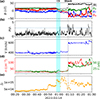 |
Fig. 1. Overview of ESP event observed by SolO on 14 March 2023. (a) Magnetic-field amplitude, |B|, and magnetic-field components in RTN coordinates. (b) PVI time series with τ = 60 s. (c) Solar-wind proton bulk speed,V. (d) Proton number density, n, and proton temperature, T. (e) Omni-directional proton differential flux, Jp, for particles with energies between 60 keV and 2 MeV in the solar-wind frame. The unit of Jp is /(cm2⋅s⋅sr⋅keV). The cyan shaded area indicates a current-sheet structure with prominent BN reversal. The vertical dashed line denotes the time of shock passage. |
Shock parameters.
The partial variance of increments (PVI) is a measure of the roughness of a magnetic field, B(t), which is closely related to the presence of coherent structures (Frisch 1995; Greco et al. 2009; Bruno & Carbone 2013; Matthaeus et al. 2015; Greco et al. 2018). The PVI time series is defined as
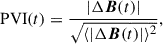 (1)
(1)
where ΔB(t) = B(t + τ)−B(t), τ is a chosen lag, and ⟨⋯⟩ denotes the time average of a trailing sample. A value of PVI(t) > 3 is a good indicator of the presence and location of a coherent structure. As shown in Figure 1(b), most PVI(t) > 3 values are present around the shock and its downstream region. There is only one PVI > 3 signal occurring in the upstream region at around 01:01:00. This large PVI value corresponds to a current sheet (CS) (Phan et al. 2006; Gosling & Szabo 2008; Phan et al. 2009; Mistry et al. 2015, 2017; Phan et al. 2022), as indicated by the cyan shaded area in Fig. 1. This CS structure shows a prominent BN reversal, an asymmetric |B| depression, and a local T enhancement (Fig. 1(a)–(d)). Fig. 1(e) shows the omni-directional proton differential flux, Jp, summed over an energy (E) range between 60 keV and 2 MeV. Jp presents three increases from upstream toward the shock. The first increase is at around 00:50. We note that there is no obvious magnetic-fluctuation-amplitude enhancement at this time. It is interesting to note that something appears to be accelerating them locally, especially given the smooth plasma and magnetic-field profiles. The second one is at around 00:58 when SolO encounters the CS and |B| starts to reduce. The Jp reaches its maximum between the CS and shock and forms a local dip around the shock. Hence, the CS has an impact on the local Jp variation. On average, the Jp between the CS and shock is 7.5 times greater than before the first increase and 2.5 times greater than after the first increase.
4. Properties of the current sheet
We first study the nature of the CS and the variation of the field and plasma properties associated with the CS. We converted the time series of the magnetic field and velocity in RTN coordinates to the hybrid minimum variance LMN coordinates (Gosling & Phan 2013), as shown in Fig. 2(b–c). The estimated LMN direction vectors are eL = [–0.37, –0.21, –0.91], eM = [–0.74, 0.65, 0.15], and eN = [–0.56, –0.72, 0.40]. The mean plasma velocity in RTN coordinates from 00:55:00–01:00:00 is V = [396.1, 1.2, –21.8] km/s. The mean plasma velocity in LMN coordinates is thus [–126.7 –296.7 –231.4] km/s. This suggests that the spacecraft mainly crosses the CS along the M and N directions.
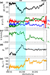 |
Fig. 2. Overview of field and plasma properties around current sheet. (a) Magnetic-field magnitude |B|. (b) Magnetic-field components in hybrid minimum variance LMN coordinates. (c) Ion velocity in L direction VL. (d) Plasma beta β. (e) Deflection angle of B from the shock-normal direction, θBn. |
Figure 2(a) shows that |B| is nearly constant before the CS. It gradually decreases to 8 nT, which is about a 60% reduction. Contemporaneously, BL changes direction, while BM remains at the average level (Fig. 2(b)). Nevertheless, |B| does not fully recover on the right side of the CS, but rather gradually increases from 01:00:30 to 01:08:28 when SolO encounters the shock. Fig. 2(c) shows that the VL component maintains an average level of -125 km/s until the center of the CS. It starts to decrease by about 60 km/s after the SolO crosses the plateau in BL. When |B| reaches the minimum, βp increases to a value as high as 2 due to the enhancement of Tp (Fig. 2(d)).
It is interesting to note that the magnetic-field rotation associated with this CS changes the angle between the magnetic field and the estimated shock-normal direction, θBn, from quasi-parallel to quasi-perpendicular (Fig. 2(e)). The magnetic-field direction is nearly constant until the |B| starts to increase after 01:00:30. θBn changes from ∼30° to ∼90° in around one minute. Between 01:00:30 and 01:08:00, 70% of the time periods have θBn < 90°. In this time interval, all angles are greater than 60°. Considering the CS is seven minutes ahead of the shock, if we assume that the shock front is nearly constant over at least one turbulence correlation length, the CS causes a change in the shock geometry from quasi-parallel to quasi-perpendicular for this particular event. In the next section, we demonstrate that the shock geometry change affects the particle acceleration and flux anisotropy.
5. Particle behavior under different shock geometries
In this section, we compare the dynamical behavior of energetic particles under different shock geometries separated by the CS by virtue of the closeness of the CS to the shock. Fig. 3(c) shows the pitch-angle (PA) distribution of the proton differential flux, Jp. The Compton-Getting effect (Compton & Getting 1935; Gleeson & Axford 1968) was corrected by converting the particle velocity into the solar-wind frame, using the same method as Yang et al. (2020, 2023). From 00:50:00–00:58:40 and 01:03:50–01:07:50, the EPT detector covers a similar PA range. This allowed us to directly compare the particle dynamics under different shock geometries eliminating the pitch-angle effect. We calculated the first-order flux anisotropy, An, in the solar-wind frame according to
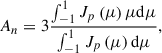 (2)
(2)
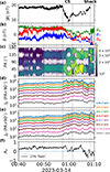 |
Fig. 3. (a) Magnetic-field magnitude |B|. (b) Magnetic-field components in RTN coordinates. (c) PA distribution of Jp for 276.7 keV protons in the solar-wind frame. (d) Total differential flux of protons with PA smaller than 90°. (e) Total differential flux of protons with PA greater than 90°. (f) First-order flux anisotropy for 276.7 keV protons in the solar-wind frame. The vertical dashed gray lines indicate the times of the current-sheet boundaries and the shock. |
where μ is the cosine of the PA (Dresing et al. 2014; Wei et al. 2024). Fig. 3(f) shows the flux-anisotropy variation for the 276.7 keV energetic protons.
Figure 3(d) shows the total Jp for protons whose PA range is smaller than 90°. In contrast, Fig. 3(e) shows the total Jp for protons with a PA greater than 90°. Before the CS, the intensity of energetic protons is constant overall, except for a slight increase for lower energy particles. Note that Jp is hardly affected by the PA coverage range (Fig. 4(c)). During this interval, the flux anisotropy is nearly constant, with an average value of 0.4. The Jp increases within the CS toward the shock. The increase is more significant for sunward energetic protons (PA > 90°), and a local isotropy distribution is realized in the CS at around 01:00. We suggest that this is due to the local enhancement of particle diffusion (Fig. 3(f)). In between the CS and the shock, the Jp decreases for PA< 90° protons, while the Jp is maintained at an average level for PA> 90° protons overall, although there are small-scale fluctuations. This leads to the dominance of sunward-propagating energetic particles and thus the presence of negative flux anisotropy. In this interval, interestingly, the flux anisotropy manifests as a bipolar shape (Fig. 3(f)).
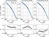 |
Fig. 4. Upper panels: Proton energy spectra, Jp(E), averaged over three time intervals and over the valid pitch-angle ranges. The blue and green circles indicate the observed spectra in the pitch angle ranges (30,70)° and (110,150)°, respectively. The corresponding solid lines are the pan-spectrum fitting results. The black dots mark the transition energy (spectral break) E0. Lower panels: First-order flux anisotropy, An, as a function of energy, E. |
Previous observational studies (Scholer et al. 1983; Sanderson et al. 1985; Wenzel et al. 1985; Kennel et al. 1986) have shown that An exhibits anisotropy away from the shock in the upstream region of interplanetary shock, either under quasi-parallel or quasi-perpendicular shock geometry. This phenomenon can be explained by a self-consistent theory for the excitation of upstream waves and the acceleration of ions (Lee 1983). Particularly, this theory predicts a near-constant moderate anisotropy at a value of ∼0.3 in the upstream region of quasi-parallel interplanetary shock, and the anisotropy value decreases with energy. This prediction is consistent with our observations before 00:58 (Fig. 3(f) and Fig. 4(d)), which is one justification of a quasi-parallel shock geometry interval.
The presence of both positive and negative An in the upstream region very close to the shock implies that both ends of the magnetic-field lines are connected to the shock surface. If the upstream magnetic-field lines are connected to the shock on one end and freely extend to the interplanetary space on the other end, a spacecraft will observe a positive An that indicates a bulk velocity of particles away from the shock. However, if a spacecraft detects a negative An in the upstream region, it may indicate that there is another particle source from the other end of the interplanetary magnetic field with greater intensity. In our event, we observe the negative An right before the shock passage, lasting less than two minutes. This indicates that the occurrence of negative An is a very local signature and probably results from a local physical process. In addition, the proximity to the shock implies that this negative An could originate from or be related to the shock. Hence, we suggest a possible explanation or scenario for the presence of negative An and the existence of both positive and negative values; that is, that the magnetic-field lines are connected to the shock on both ends. Such a configuration is consistent with a meandering magnetic field (Zank et al. 2006). The sign of An is determined by the relative acceleration efficiency at the two locations connected by the same magnetic -field lines. The generation of these extra sunward protons seems unlikely due to the first-order Fermi acceleration between the CS and the shock. This is because the CS is non-propagating in the solar-wind frame, specular reflection does not change the particle speed in the solar-wind frame, and the number of reflected particles cannot be greater than the number of incident particles coming from the shock.
Previous observations of sunward solar energetic particle events (Malandraki et al. 2002; Leske et al. 2012; Wei et al. 2024; Rodríguez-García et al. 2025; Ding et al. 2025) usually lasted several hours. The persistence of these sunward particles is more likely due to the acceleration at locations far away from the observer, in contrast to the very short period of negative An in our case. Hence, we infer that the occurrence of negative An (the sunward particles with greater intensity) may not come from a distant upstream region.
6. Upstream energy spectra and flux anisotropy at different energies
The upper panels of Fig. 4 show the average energy spectra in a symmetric pitch angle range with respect to 90° at three time intervals (00:50:00–00:58:00, 01:03:00–01:05:00, 01:06:00–01:07:30). The first interval corresponds to a quasi-parallel shock geometry, while the other two correspond to a quasi-perpendicular geometry. The PA ranges are (30,70)° and (110,150)°. All spectra exhibit a double-power-law shape with a smooth spectral break. We used a five-parameter pan-spectrum to fit all the observed spectra in the 50 keV-4 MeV energy range measured by EPT (Liu et al. 2020). The pan-spectrum reads as
![Mathematical equation: $$ \begin{aligned} J_p\left(E\right) = A\times \left(\frac{E}{E_0}\right)^{-\beta _1}\left[1+\left(\frac{E}{E_0}\right)^{-\alpha }\right]^{-\frac{\beta _1-\beta _2}{\alpha }}, \end{aligned} $$](/articles/aa/full_html/2026/02/aa56851-25/aa56851-25-eq3.gif) (3)
(3)
where β1 and β2 are the asymptotic spectral indices at lower and higher energies, respectively. E0 is the transition (break) energy, A is the amplitude, and α describes the spectrum width and sharpness around E0. The fit results are shown by the solid lines in Fig. 4. The fitting parameters are listed in Table 2. Note that the pitch angle ranges in these intervals are similar, and thus no pitch-angle effect is included.
Pan-spectrum fitting parameters of energy spectra.
The steady-state DSA with homogeneous background theoretically predicts an isotropic single-power-law spectrum with an index of β = 3r/(r − 1) in the reference frame of the shock. This leads to a positive anisotropy in the upstream solar-wind frame with a moderate value of 0.2–0.3 for tens to hundreds of keV protons (Sanderson et al. 1985). This anisotropy is more remarkable for low-energy particles. Since the shock compression ratio r = 2.25 (Table 1), the DSA-predicted phase-space density f(V)∼V−β ∼ V−5.4, and thus J(E)∼E−1.7. It can be seen that the β1 of all spectra are not greater than 1, which is slightly harder than the DSA prediction. As one approaches the shock, β1 increases for both spectra of PA ∈ (30, 70)° and PA ∈ (110, 150)°. The transition energy, E0, also increases from around 400 keV to 550 keV and 750 keV. The variations of spectral index and transition energy indicate a change of particle-acceleration efficiency, as well as the dominant acceleration mechanism (Decker & Vlahos 1986). Hence, for this particular event, the quasi-perpendicular shock geometry leads to a greater local acceleration efficiency than that of the quasi-parallel shock geometry due to the greater transition energy (Zank et al. 2007).
The bottom panels of Fig. 4 exhibit the An as a function of E in the solar wind frame. The first interval exhibits a moderate flux anisotropy. It decreases from ∼0.5 with increasing E for E < E0 and becomes roughly constant (A∼ 0.25) above it. The corresponding An in the shock reference frame is weaker (not shown here). The energy dependence of An is consistent with the DSA predictions (Krymskii 1977; Axford et al. 1977; Bell 1978; Lee 1983; Sanderson et al. 1985). For the second interval, An remains positive and peaks at E0. The differential fluxes increase in both directions as compared to the first interval, and the enhancement is greater for PA ∈ (110, 150)° protons. Conversely, An changes in the third interval; that is, it is entirely negative and reaches a minimum around the E0, suggestive of the dominance of energetic particles flowing anti-parallel to the mangetic field. The reversal of An is mainly on account of the decrease in the differential flux of PA ∈ (30, 70)° protons and is more distinct for protons of E < 1 MeV. Note that the flux anisotropy of lower-energy particles is reduced. We suggest that the CS can influence the proton-flux anisotropy in the quasi-perpendicular shock interval.
The An of 276.7 keV protons exhibits a bipolar-like anisotropy in between the CS and the shock (Fig. 3(f)). Specifically, the An is positive from 01:01:30–01:05:00 and negative from 01:06:00–01:07:30. These time ranges correspond to the second and third intervals in Fig. 4, respectively. Fig. 4(e–f) shows that the An for the second interval is positive in the energy range of 60 keV–5 MeV, while the third interval is negative in the same energy range. This indicates that the bipolar-like flux anisotropy in the time series exists for a wide energy range.
7. Summary and conclusion
In this work, we investigated the energetic proton dynamics upstream of a CME-driven shock that is interacting with an individual CS. The measurements were made by the four telescopes of the EPD/EPT instrument with unprecedentedly high time and energy resolutions. The CS is present seven-minutes upstream of the shock and shows a magnetic-field depression. The current sheet rotates the magnetic-field direction by 60° and results in θBn, changing the character of the shock from quasi-parallel to quasi-perpendicular. The Jp of 60 keV< E< 2 MeV protons is enhanced after crossing the CS and peaks in between the CS and the shock, while it reaches a local minimum around the shock passage time.
The CSs are able to modify the local shock geometry either along the shock surface or as the shock propagates outward. The variation of the shock geometry will affect particle acceleration. In our event, SolO first detects a quasi-parallel shock geometry and then enters a quasi-perpendicular region after crossing the CS. The Jp is nearly constant during the quasi-parallel interval. The An maintains a moderate level and the energy-dependence of An is qualitatively and partially quantitatively consistent with the DSA prediction. This also certifies that this interval corresponds to a quasi-parallel shock geometry, which is feasible for DSA. The An during the quasi-perpendicular interval is more complicated. Although the θBn is generally smaller than 90°, the An exhibit a bipolar shape. We suggest that it forms as a result of the magnetic-field connectivity and the interaction of the shock with the CS. The co-existence of positive and negative An implies that the SolO detects field lines with both directions connected to the shock. This can be achieved via the magnetic-field-line wandering, a mechanism favoring DSA around a quasi-perpendicular shock (Zank et al. 2006). The change of the An indicates that the SolO is magnetically connected to the shock surface with different acceleration efficiency. However, the energy dependence of An is inconsistent with the DSA prediction, which implies that the observed An may be affected by the CS as well. The CS increases the local particle diffusion particularly for lower energy particles. This makes the lower energy protons more isotropic.
Guo et al. (2010) studied the particle acceleration around a shock in the presence of a sinusoidal magnetic field by numerically solving the Parker transport equation. In their numerical results, if the connection points move toward each other, the magnetic field will trap and preferentially accelerate particles to high energies. Our observation is similar to this scenario based on two aspects. On one hand, the shock propagates outward, and thus the intersection points of the magnetic field with the shock surface will also gradually approach each other. On the other hand, the transition energy is greater during the quasi-perpendicular interval, indicating a more efficient particle acceleration in this region.
Previous work (Jebaraj et al. 2024) found that a quasi-parallel shock can become quasi-perpendicular locally on account of extended precursor whistler wave patches. For the first time, our work has provided evidence that an upstream current sheet is able to change the local shock geometry, which will affect the particle acceleration and flux anisotropy. We possibly provide the first evidence that magnetic-field-line wandering exists around a quasi-perpendicular shock based on the flux anisotropy. Our work highlights the importance of shock-structure interaction affecting the particle acceleration and flux anisotropy.
Acknowledgments
We acknowledge the partial support of the NSF award 2442628, NASA awards 80NSSC20K1783, 80NSSC23K0415, NSF EPSCoR RII-Track-1 Cooperative Agreement OIA-1655280. A.S. is partially supported by NASA FINESST award 80NSSC24K1867. Part of this work was supported by the German Deutsche Forschungsgemeinschaft, DFG project number Ts 17/2–1. L.Y. is partially supported by DFG under grant HE 9270/1-1.
References
- Adhikari, L., Khabarova, O., Zank, G. P., & Zhao, L. L. 2019, ApJ, 873, 72 [Google Scholar]
- Axford, W. I., Leer, E., & Skadron, G. 1977, Int. Cosmic Ray Conf., 11, 132 [Google Scholar]
- Bell, A. R. 1978, MNRAS, 182, 147 [Google Scholar]
- Blandford, R., & Eichler, D. 1987, Phys. Rep., 154, 1 [Google Scholar]
- Borovsky, J. E. 2008, J. Geophys. Res. (Space Phys.), 113, A08110 [NASA ADS] [Google Scholar]
- Bruno, R., & Carbone, V. 2013, Liv. Rev. Sol. Phys., 10, 2 [Google Scholar]
- Bruno, R., Carbone, V., Veltri, P., Pietropaolo, E., & Bavassano, B. 2001, Planet. Space Sci., 49, 1201 [Google Scholar]
- Chen, Y., Hu, Q., & le Roux, J. A. 2019, ApJ, 881, 58 [Google Scholar]
- Chen, X., Giacalone, J., & Guo, F. 2022, ApJ, 941, 23 [NASA ADS] [CrossRef] [Google Scholar]
- Cohen, C. M. S., Stone, E. C., Mewaldt, R. A., et al. 2005, J. Geophys. Res. (Space Phys.), 110, A09S16 [Google Scholar]
- Compton, A. H., & Getting, I. A. 1935, Phys. Rev., 47, 817 [NASA ADS] [CrossRef] [Google Scholar]
- Decker, R. B., & Vlahos, L. 1986, J. Geophys. Res., 91, 13349 [Google Scholar]
- Desai, M., & Giacalone, J. 2016, Liv. Rev. Sol. Phys., 13, 3 [NASA ADS] [CrossRef] [Google Scholar]
- Ding, Z., Wimmer-Schweingruber, R. F., Chen, Y., et al. 2025, A&A, 701, A123 [NASA ADS] [CrossRef] [EDP Sciences] [Google Scholar]
- Dresing, N., Gómez-Herrero, R., Heber, B., et al. 2014, A&A, 567, A27 [NASA ADS] [CrossRef] [EDP Sciences] [Google Scholar]
- Farooki, H., Noh, S. J., Lee, J., et al. 2024, ApJS, 271, 42 [Google Scholar]
- Frisch, U. 1995, Turbulence. The legacy of A. N. Kolmogorov [Google Scholar]
- Giacalone, J. 2012, ApJ, 761, 28 [NASA ADS] [CrossRef] [Google Scholar]
- Giacalone, J. 2017, ApJ, 848, 123 [NASA ADS] [CrossRef] [Google Scholar]
- Gleeson, L. J., & Axford, W. I. 1968, Ap&SS, 2, 431 [NASA ADS] [CrossRef] [Google Scholar]
- Gopalswamy, N., Yashiro, S., Michalek, G., et al. 2009, Earth Moon Planets, 104, 295 [NASA ADS] [CrossRef] [Google Scholar]
- Gosling, J. T., & Phan, T. D. 2013, ApJ, 763, L39 [Google Scholar]
- Gosling, J. T., & Szabo, A. 2008, J. Geophys. Res. (Space Phys.), 113, A10103 [NASA ADS] [CrossRef] [Google Scholar]
- Greco, A., Matthaeus, W. H., Servidio, S., Chuychai, P., & Dmitruk, P. 2009, ApJ, 691, L111 [Google Scholar]
- Greco, A., Matthaeus, W. H., Perri, S., et al. 2018, Space Sci. Rev., 214, 1 [NASA ADS] [CrossRef] [Google Scholar]
- Guo, F., Jokipii, J. R., & Kota, J. 2010, ApJ, 725, 128 [Google Scholar]
- He, J., Wang, Y., & Sorriso-Valvo, L. 2019, ApJ, 873, 80 [Google Scholar]
- Horbury, T. S., O’Brien, H., Carrasco Blazquez, I., et al. 2020, A&A, 642, A9 [NASA ADS] [CrossRef] [EDP Sciences] [Google Scholar]
- Hu, Q., Zheng, J., Chen, Y., le Roux, J., & Zhao, L. 2018, ApJS, 239, 12 [Google Scholar]
- Jebaraj, I. C., Agapitov, O., Krasnoselskikh, V., et al. 2024, ApJ, 968, L8 [NASA ADS] [CrossRef] [Google Scholar]
- Jokipii, J. R. 1987, ApJ, 313, 842 [NASA ADS] [CrossRef] [Google Scholar]
- Kennel, C. F., Coroniti, F. V., Scarf, F. L., et al. 1986, J. Geophys. Res., 91, 11917 [CrossRef] [Google Scholar]
- Khabarova, O. V., Zank, G. P., Li, G., et al. 2016, ApJ, 827, 122 [Google Scholar]
- Kiyani, K. H., Chapman, S. C., Khotyaintsev, Y. V., Dunlop, M. W., & Sahraoui, F. 2009, Phys. Rev. Lett., 103, 075006 [NASA ADS] [CrossRef] [Google Scholar]
- Kong, X., Guo, F., Giacalone, J., Li, H., & Chen, Y. 2017, ApJ, 851, 38 [Google Scholar]
- Krymskii, G. F. 1977, Akademiia Nauk SSSR Doklady, 234, 1306 [NASA ADS] [Google Scholar]
- Lario, D., Ho, G. C., Decker, R. B., et al. 2003, Am. Inst. Phys. Conf. Ser., 679, 640 [Google Scholar]
- Lario, D., Kwon, R. Y., Vourlidas, A., et al. 2016, ApJ, 819, 72 [NASA ADS] [CrossRef] [Google Scholar]
- le Roux, J. A., Zank, G. P., Webb, G. M., & Khabarova, O. 2015, ApJ, 801, 112 [Google Scholar]
- le Roux, J. A., Zank, G. P., & Khabarova, O. V. 2018, ApJ, 864, 158 [Google Scholar]
- Lee, M. A. 1983, J. Geophys. Res., 88, 6109 [NASA ADS] [CrossRef] [Google Scholar]
- Leske, R. A., Cohen, C. M. S., Mewaldt, R. A., et al. 2012, Sol. Phys., 281, 301 [NASA ADS] [CrossRef] [Google Scholar]
- Li, G. 2008, ApJ, 672, L65 [NASA ADS] [CrossRef] [Google Scholar]
- Li, G., Zank, G. P., & Rice, W. K. M. 2003, J. Geophys. Res. (Space Phys.), 108, 1082 [Google Scholar]
- Li, G., Zank, G. P., & Rice, W. K. M. 2005, J. Geophys. Res. (Space Phys.), 110, A06104 [Google Scholar]
- Liu, Z., Wang, L., Wimmer-Schweingruber, R. F., Krucker, S., & Mason, G. M. 2020, J. Geophys. Res. (Space Phys.), 125, e28702 [Google Scholar]
- Malandraki, O. E., Sarris, E. T., Lanzerotti, L. J., et al. 2002, J. Atmos. Sol.-Terr. Phys., 64, 517 [Google Scholar]
- Marsch, E., & Tu, C. Y. 1994, Ann. Geophys., 12, 1127 [NASA ADS] [CrossRef] [Google Scholar]
- Matthaeus, W. H., Wan, M., Servidio, S., et al. 2015, Philos. Trans. Royal Soc. A: Math. Phys. Eng. Sci., 373, 20140154 [Google Scholar]
- Mewaldt, R. A., Cohen, C. M. S., Labrador, A. W., et al. 2005, J. Geophys. Res. (Space Phys.), 110, A09S18 [Google Scholar]
- Miao, B., Peng, B., & Li, G. 2011, Ann. Geophys., 29, 237 [Google Scholar]
- Mistry, R., Eastwood, J. P., Phan, T. D., & Hietala, H. 2015, Geophys. Res. Lett., 42, 513 [Google Scholar]
- Mistry, R., Eastwood, J. P., Phan, T. D., & Hietala, H. 2017, J. Geophys. Res. (Space Phys.), 122, 5895 [NASA ADS] [CrossRef] [Google Scholar]
- Nakanotani, M., Zank, G. P., & Zhao, L. L. 2021, ApJ, 922, 219 [NASA ADS] [CrossRef] [Google Scholar]
- Nakanotani, M., Zank, G. P., & Zhao, L. 2022a, Front. Astron. Space Sci., 9, 954040 [Google Scholar]
- Nakanotani, M., Zank, G. P., & Zhao, L. L. 2022b, ApJ, 926, 109 [NASA ADS] [CrossRef] [Google Scholar]
- Oka, M., Phan, T.-D., Krucker, S., Fujimoto, M., & Shinohara, I. 2010, ApJ, 714, 915 [Google Scholar]
- Owen, C. J., Bruno, R., Livi, S., et al. 2020, A&A, 642, A16 [EDP Sciences] [Google Scholar]
- Paschmann, G., & Daly, P. W. 1998, ISSI Scientific Reports Series, 1 [Google Scholar]
- Phan, T. D., Gosling, J. T., Davis, M. S., et al. 2006, Nature, 439, 175 [Google Scholar]
- Phan, T. D., Gosling, J. T., & Davis, M. S. 2009, Geophys. Res. Lett., 36, L09108 [Google Scholar]
- Phan, T. D., Verniero, J. L., Larson, D., et al. 2022, Geophys. Res. Lett., 49, e96986 [NASA ADS] [CrossRef] [Google Scholar]
- Pritchett, P. L. 2008, J. Geophys. Res. (Space Phys.), 113, A06210 [Google Scholar]
- Qin, G., & Li, G. 2008, ApJ, 682, L129 [Google Scholar]
- Reames, D. V. 2013, Space Sci. Rev., 175, 53 [CrossRef] [Google Scholar]
- Rice, W. K. M., Zank, G. P., & Li, G. 2003, J. Geophys. Res. (Space Phys.), 108, 1369 [Google Scholar]
- Rodríguez-García, L., Gómez-Herrero, R., Dresing, N., et al. 2025, A&A, 694, A64 [NASA ADS] [CrossRef] [EDP Sciences] [Google Scholar]
- Rodríguez-Pacheco, J., Wimmer-Schweingruber, R. F., Mason, G. M., et al. 2020, A&A, 642, A7 [Google Scholar]
- Sanderson, T. R., Reinhard, R., van Nes, P., & Wenzel, K. P. 1985, J. Geophys. Res., 90, 19 [NASA ADS] [CrossRef] [Google Scholar]
- Scholer, M., Ipavich, F. M., Gloeckler, G., & Hovestadt, D. 1983, J. Geophys. Res., 88, 1977 [Google Scholar]
- Sorriso-Valvo, L., Carbone, V., Veltri, P., Consolini, G., & Bruno, R. 1999, Geophys. Res. Lett., 26, 1801 [NASA ADS] [CrossRef] [Google Scholar]
- Tylka, A. J., Cohen, C. M. S., Dietrich, W. F., et al. 2001, ApJ, 558, L59 [Google Scholar]
- Wei, W., Lee, C. O., Dresing, N., et al. 2024, ApJ, 973, L52 [NASA ADS] [CrossRef] [Google Scholar]
- Wenzel, K.-P., Reinhard, R., Sanderson, T. R., & Sarris, E. T. 1985, J. Geophys. Res., 90, 12 [Google Scholar]
- Wimmer-Schweingruber, R. F., Janitzek, N. P., Pacheco, D., et al. 2021, A&A, 656, A22 [NASA ADS] [CrossRef] [EDP Sciences] [Google Scholar]
- Yang, L., Wang, L., Li, G., et al. 2018, ApJ, 853, 89 [NASA ADS] [CrossRef] [Google Scholar]
- Yang, L., Wang, L., Li, G., et al. 2019, ApJ, 875, 104 [NASA ADS] [CrossRef] [Google Scholar]
- Yang, L., Berger, L., Wimmer-Schweingruber, R. F., et al. 2020, ApJ, 888, L22 [NASA ADS] [CrossRef] [Google Scholar]
- Yang, L., Heidrich-Meisner, V., Berger, L., et al. 2023, A&A, 673, A73 [NASA ADS] [CrossRef] [EDP Sciences] [Google Scholar]
- Yang, L., Heidrich-Meisner, V., Wang, W., et al. 2024, A&A, 686, A132 [NASA ADS] [CrossRef] [EDP Sciences] [Google Scholar]
- Yang, L., Li, X. Y., Heidrich-Meisner, V., et al. 2025, A&A, 695, A270 [NASA ADS] [CrossRef] [EDP Sciences] [Google Scholar]
- Zank, G. P., Rice, W. K. M., & Wu, C. C. 2000, J. Geophys. Res., 105, 25079 [NASA ADS] [CrossRef] [Google Scholar]
- Zank, G. P., Li, G., Florinski, V., et al. 2004, J. Geophys. Res. (Space Phys.), 109, A04107 [Google Scholar]
- Zank, G. P., Li, G., Florinski, V., et al. 2006, J. Geophys. Res. (Space Phys.), 111, A06108 [CrossRef] [Google Scholar]
- Zank, G. P., Li, G., & Verkhoglyadova, O. 2007, Space Sci. Rev., 130, 255 [Google Scholar]
- Zank, G. P., le Roux, J. A., Webb, G. M., Dosch, A., & Khabarova, O. 2014, ApJ, 797, 28 [Google Scholar]
- Zank, G. P., Hunana, P., Mostafavi, P., et al. 2015, ApJ, 814, 137 [Google Scholar]
- Zhao, L., Zhang, M., & Rassoul, H. K. 2016, ApJ, 821, 62 [Google Scholar]
- Zhao, L. L., Zank, G. P., Khabarova, O., et al. 2018, ApJ, 864, L34 [NASA ADS] [CrossRef] [Google Scholar]
- Zhao, L. L., Zank, G. P., Hu, Q., et al. 2019, ApJ, 886, 144 [Google Scholar]
- Zhao, L. L., Zank, G. P., He, J. S., et al. 2021, A&A, 656, A3 [NASA ADS] [CrossRef] [EDP Sciences] [Google Scholar]
- Zhou, Y., Matthaeus, W. H., & Dmitruk, P. 2004, Rev. Mod. Phys., 76, 1015 [NASA ADS] [CrossRef] [Google Scholar]
- Zhu, X., He, J., Wang, Y., & Sorriso-Valvo, L. 2020, ApJ, 893, 124 [Google Scholar]
- Zimbardo, G., & Perri, S. 2013, ApJ, 778, 35 [CrossRef] [Google Scholar]
All Tables
All Figures
|
Fig. 1. Overview of ESP event observed by SolO on 14 March 2023. (a) Magnetic-field amplitude, |B|, and magnetic-field components in RTN coordinates. (b) PVI time series with τ = 60 s. (c) Solar-wind proton bulk speed,V. (d) Proton number density, n, and proton temperature, T. (e) Omni-directional proton differential flux, Jp, for particles with energies between 60 keV and 2 MeV in the solar-wind frame. The unit of Jp is /(cm2⋅s⋅sr⋅keV). The cyan shaded area indicates a current-sheet structure with prominent BN reversal. The vertical dashed line denotes the time of shock passage. |
| In the text | |
|
Fig. 2. Overview of field and plasma properties around current sheet. (a) Magnetic-field magnitude |B|. (b) Magnetic-field components in hybrid minimum variance LMN coordinates. (c) Ion velocity in L direction VL. (d) Plasma beta β. (e) Deflection angle of B from the shock-normal direction, θBn. |
| In the text | |
|
Fig. 3. (a) Magnetic-field magnitude |B|. (b) Magnetic-field components in RTN coordinates. (c) PA distribution of Jp for 276.7 keV protons in the solar-wind frame. (d) Total differential flux of protons with PA smaller than 90°. (e) Total differential flux of protons with PA greater than 90°. (f) First-order flux anisotropy for 276.7 keV protons in the solar-wind frame. The vertical dashed gray lines indicate the times of the current-sheet boundaries and the shock. |
| In the text | |
|
Fig. 4. Upper panels: Proton energy spectra, Jp(E), averaged over three time intervals and over the valid pitch-angle ranges. The blue and green circles indicate the observed spectra in the pitch angle ranges (30,70)° and (110,150)°, respectively. The corresponding solid lines are the pan-spectrum fitting results. The black dots mark the transition energy (spectral break) E0. Lower panels: First-order flux anisotropy, An, as a function of energy, E. |
| In the text | |
Current usage metrics show cumulative count of Article Views (full-text article views including HTML views, PDF and ePub downloads, according to the available data) and Abstracts Views on Vision4Press platform.
Data correspond to usage on the plateform after 2015. The current usage metrics is available 48-96 hours after online publication and is updated daily on week days.
Initial download of the metrics may take a while.