| Issue |
A&A
Volume 706, February 2026
|
|
|---|---|---|
| Article Number | A347 | |
| Number of page(s) | 20 | |
| Section | Extragalactic astronomy | |
| DOI | https://doi.org/10.1051/0004-6361/202556999 | |
| Published online | 23 February 2026 | |
The redshifts from 122 bands: Comparative redshift forecast for low-resolution spectra from SPHEREx and the 7-Dimensional Sky Survey (7DS)
1
Astronomy Program, Department of Physics and Astronomy, Seoul National University 1, Gwanak-ro Gwanak-gu Seoul 08826, Republic of Korea
2
Korea Astronomy and Space Science Institute (KASI) 776, Daedeok-daero Yuseong-gu Daejeon, Republic of Korea
3
SNU Astronomy Research Center, Seoul National University Seoul 08826, Republic of Korea
4
Department of Earth, Environmental & Space Sciences, Chungnam National University 99 Daehak-ro Yuseong-gu Daejeon, Republic of Korea
5
Australian Astronomical Optics – Macquarie University 105 Delhi Road North Ryde NSW 2113, Australia
6
Department of Astronomy and Atmospheric Sciences, Kyungpook National University 80, Daehak-ro Buk-gu Daegu, Republic of Korea
7
Department of Astronomy, Yonsei University, 50 Yonsei-ro Seodaemun-gu Seoul 03722, Republic of Korea
8
California Institute of Technology 1200 E California Blvd Pasadena CA 91125, USA
9
IPAC, California Institute of Technology, 1200 E California Blvd, 91125 Pasadena, USA, California Institute of Technology 1200 E California Blvd Pasadena CA 91125, USA
10
Department of Earth Sciences, Pusan National University Busan 46241, Republic of Korea
11
School of Liberal Studies, Sejong University, 209 Neungdong-ro Gwangjin-Gu Seoul 05006, Republic of Korea
12
Department of Physics and Astronomy, Sejong University, 209 Neungdong-ro Gwangjin-Gu Seoul 05006, Republic of Korea
13
Institut d’Astrophysique de Paris, UMR 7095, CNRS, Sorbonne Université 98 bis boulevard Arago F-75014 Paris, France
★ Corresponding authors: This email address is being protected from spambots. You need JavaScript enabled to view it.
, This email address is being protected from spambots. You need JavaScript enabled to view it.
Received:
27
August
2025
Accepted:
21
December
2025
Abstract
The recently initiated SPHEREx and 7DS surveys will deliver low-resolution spectra (R ∼ 20 − 130) for hundreds of millions of galaxies over the optical to near-infrared range (0.4 − 5.0 μm), covering a wide sky area without sample selection. These unique datasets will improve redshift estimation and provide a rich redshift catalog for the community. In this study, we forecast the performance of photometric redshift estimations using simulated SPHEREx and 7DS data. Four widely used template-fitting approaches and two machine-learning (ML) methods are used to derive photometric redshifts from low-resolution spectrophotometric data. We measured redshifts using mock catalogs based on the GAMA and COSMOS galaxy samples and achieved high precision for bright (13 < i < 18) galaxies, with σNMAD ≲ 0.005, bias ≲0.005, and a catastrophic failure rate ≲0.005 for all methods employed. We find that the combined SPHEREx + 7DS dataset significantly improves redshift estimation compared to using either the SPHEREx or 7DS datasets alone, highlighting the synergy between the two surveys. Moreover, we compare the redshift estimation performance across magnitude ranges for the different methods and examine the probability distribution functions (PDFs) produced by the template-fitting approaches. As a result, we identify some factors that can affect the redshift measurements, for example, treatments on dust extinction or inclusion of flux uncertainty in the ML model. We also show that the PDFs are relatively well calibrated, although the confidence intervals are generally underestimated, particularly for bright galaxies in the template-fitting methods. This study demonstrates the strong potential of SPHEREx and 7DS to deliver improved redshift measurements from low-resolution spectrophotometric data, underscoring the scientific value of jointly utilizing both datasets.
Key words: galaxies: distances and redshifts / galaxies: general / cosmology: observations / infrared: galaxies
© The Authors 2026
 Open Access article, published by EDP Sciences, under the terms of the Creative Commons Attribution License (https://creativecommons.org/licenses/by/4.0), which permits unrestricted use, distribution, and reproduction in any medium, provided the original work is properly cited.
This article is published in open access under the Subscribe to Open model. This email address is being protected from spambots. You need JavaScript enabled to view it. to support open access publication.
1. Introduction
The redshift of a galaxy is one of the fundamental quantities we can measure through observations. It is the central quantity for measuring the distance to a galaxy and understanding the 3D structure of the Universe (e.g., Dawson et al. 2016; DESI Collaboration 2016; Reid et al. 2016; Ross et al. 2020). Moreover, the distances obtained from the redshifts scale bulk properties such as luminosity and mass, and even correlate with the cosmic epochs of the galaxies.
Spectroscopic observations can measure redshifts robustly as they can resolve the spectral features such as stellar continua or emission lines of the galaxies (Kurtz & Mink 1998; Cappellari 2017; Kim et al. 2025a). However, spectroscopic observations are biased toward the high signal-to-noise targets (e.g., bright galaxies with strong emission lines). Furthermore, many spectrographs employ slits (e.g., Hook et al. 2004) or fibers (e.g., Uomoto et al. 1999; Gunn et al. 2006) that limit the observable number of targets and necessitate the preselection of target galaxies (e.g., Prakash et al. 2015; Comparat et al. 2016; Hahn et al. 2023; Sohn et al. 2023). These observations are generally more costly and are limited to a small number of targets compared to imaging observations. There are slitless spectrographs (Euclid Collaboration: Scaramella et al. 2022; Wang et al. 2022), but they can be affected by blending of spectra in a crowded field.
Alternatively, photometric redshift (photo-z) estimations from multiband photometry can provide redshifts of galaxies without spectroscopic data (Baum 1962; Koo 1985; Arnouts et al. 1999; Weaver et al. 2022; Feder et al. 2024; Shuntov et al. 2025). Photo-z values have played an important role in the research of galaxy evolution and cosmology (see Zheng & Zhang 2012; Salvato et al. 2019; Newman & Gruen 2022 for reviews). Photo-z values are advantageous for studying galaxy populations as they can offer redshifts for all detected galaxies without preselection, although they are generally less precise than spectroscopic redshifts due to the low spectral resolution (R = λ/Δλ) of the photometric data.
This aspect is particularly beneficial for statistical studies of large galaxy samples. For example, when investigating the redshift dependence of galaxy properties with redshift bins sufficiently larger than the typical error of photo-z estimations, the error of the photo-z becomes insignificant compared to other sources of uncertainty (Newman & Gruen 2022). Furthermore, using statistical measures such as the mean of photo-z values reduces the importance of individual uncertainties, thereby improving the precision in science cases that rely on the statistical properties of large samples. Therefore, many studies that probe large-scale structures (e.g., Boris et al. 2007; Sánchez et al. 2011; Scoville et al. 2013; Ko et al. 2024; Euclid Collaboration: Laigle et al. 2025), galaxy clustering (e.g., Durret et al. 2011; Carnero et al. 2012; Castignani & Benoist 2016; Crocce et al. 2016; Zhou et al. 2021), weak and strong lensing (e.g., Treu 2010; Mandelbaum 2018; Cha et al. 2025), and cosmology (e.g., Blake & Bridle 2005; Seo et al. 2012; Masters et al. 2015; Hildebrandt et al. 2017) utilized photo-z values.
We can estimate the photo-z values of the galaxies with two primary approaches. The first is a template-fitting method that exploits the prior knowledge of the spectral energy distributions (SEDs) of galaxies (Arnouts et al. 1999; Brammer et al. 2008; Stickley et al. 2016; Lee & Chary 2020; Brammer 2021; Laur et al. 2022). This method compares the observed SED from multiband photometry with the template SEDs and finds the best-fit template and redshift.
The second approach allows us to infer the relation between the photometric data and the true redshifts using machine learning (ML) techniques (Collister & Lahav 2004; Beck et al. 2016; Laur et al. 2022; Kim et al. 2025b; Pathi et al. 2025). These ML-based methods try to find the relation between the multiband data and the true redshifts. They generally train the relation using a training sample with known redshifts. In the literature, many ML techniques are utilized to measure photo-z values, for example, neural networks (Collister & Lahav 2004; Pathi et al. 2025), random forests (RFs; e.g., Carrasco Kind & Brunner 2013; Kim et al. 2025b), convolutional neural networks (e.g., Henghes et al. 2022), and Gaussian processes (e.g., Gomes et al. 2018; Almosallam et al. 2016).
Although these efforts enhance the photo-z precision and accuracy above 1/R, the intrinsically low R of broadband data limits photo-z precision and accuracy for the given depth. This limits the applicability of photo-z values in cosmological and galactic studies. For example, scatter in the photo-z values can obscure the large-scale structures of galaxies, while biases and catastrophic failures can introduce biases in clustering analyses (Newman & Gruen 2022).
The low-resolution spectral surveys utilizing medium- to narrowband filters can yield improved photo-z values through denser spectral sampling compared to broadband surveys. Wolf et al. (2003) pioneered medium-band surveys with the Classifying Objects by Medium-Band Observations in 17 Filters (COMBO-17) survey. They showed a redshift accuracy of σ ≈ 0.03 for galaxies with R magnitude ≲24. The Multiwavelength Survey by Yale-Chile (MUSYC; Taylor et al. 2009; Cardamone et al. 2010) used 18 optical medium bands and other ancillary data and yielded σ ∼ 0.008 for galaxies with R magnitude < 25.3. The Physics of the Accelerating Universe Survey (PAUS, Eriksen et al. 2019) utilized 40 narrowband filters covering the 4500 − 8500 Å wavelength range. They achieved σ/(1 + z) = 0.0037 for the galaxies with magnitudes down to i ∼ 22.5 and with upper 50% photo-z qualities. The Javalambre-Physics of the Accelerating Universe Astrophysical Survey (J-PAS, Benitez et al. 2014) plans to survey 8500 deg2 of northern sky with 54 narrowband filters by utilizing a wide-field telescope with multiple detectors.
The recently started the Spectro-Photometer for the History of the Universe, Epoch of Reionization, and Ices Explorer (SPHEREx; Doré et al. 2014, 2016, 2018; Crill et al. 2020; Bock et al. 2025) and 7DS (7-Dimensional Sky Survey; Kim et al. 2024) projects are planned to overcome the limitation from coarse spectral sampling of broadband surveys across a wide sky area. SPHEREx enhances sky coverage by combining wide-field optics and linear variable filters (LVFs). 7DS improves survey efficiency through simultaneous observations using multiple wide-field telescopes equipped with different medium-band filters. These surveys will offer low-resolution (R ∼ 20 − 130) spectra for all the objects in the field of view from the optical (7DS) to the NIR (SPHEREx) wavelength range (0.4 − 5 μm) in a wide sky area.
The large volume of low-resolution spectral data from SPHEREx and 7DS will enable more precise and accurate redshift measurements. The SPHEREx and 7DS data lie between spectroscopic and photometric surveys, making them valuable for both spectroscopic and photometric redshift measurements. In this study, as we use the methods that have been utilized to measure photo-z values mainly exploiting the continuum features, we refer to the redshifts we obtain as photo-z.
Some previous studies assessed the performance of photo-z estimation with the simulated galaxy catalog of SPHEREx and 7DS. Stickley et al. (2016) and Feder et al. (2024) tested the photo-z estimation performance from mock SPHEREx data using the SPHEREx in-house code for photo-z measurements. The photo-z values from Feder et al. (2024) showed σ ∼ 0.0025, b (bias) ∼ − 0.0001, and η (catastrophic failure rate) ∼0.02 for the brightest galaxies in the sample (16.5 < W1 < 18.5).
Ko et al. (2025) tested the photo-z estimation performance with mock 7DS data using EAZY (Brammer et al. 2008). They reported σ ∼ 0.003 − 0.007 and η ∼ 0.008 − 0.081 for galaxies with 19 ≤ m(λ = 625 nm) < 22. They also tested a combination of 7DS data with mock Pan-STARRS1 (Chambers et al. 2016), VIKING (Edge et al. 2013), and SPHEREx full-sky survey data. In these tests, they find significant enhancement in the performance, especially when combined with the SPHEREx full-sky survey, achieving σ = 0.003 − 0.006 and η = 0.000 − 0.004 for the same magnitude range.
These studies demonstrated the potential of SPHEREx and 7DS for providing precise photo-z values for a large number of galaxies. However, Feder et al. (2024) mainly evaluated photo-z performance using mock SPHEREx and g, r, z, W1, and W2 data with the SPHEREx in-house photo-z code. On the other hand, Ko et al. (2025) conducted a photo-z performance assessment for combined SPHEREx + 7DS data, but they tested the performance solely with EAZY (Brammer et al. 2008) and employed the survey parameters for both SPHEREx and 7DS before updates. Since each study utilized one photo-z code, it remains unclear whether the photo-z performance of SPHEREx and 7DS data are consistent across different photo-z estimation codes. Furthermore, the synergy between these surveys can improve the scientific outputs beyond the intended level of the survey design, but this aspect has not been fully addressed with different photo-z measuring strategies.
For this paper we evaluated the photo-z performance of SPHEREx and 7DS surveys by applying six different photo-z estimation methods to the simulated survey datasets. Our aim was to assess the potential and the synergy of these surveys for photo-z measurements. We also attempted to investigate the strengths and weaknesses of different methods for this unique data and to find more optimized settings for future studies.
In Section 2 we outline the SPHEREx and 7DS surveys and the procedure for generating SPHEREx and 7DS mock catalogs. We describe the methods for estimating photo-z values in Section 3. We present the results for the SPHEREx + 7DS, SPHEREx, and 7DS datasets in Section 4 with the comparison between the methods as a function of i band magnitude and true redshift. In Section 5 we discuss the photo-z performance of SPHEREx and 7DS data and the synergy between them. We also analyze the differences in the results from different methods. Then we summarize our results and conclude in Section 6. Throughout this paper, we use the AB magnitude system (Oke & Gunn 1983).
2. Data
In this section, we outline the survey instruments, survey plans, and their scientific potential. We also summarize the SED templates and survey data for generating a mock catalog. We then describe the procedure to construct mock SPHEREx and 7DS galaxy catalogs that we used for estimating photo-z performance of the surveys.
2.1. Instruments and surveys
Figure 1 shows the depths of different survey layers, along with some other established large surveys with similar wavelength ranges. The figure shows the different depths of the three layers of 7DS and the two layers of SPHEREx surveys with square and circular markers, respectively. All the depths plotted are 5σ point source depths. The current best estimate (CBE) depths of SPHEREx surveys are based on the SPHEREx public git repository1. We simulated the depths of 7DS assuming the same observational and environmental parameters we used for generating the mock 7DS catalog used in this study, which are detailed in Section 2.2.4 and Ko et al. (2025). Figure 1 also shows the survey depths of SDSS (York et al. 2000), Pan-STARRS 3π survey (Chambers et al. 2016), VHS2 (McMahon et al. 2013), and unWISE (Schlafly et al. 2019). We also summarize the depths and survey coverage of the SPHEREx surveys and 7DS in Table 1.
Summary of the SPHEREx and 7DS surveys.
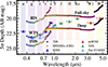 |
Fig. 1. 5σ point source detection limits of SPHEREx surveys and 7DS. The colored squares show the depths of the three layers of 7DS, with the RIS at the top, followed by the WTS and IMS layers. The circular markers show the depths of SPHEREx full-sky and deep surveys from the top. The blue, red, green, and pale blue triangles denote the 5σ point source depths of other popular optical and NIR imaging surveys (SDSS York et al. 2000, unWISE Schlafly et al. 2019, VHS McMahon et al. 2013, and Pan-STARRS Chambers et al. 2016). The shaded regions show the wavelength ranges of the plotted broadband filters as labeled at the top: u, g, r, i, z, Y, J, H, Ks, W1, and W2. |
2.1.1. SPHEREx
SPHEREx is a NASA Medium Explorer (MIDEX) mission that was successfully launched on March 11, 2025. It began its 25-month all-sky survey following completion of in-orbit checkout on May 1, 2025 (Doré et al. 2014; Crill et al. 2020; Bock et al. 2025). SPHEREx is conducting the first full-sky spectrophotometric survey in the NIR at wavelengths from 0.75 to 5.0 μm. Using a 20 cm wide-field telescope with a 3.5 × 11.3 deg2 instantaneous field of view, SPHEREx obtains spectra for every 6.15 × 6.15 arcsec2 pixel on the sky with resolving powers ranging from R = 35 to 130 (Korngut et al. 2018). SPHEREx utilizes LVFs, whose central wavelength varies linearly with position across the field of view. This unique technique allows SPHEREx to build a complete spectrum for each object of interest through successive exposures. Over its nominal two-year mission, SPHEREx will perform four all-sky surveys, capturing data across 102 spectral channels per sky position. To achieve Nyquist sampling of the spectral response, observations are offset by half a spectral channel between alternating survey passes.
SPHEREx’s survey strategy includes both a Full-Sky Survey and a Deep Survey. Each point along the ecliptic will be observed at least four times, with significantly higher redundancy in the deep survey fields near the north and south ecliptic poles (NEP and SEP), covering about 200 square degrees. Figure 1 shows the 5σ sensitivity per spectral channel, derived from the CBE. For the full-sky survey, the sensitivity reaches mAB ∼ 19.5 from 0.75 to 3.8 μm and mAB ∼ 19 − 17.5 from 3.8 to 5 μm. The deep survey regions achieve sensitivities that are approximately 2 magnitudes deeper than those of the full-sky survey.
Over its two-year primary mission, SPHEREx will provide a rich legacy catalog of over 1 billion galaxy spectra, over 100 million high-quality galaxy redshifts, tens of millions of stellar and ice absorption spectra, and thousands of quasar and asteroid spectra.3 Its scientific goals include mapping the 3D large-scale structure of the universe up to redshift z ≲ 2 to constrain inflationary physics, conducting intensity mapping of star formation history, and tracing the cosmic journey of water and biogenic molecules from the interstellar medium to planetary systems.
2.1.2. 7DT & 7DS
The 7-Dimensional Telescope (7DT, Kim et al. 2024) is an array of wide-field telescopes located in Chile’s El Sauce Observatory, consisting of 20 unit telescopes. Each unit telescope has a wide field of view of 1.33 × 0.89 deg2 with a 50 cm aperture and is equipped with a CMOS camera with a pixel scale of 0.5 arcsec.
7DT can observe the wide field of view using medium-band filters with 25 nm bandwidths and central wavelengths from 0.4 to 0.9 μm (R ∼ 30 − 60), with the central wavelengths between the adjacent filters separated by 12.5 nm. The central wavelength of the bluest medium-band filter is 400 nm, while it is 875 nm for the reddest one. The filters are named such as m400, where 400 is the three-digit number of the central wavelength in nm, while m stands for medium-band.
When each of the 20 7DT telescopes observes the same field using two medium-band filters with different central wavelengths, we can obtain a 40-wavelength spectral image over the entire field of view. This unique instrumental design will address various science cases, such as galaxy evolution (Kim et al. 2024; Lim et al. 2025), transient search (Paek et al. 2024; Khalouei et al. 2025), exoplanet atmospheres (Bae et al., in prep.), and cosmology.
Currently, 7DT uses 20 medium-band filters with each filter separated by 25 nm in central wavelengths (m400, m425, ..., m850, and m875). Throughout this paper, we assumed 7DT observations with these currently installed 20 filters. We expect that the future installation of an additional 20 filters would improve photo-z estimation accuracy (Ko et al. 2025).
7DS is an optical spectro-photometric survey conducted with 7DT (Kim et al. 2024), utilizing medium-band filters. 7DS consists of three layers with different survey depths and sky coverages to address a wide range of sciences: Reference Imaging Survey (RIS), Wide-field Time-domain Survey (WTS), and Intensive Monitoring Survey (IMS).
RIS will survey nearly the entire sky at Dec < 20 deg observable from the 7DT at the El Sauce Observatory, Chile (30.4725° S, 70.7631° W). The survey will capture the images with 300 seconds of on-source integration time per filter and tile. This survey will provide the widest view of the sky among the three survey layers and will be used as reference images for transient searches with target-of-opportunity observations. This survey is currently running, and we expect to complete the survey by next year.
WTS will visit each survey tile every ∼20 days with the same exposure time as the RIS per visit. This survey will cover ∼1600 deg2 of the southern sky. The survey field has not been decided, but WTS will explore long-term spectral variation of various objects such as active galactic nuclei (AGN). With 5 years of observations, this survey will have comparable depths to the SDSS survey (mAB ≲ 23, see Figure 1) with medium-band filters.
IMS will provide the deepest data among the 7DS layers. 7DT will visit the IMS survey tiles every observable night, providing the deepest data in the 7DS. The survey area will overlap with the SEP field of the SPHEREx deep survey to maximize the synergy between the two deep surveys.
2.2. Mock catalog
The mock catalogs of SPHEREx and 7DS data were from the simulated SEDs from Feder et al. (2024), who constructed mock spectra of the galaxies based on the COSMOS2020 (Weaver et al. 2022) and GAMA (Driver et al. 2022) multiband photometry data. Here we outline the galaxy SED templates and introduce the COSMOS and GAMA data used in this study. After that, we summarize the procedure to make mock catalogs used to test the performance of photo-z estimation.
Although we tried to faithfully simulate the real observations by considering several observational factors, the mock catalogs of SPHEREx and 7DS will have some differences compared to real data. The environmental and instrumental effects may be more complicated than our assumptions. In spite of that, our results can serve as a benchmark of the photo-z measurement performance of SPHEREx and 7DS data using different methods. Furthermore, the homogeneously processed mock data present an ideal sample for comparing the photo-z performance of different combinations of survey layers and different photo-z methods.
2.2.1. COSMOS and GAMA data
A large sample of galaxies with ground-truth redshifts is key to accomplishing a robust assessment of photo-z measurement performance. COSMOS data are ideal for this because they provide a deep and complete catalog of galaxies, representing the realistic distribution of magnitudes and redshifts of galaxies in the COSMOS field. They are based on the multiband photometry from COSMOS2020 (Weaver et al. 2022). The COSMOS2020 data consist of very deep (i ≲ 27) photometric data from 0.15 μm to 8 μm, covering ∼2 deg2 of the COSMOS field (Scoville et al. 2007; Weaver et al. 2022).
Among the COSMOS2020 galaxies, Feder et al. (2024) selected galaxies with i < 25 and at least one NIR band (i.e., UltraVISTA J or H band). They further selected galaxies with robust photo-z estimates that had consistent photo-z values from the two different photometry sets in Weaver et al. (2022). These selection criteria left 166 014 galaxies in the COSMOS field within the magnitude range of 18 < i < 25.
The COSMOS dataset provides a deep sample of galaxies well beyond the limiting magnitude of the SPHEREx and 7DS surveys (see Figure 1). However, it has a relatively low number of bright galaxies, which poses difficulties in assessing the photo-z performance for bright and low-redshift galaxies with i ≲ 20. As the SPHEREx full-sky, WTS, and RIS surveys cover a wide area with relatively shallow depths, measurements of photo-z performance for bright galaxies are important to assess their scientific potential.
In this regard, we also used the mock SEDs of GAMA galaxies (Driver et al. 2022), which were also constructed by Feder et al. (2024) from the multiband photometry included in the GAMA dataset. The GAMA sample contains 44 135 galaxies with i ≲ 18.5 across the four GAMA fields spanning ∼200deg2 in total (Feder et al. 2024).
Figure 2 shows the distribution of the GAMA and COSMOS samples in the i − ztrue parameter space. The GAMA and COSMOS samples show distinctive distributions in magnitudes and true redshifts.
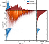 |
Fig. 2. Redshift and i magnitude distribution of GAMA and COSMOS galaxies used in this work. The GAMA data (bright blue) consists of brighter galaxies (i ≲ 18.5) with low redshifts (z ≲ 0.4) compared to COSMOS galaxies (maroon) with 18 ≲ i ≲ 25 and z ≲ 6. |
2.2.2. Brown+COSMOS templates
We used the Brown+COSMOS templates for template-fitting methods, which were compiled by Feder et al. (2024) and also used for constructing mock SEDs by fitting the observed multiband photometry data with these templates (See Section 2.2.3 and Feder et al. 2024 for more details). The authors combined template spectra from Brown et al. (2014) (Brown template) and Ilbert et al. (2009) (COSMOS template). The number of the compiled template set used in Feder et al. (2024) is 160, which consists of 129 Brown templates and 31 COSMOS templates.
Brown templates are a collection of local galaxy SEDs compiled and extended in Brown et al. (2014). This atlas of galaxies spans a broad range of galaxy types and environments. The authors combined optical and IR spectra and filled the wavelength range lacking observed spectra based on the SED model fitted to the photometric data using the MAGPHYS model (da Cunha et al. 2008). The resulting templates have wavelength coverage from 100 Å to 350 000 Å. They represent the broad population of local galaxies.
The COSMOS templates are a collection of templates from Polletta et al. (2007) and 12 additional model templates generated using the BC03 (Bruzual & Charlot 2003) stellar library for both starburst and passive elliptical galaxies. This template set has been widely used in COSMOS surveys (Ilbert et al. 2009, 2013; Laigle et al. 2016; Weaver et al. 2022). The COSMOS templates complement the Brown templates by including model-based templates and templates based on higher-redshift galaxies compared to Brown et al. (2014).
2.2.3. Mock SEDs
We adopted the mock SEDs constructed by Feder et al. (2024). We briefly describe the procedure used for making the mock SEDs used in this study, which is explained in Feder et al. (2024) in more detail. They generated mock SEDs using SED fitting to the observed COSMOS and GAMA multiband photometric data with Fitcat as in Stickley et al. (2016). Based on the photo-z value and the multiband photometric data, they modeled the SEDs with the Brown + COSMOS galaxy templates by finding the best-fit template, E(B − V), dust law, and stellar mass. Feder et al. (2024) report a median χr2 value of 2.2, with fewer than 1% of galaxies showing χr2 > 10. The relatively high χr2 values are partly driven by the limited template set, which especially may not fully capture complex PAH features, and by potentially underestimated photometric uncertainties in the COSMOS and GAMA photometric data. Despite these limitations, the errors in the mock SEDs are generally no larger than the expected photometric uncertainties of the SPHEREx and 7DS surveys, given the depths of the COSMOS and GAMA datasets. Although the IMS data reach similar depths, the mock SEDs from Feder et al. (2024) remain useful for providing realistic SEDs and enabling direct comparisons to shallower datasets. However, some template-driven biases or residuals may become detectable in the deepest IMS data.
Additionally, Feder et al. (2024) augmented emission lines to the fitted spectra. The strengths of Hα and [O II] were determined from the best-fit templates, and the observed scaling relations were then used to estimate the [N II] and Hβ line strengths, which were incorporated into the mock spectra. They also tested the injected emission-line strengths by comparing the line equivalent widths and luminosity functions with external measurements of COSMOS galaxies, and reported overall consistency.
2.2.4. Mock SPHEREx and 7DS data
We used the mock SEDs from Feder et al. (2024) to generate mock catalogs of SPHEREx and 7DS by simulating the observations. The SPHEREx catalog was generated using the SPHEREx Sky Simulator (Crill et al. 2025), a software tool designed to simulate the infrared observations of the SPHEREx mission. The simulator produces realistic infrared sky scenes using astrophysical models (such as zodiacal light and diffuse galactic light), the instrument’s unique spectrometer design and custom onboard detector readout, as well as the SPHEREx all-sky survey strategy. It incorporates realistic noise and systematic effects derived from up-to-date astrophysical measurements and prelaunch instrument characterization campaigns. The simulator can generate full spectral images per detector, matching the layout of the six detectors in one exposure, and produce photometric catalogs by performing forced photometry on the spectral image at preselected sky positions.
The SPHEREx Sky Simulator includes a QuickCatalog mode that bypasses full spectral image generation and directly simulates photometric measurements for given sources over the SPHEREx mission. We used this mode to generate simulated SPHEREx photometry for sources from the COSMOS2020 and GAMA catalogs. The inputs to the simulator are the mock SEDs and sky positions of the sources. Using the SPHEREx survey plan, the simulator identifies the pointings that observe each source, identifies detector positions, and computes the associated bandpasses. The transmission curves of the 102 bandpasses were generated from the wavelength response of the SPHEREx arrays by finding all pixels with the predefined central wavelengths. Simulated observations include realistic background emission, simulated point spread functions, and lab-measured noise realizations to enable accurate modeling of photometric uncertainties.
The generation of the 7DS mock data generally follows the procedure detailed in Ko et al. (2025). We first convolved the mock SEDs with the 7DS filter transmission curves. The 7DS filter transmission curves contain the information on the filter transmittance, quantum efficiency of the detector, telescope throughput, and sky transmission. For the detector and telescope information, we used instrumental information of the C3-61000 PRO camera4 and PlaneWave DeltaRho 500 (DR500) telescope5 (Kim et al. 2024). For sky transmission, we used the atmospheric model of Cerro Paranal site (Noll et al. 2012), with an airmass of 1.3 and a precipitable water vapor (PWV) of 2.5 mm, following Ko et al. (2025).
We calculated the error of the convolved fluxes by considering the Poisson noise, readout noise, and calibration error. We assumed the g2750 gain mode with a typical gain of 0.26e−/ADU. This gain mode was selected for the 7DS observations due to its lower readout noise (3.51e− for g0 vs. 1.46e− for g2750), which thus enables the detection of faint sources. We assumed 2″ seeing, a 2″-radius aperture for photometry, an observable night fraction of 70%, and a calibration error of 1% of the flux values. Using the simulated flux and the errors, we resampled the flux values with Gaussian distributions to mimic observed fluxes.
Although we followed the method for mock data generation, the process has some differences compared to that of Ko et al. (2025). We used the mock SEDs from Feder et al. (2024), but Ko et al. (2025) used the EL-COSMOS mock SEDs (Saito et al. 2020). Also, we applied updated survey strategies with different exposure times, filters, and detector gain settings. In particular, we assumed the current 20 medium-band filters for the 7DT filter set-up, while Ko et al. (2025) focused more on the 7DT performance using 40 medium-band filters.
We defined the deep and wide datasets considering the survey area and potential synergy between the survey layers of SPHEREx and 7DS. We focus on these two datasets in the following sections. We also present a 7DT RIS simulated sample as a reference for photo-z performance in comparison to other datasets.
The wide dataset contains the WTS from 7DS and the all-sky survey from the SPHEREx survey. This dataset includes all the COSMOS and GAMA galaxies, totaling ∼210 000 galaxies with 13 ≲ i ≲ 25 (cf. Figure 2). This sample will be used to test the surveys with wide sky coverages and relatively shallower depths.
The deep dataset consists of the IMS from 7DS and the deep survey from SPHEREx. As these two datasets cover relatively smaller sky areas intensively with more visits, this deep dataset is suitable for testing photo-z performance for fainter galaxies compared to the wide dataset. We randomly selected 1000 galaxies within the COSMOS dataset to make a representative sample of faint galaxies and define them as the deep sample.
Figure 3 shows the simulated mock SEDs from the SPHEREx and 7DS overplotted on the original SEDs from Feder et al. (2024). From the top to the bottom rows, the magnitudes of the sample galaxies become fainter. The simulated photometry reveals the differences in signal-to-noise ratio (S/N) between the wide and deep datasets. Specifically, continuum features such as the 4000 Å-break and the 1.6 μm bump are well captured in our mock data. The broad emission feature from PAH at 3.3 μm is also captured for the galaxies at low redshifts. Also, some strong line features such as Hα are captured in the data, as noted in previous research utilizing SPHEREx and 7DS mock data (Feder et al. 2024; Ko et al. 2025).
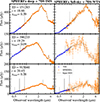 |
Fig. 3. Simulated SPHEREx and 7DS data used in this study. The gray plot shows the mock SED from Feder et al. (2024). The left column of the figure shows the simulated photometry of the deep dataset (SPHEREx deep + 7DS IMS) and the right column shows that of the wide dataset (SPHEREx full-sky + 7DS WTS), with the same example galaxies sorted in ascending i magnitudes. The blue markers show the mock datapoints from the 7DS, and the orange markers show the simulated SPHEREx datapoints. |
The mock catalogs contain some negative flux values resulting from random sampling of fluxes with their corresponding uncertainties. We treated these negative fluxes as nondetections and either excluded them or substituted them with dummy values during photo-z measurements (see Section 3). To remove the dependence of the training and test sets on the results of different ML-based methods, we defined the training and test sets in advance with FLAG_ML. The 20% of the galaxies in our sample were randomly selected as the test sample, and we assigned them FLAG_ML = 1.
The COSMOS galaxies with i ∼ 25 are much fainter than the survey limit of the wide dataset. Therefore, we used the COSMOS galaxies with 18 < i < 21 (N = 5065) for presenting the results from the wide dataset, as this magnitude range covers up to the median depth of the wide dataset (see Figure 1). We used fainter samples up to i = 23 when we presented and compared the results from the deep dataset. Though we did not use the whole sample of COSMOS galaxies for presenting results, we used it for training the models of ML-based methods. Note that when we show the results from ML-based methods, we present only the results from the test sample (FLAG_ML = 1).
3. Photo-z methods
We independently tested and optimized six methods to evaluate the performance for photo-z estimation of SPHEREx and 7DS mock data. Using these independent methods and configurations, our aim was to demonstrate that SPHEREx and 7DS data consistently yield accurate photo-z estimates. We also investigated some factors that influence the performance of photo-z estimation with these approaches. In this section, we outline the methods and settings used for measuring photo-z values. We tested four template-fitting methods and two ML-based methods.
3.1. SPHEREx in-house pipeline
SPHEREx in-house pipeline is a photometric redshift estimation code implemented in Stickley et al. (2016) and Feder et al. (2024). It is fundamentally similar to the widely used template-fitting code LePhare (Arnouts et al. 1999; Ilbert et al. 2006), but it has been reimplemented in C++ and adapted specifically for SPHEREx data, which involve hundreds of filters and demand high-throughput processing of large datasets.
The code performs χ2 minimization over a predefined grid of models using 160 templates, including those from the Brown and COSMOS libraries. The model grid spans E(B − V) values from 0 to 1 in steps of ΔE(B − V) = 0.1 for three dust extinction laws (Allen 1976; Prevot et al. 1984; Calzetti et al. 2000), and it covers redshifts from z = 0 to 3 in steps of Δz = 0.002. The grid size was determined after careful optimization. Although this redshift range limits the applicability of the models to sources at z ≤ 3, we did not extend the grid to higher redshifts because galaxies at z > 3 are expected to be faint and relatively rare in SPHEREx data. Flat priors were assumed over the parameter space and template set.
The code has thus far been tested only on simulated datasets. Priors and the template error function will be finalized and validated once SPHEREx data become available. We note that the expected value of the redshift probability distribution function (PDF) was adopted as the point estimate. Negative flux measurements were excluded from the fitting procedure.
3.2. EAZY
EAZY (Brammer et al. 2008) is a photo-z code written in the C language. This software is widely used to measure photo-z, along with its Python version that will be described below. This code estimates photo-z based on χ2 minimization. We can additionally impose a magnitude-redshift prior to exploit the trend of galaxies to be fainter at higher redshifts.
The size of the redshift grid is important for the precision of the photo-z measurements. When the grid is too fine, the calculation time becomes significantly longer. However, the size of the grid does not have a significant influence on the results when the S/N of the data is low. To balance between the precision of the measurements and the calculation time, we used magnitude-dependent redshift grids. We used a grid size of Z_STEP = 0.01 for i > 19 targets and Z_STEP = 0.001 for i ≤ 19 targets.
As noted above, we used the Brown + COSMOS templates from Feder et al. (2024) for SED fittings. However, among the Brown + COSMOS templates, the COSMOS templates do not have information for wavelengths shorter than 900 Å, which overlap with the 7DT wavelengths from z ≥ 3.44. The majority of the objects in the catalogs have lower redshifts, but some objects may be influenced by the incomplete short wavelength coverage of the templates in photo-z estimation. Therefore, we did not use the COSMOS templates, leaving 129 Brown templates in the photo-z estimation. We adjusted the corresponding configurations, such as the wavelength file, to the templates. While EAZY and eazy-py support multitemplate fitting – allowing the observed fluxes to be modeled as a linear combination of templates – this option substantially increases the computational cost. Given that the template set captures the main features of the SEDs observed in our sample, we opted for single-template fitting to reduce runtime without significant loss of accuracy.
The template error function was assumed to be constant at 5% for each template in all wavelengths (cf. Rudnick et al. 2001). When we use a nonzero template error function, the accuracy of the estimated photo-z improves as it smooths the resulting probability distribution of the photo-z posterior and increases the influence of the prior. This prevents the photo-z estimation from being a less plausible but global minimum in the posterior distribution. We also tested a photo-z performance using a template error function following Brammer et al. (2008) and found that the results remained similar. We therefore decided to adopt constant error functions in this study, as the error function constructed in this experiment is template- and sample-dependent and thus is not suitable for application to future real datasets, while also adding unnecessary complexity to the comparison. We used z_m2 as our point estimate from the resulting probability distribution function (PDF), which is calculated after marginalizing the magnitude-redshift prior.
We constructed a prior from the redshift-magnitude distribution of the galaxies for a certain band in the dataset, as the SPHEREx and 7DS have unique sets of bands. We used the m625 magnitude in the prior for 7DS and SPHEREx + 7DS datasets, as this band has the highest expected S/N among the SPHEREx and 7DS bands. When we measured photo-z values only with SPHEREx data, we used the 14th channel of detector 3 in SPHEREx, as this channel has the highest expected S/N.
We constructed the prior by fitting the magnitude-redshift distribution of the COSMOS dataset with the functional form from Equation (3) of Brammer et al. (2008). The COSMOS2020 (Weaver et al. 2022) data have an i-magnitude depth of ≲27 magnitude. This is much deeper than i ∼ 23 magnitude, which is the magnitude of the faintest galaxy that we present a photo-z in this study. Most of the bands used in COSMOS2020 have depths deeper than 23 magnitude, which makes the effect from the number of data points used in the SED construction of Feder et al. (2024) minimal for galaxies with i ≲ 23. Therefore, the COSMOS2020 photometric catalog and its corresponding mock SEDs built in Feder et al. (2024) are complete down to i ∼ 23 magnitude, and thus we used this sample to make a prior representative of the distribution of the galaxies within a specific volume in the real Universe. The resulting shape of the prior is very similar to the one illustrated in Figure 4 in Brammer et al. (2008).
3.3. eazy-py
The photo-z estimator eazy-py (Brammer 2021) is a Python implementation of EAZY, designed to reproduce the results of the original C version while offering improved flexibility in Python-based workflows. This software supports most of the functionalities provided by EAZY, including multitemplate fitting, the use of template error functions, and redshift priors. Owing to its reliability and integration within the broader Python ecosystem, eazy-py has become one of the most widely adopted photo-z estimation tools in the current era of the James Webb Space Telescope and ongoing medium- and narrowband imaging surveys (e.g., Lee et al. 2024).
Although EAZY and eazy-py share many properties, we used different redshift grids, template sets, template error functions, and priors, as we tuned the settings independently. We discuss the differences in the results in Section 5.3.
We estimated photo-z using the 160 Brown+COSMOS templates with single-template fitting. We used single-template fitting for the same reason as in the EAZY C version (see Section 3.2 for more details).
The redshift grid was defined with a step size of Z_STEP = 0.01, spanning the range from 0.002 to 5.8, chosen to encompass the redshift distribution of the sample. A constant template error of 0.01 was applied across all wavelengths. We also scaled the flux errors by a factor of 1.5 to improve the calibration of the redshift PDF, p(z), in separate validation tests using our deep dataset following the methods of Wittman et al. (2016) and Laur et al. (2022). Further discussion of this point is provided in Section 5.3.2.
As for redshift priors, we adopted the built-in Ks band prior (prior_K_TAO), derived from the Theoretical Astrophysical Observatory (TAO) lightcone simulation (Bernyk et al. 2016). For details on the prior-generation methodology, see Brammer et al. (2008, Section 2.5). This prior is linked to the 14th channel of SPHEREx band 3, which has a pivot wavelength of 2.2 μm, corresponding to the Ks band. For the 7DS-only sample, we instead applied the built-in R band prior (prior_R_zmax7), derived from the luminosity function of the semi-analytic model in De Lucia & Blaizot (2007), and linked it to the 7DT/m650 band.
Optimization was performed using the default non-negative least squares algorithm implemented in eazy-py (Lawson & Hanson 1974; Virtanen et al. 2020), and all negative flux values were excluded from the fitting. The final photo-z point estimate was taken to be the maximum a posteriori (MAP) redshift (zml), which is also the default output of eazy-py.
3.4. LePhare
The LePhare (Arnouts et al. 1999) is a photometric redshift estimation tool that utilizes the spectral energy distribution (SED) template-fitting method. In addition to redshifts, it can derive physical properties such as stellar mass, star formation rate, and dust content. As one of the longest-standing tools, LePhare has been widely adopted as a standard photometric redshift estimator in large surveys such as COSMOS (Weaver et al. 2022) and Canada-France-Hawaii Telescope Legacy Survey (CFHTLS; Ilbert et al. 2006; Coupon et al. 2009).
Among the parameters in LePhare, we set Z_STEP, which determines the step size of the redshift grid used for SED fitting, to 0.005. This value was chosen to balance accuracy and computational efficiency. We also tested Z_STEP = 0.002, but the redshift performance did not significantly improve even for bright GAMA galaxies. The best-fit redshifts were determined from the PDF computed with the χ2 minimization on a redshift grid, with parabolic interpolation applied to refine the grid beyond the resolution set by Z_STEP. No specific prior was applied, and neither dust extinction nor dust emission was considered, as these effects were already incorporated into the SED templates. Nondetections, which correspond to upper limits, can be handled in two ways: either excluded from the fitting (with −99 values), or used as upper-limit constraints (by setting error = −1 and assigning fluxes at the 3σ or 5σ level). In the SED fitting with LePhare, we discarded nondetections exhibiting negative fluxes. We used Z_BEST as the point estimate for the redshifts.
3.5. Deep neural network
A deep neural network (DNN) is a machine learning model composed of multiple hidden layers, which excels at progressively learning complex and abstract features from data as it passes through each layer. Although in modern usage DNN typically means deeper models, we use the term “deep” as we utilized multiple hidden layers, following the more conventional definition. While template-fitting methods rely on a limited set of predefined galaxy spectral templates, DNNs can learn these intricate nonlinear relationships directly from large-scale observational data.
The network employed in this study consisted of an input layer, an output layer, and five hidden layers. The hidden layers were generated with the number of neurons changing as follows: 128 → 256 → 512 → 256 → 128. This structure encouraged the effective expansion and compression of information. For all hidden layers, we used the Rectified Linear Unit (ReLU) as the activation function. To prevent overfitting, a dropout rate of 20% was applied immediately after each of the first four hidden layers to enhance the model’s generalization performance. The final output layer consisted of a single neuron that yields the predicted redshift value. We also tested deeper layers with 8 hidden layers, but we did not find improvements in the performance for the data.
The mean squared error (MSE), a widely used metric in regression tasks, aims to minimize the square sum of the residuals (zphot − ztrue). The MSE tends to be dominated by the variance, while a small but persistent systematic bias contributes weakly to the total loss. To mitigate this issue, we introduced a bias-corrected loss function that has an additional term that penalizes the magnitude of the bias more heavily than the standard MSE to reduce the bias of the resulting photo-zs:
 (1)
(1)
Here λ is a hyperparameter that controls the weight of the bias term, which was set to be 0.1. The second term (Bias Term) directly computes the absolute value of the mean residual–the bias–and incorporates it into the loss. The bias-corrected loss function penalizes more steeply as a function of bias compared to the ordinary MSE. We tested both the bias-corrected loss function and the standard MSE, finding that the former yielded superior performance in terms of bias, scatter, and outlier fraction. For example, the bias-corrected loss function reduced the bias by about 85% for the combined SPHEREx + 7DS GAMA dataset with wide depth. The model with a bias-corrected loss function showed significantly higher performance in reducing the bias between zphot and ztrue in redshift estimations. Consequently, we adopted the bias-corrected loss function in the model.
We used standardized color indices as the input features for the model. Using the input features, the DNN model inferred the output photo-z values. The standardized color indices were calculated through the following procedures to improve the quality of the mock catalog and the performance of the model.
First, we replaced any missing (NaN) values with the interpolated values from the adjacent bands, if they were not NaN values. When the interpolation was not available, we used 1σ limiting flux values. We also substituted the negative flux values with the 1σ limiting flux values, too. Second, we injected Gaussian noise into the training set using the fiducial error of each data point. This procedure acts as a regularization technique to prevent model overfitting and improve generalization.
After then, we calculated the color index using the following equation:
 (2)
(2)
Here, ci is the color index for band i. A small constant (10−8) was added to both the numerator and the denominator to avoid numerical issues with zero fluxes. fi is the flux in band i and fcentral is the flux in the band located at the midpoint of the wavelength range, such as the 51st band for SPHEREx. Finally, we standardized the data using the StandardScaler from scikit-learn (Pedregosa et al. 2011) to make each feature have a zero mean and unit variance for enhancing the training efficiency of the model. In summary, the final input features for our model are the standardized color indices.
For model training and performance evaluation, the entire dataset was divided into two independent sets based on the FLAG_ML flag in the source catalog. No separate validation set was used in this study; modeling was performed using only training and test sets. We used the training set to train the weights and biases of the model. The model learned the underlying relationships between the color indices and the true redshift from this data. The test set (FLAG_ML = 1) was not used in the training process.
The model was trained using the PyTorch Lightning framework to ensure reproducibility and automation. Using the training set, the model was optimized with the Adam optimizer, with an initial learning rate of 1 × 10⁻⁴ and a mini-batch size of 512. The training was scheduled for a maximum of 10 000 epochs. To prevent overfitting and to terminate the training efficiently, we employed an early-stopping strategy. After each epoch, the loss was evaluated on the validation set. If this validation loss did not show improvement for 2000 consecutive epochs, the training process was automatically terminated. This strategy ensured that training stopped at the point where the model’s generalization performance was no longer improving, thereby preventing overfitting and securing a final model with optimal performance.
The DNN model demonstrated excellent performance for bright objects with high signal-to-noise ratios, such as those in the GAMA data. However, we did not apply it to datasets containing a large number of faint objects, such as our simulated COSMOS sample. In the simulated COSMOS sample, the low signal-to-noise ratios of faint galaxies occasionally resulted in negative flux values across multiple bands, which arose from random sampling when we generated the mock catalog. A high prevalence of these nonphysical values could hinder the model’s ability to learn the true underlying relationship between color and redshift. Although our preprocessing pipeline replaced negative fluxes with forced positive values, this imputation was not a fundamental solution and risks introducing distorted features. For these reasons, we concluded that applying the DNN model to the COSMOS data would be unlikely to yield reliable results and therefore excluded it from this part of the analysis.
3.6. Hierarchical random forests
The random forest is a machine learning model based on the decision tree algorithm. We built a model that combined the random forests in hierarchical order, known as hierarchical random forests (HRFs; Kim et al. 2025b). Here, we describe the structure of our model, including the decision tree and random forest on which our model is based.
The decision tree is the building block of the random forest. The decision tree performs classification or regression by recursively splitting the input space (i.e., flux and flux uncertainties for our case) into subspaces in which the outputs are similar, based on the training set (James et al. 2021). Specifically, for regression, the decision tree aims to minimize the variance of outputs, defined as the residual sum of squares (RSS),
 (3)
(3)
where zij is the output (redshifts for our case) of the i-th element in the j-th subspace and  is the mean of zi in j-th subspaces. The decision tree first calculates the RSS of the entire training set (J = 1). The decision tree then determines the split of input space (J = 2) that maximizes the decrease in RSS from J = 1. By repeating the splits with increasing (J), the decision tree determines the splits that maximize the decrease in RSS for a certain depth (J). In other words, it finds groupings of inputs that share similar outputs.
For classification, the decision tree works similarly to regression, except that it aims to minimize the heterogeneity of outputs, defined as the Gini impurity:
 (4)
(4)
Here we assume that the output is categorical with K values and pk, j is the frequency of training data with output k in the j-th subspace. Because ∑k ∈ K(1 − pk, j2) = 0 when pk′,j = 1 and pk ≠ k′,j = 0 for a certain k′∈K, minimizing Gini impurity indicates grouping training data with similar outputs.
The random forest is an ensemble of many decision trees (Breiman 2001; James et al. 2021). It bootstraps the training set into Nbootstrap subsets and trains the decision tree for each subset. At each splitting step, decision trees randomly select features used for prediction at each split. The random selection of the features at each split prevents the random forest from overfitting. When it makes a prediction, the random forest returns the mean output of all the decision trees as its final output. In our random forest model, the number of bootstrapped training sets (Nboots) was 30, and the number of selected features (Nfeature) was one-third of the total number of input features. We tested the performance of the random forest models on our sample by changing Nboots and Nfeature. The performance was almost similar regardless of Nboots and Nfeature.
Ensuring a uniform distribution of the training set is crucial for achieving unbiased predictions across the entire output range for the random forest. If the training set is skewed to a specific redshift range, most splits of the random forest occur within that range to minimize RSS. Consequently, the random forest sparsely partitions redshift ranges with fewer training samples. Because the random forest performs regression by averaging the outputs of the training samples, the coarse partitioning results in systematic overestimation or underestimation. Thus, uniformizing the training set is necessary to produce homogeneous predictions across the full output range.
We developed the HRF that estimates the redshifts using the uniformly distributed training sample by hierarchically combining the random forest models. The HRF consists of the classification phase that uniformizes the distribution of training samples and the regression phase that infers the redshifts in the uniform training sample from the previous phase.
In the classification phase, our model recursively performed binary classifications to predict the redshift range to which an object belongs. At each binary classification stage, we selected a threshold above and below which the number of training samples was similar. We then trained a classification random forest model to classify whether the redshift corresponding to a given photometric input fell below or above the selected threshold. We iterated the binary classifications up to the fourth stage, where the resulting redshift bins had a uniform distribution.
In the regression phase, the HRF estimates the redshift using a regression random forest. We trained the regression random forest on each of the redshift bins created during the final classification stage. Because each bin contains a uniform distribution of training samples, the regression models trained on these bins are free from the biases resulting from the skewed distribution.
The input of our model is photometry, including flux and flux uncertainties, and the output is the photometric redshift. We replaced the negative flux values with a dummy value of 1,000 to maintain the dimensionality of the input data (Cohen & Cohen 1975). The dummy value, 1000, significantly differs from the general flux values, locating the input with the dummy value far from other inputs in the input space. The random forest then learns not to use this dummy value in the prediction (Kim et al. 2025b).
4. Results
In the following sections, we use three statistics to quantify the performance of photo-z measurements. We define Δz = zphot − ztrue in the equations below. We did not apply sigma-clipping while calculating these statistics. The errors of the statistics were calculated using a bootstrap method by randomly sampling 1000 subsamples.
-
The normalized median absolute deviation (NMAD), σ, represents the scatter of photo-z measurements for a given sample. This metric is widely used to quantify the scatter of the photo-z values around the true redshifts (e.g., Dahlen et al. 2013; Laur et al. 2022; Feder et al. 2024; Ko et al. 2025) and it is more stable to outliers compared to the standard deviation of Δz/(1 + ztrue):
 (5)
(5) -
Bias, b, shows the systematic offset of photo-z values from true redshifts for a given sample of galaxies:
 (6)
(6) -
Catastrophic failure, η, measures the fraction of galaxies with severely deviated photo-z values from their true redshifts. We define η to be the outlier with its fractional deviation larger than 10 % (We originally followed the previous research, but then updated the cut from 15% to 10% during the revision to handle the referee’s comment.):
 (7)
(7)
Although template-fitting codes often yield different point estimates for the final redshift, in this study, we adopted the most commonly recommended estimates, as we aimed to demonstrate the potential of the novel dataset when used with widely employed codes.
4.1. Photo-z estimation performance
We present the plots showing the distribution of the measured photo-z values compared to their true redshifts in Figures 4 and 5. The figures show the results for GAMA and COSMOS galaxies in the wide dataset, respectively. Table 2 presents the statistical results for galaxies in the range 18 < i < 23 from the template-fitting methods, reported separately for the wide and deep datasets.
Statistics of the COSMOS galaxies in the wide (N = 34 531) and deep dataset (N = 219) with 18 < i < 23.
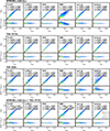 |
Fig. 4. Measured photo-z values as a function of true redshift. GAMA galaxies with 13 < i < 18 (N = 5961) in the wide dataset are shown in this figure. The colors show the magnitudes of the galaxies, binned by one-magnitude intervals. From the first row, results from the SPHEREx full-sky data, 7DS WTS data, 7DS RIS data, and combined SPHEREx full-sky + 7DS WTS data are plotted. Each plot has a subplot showing Δz/(1 + ztrue) as a function of ztrue. The statistics for measuring photo-z evaluation performance, NMAD (σ), bias (b), catastrophic failure (η, 10% outlier rate), and their corresponding errors, are noted in each plot. |
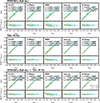 |
Fig. 5. Same as Figure 4, but for COSMOS galaxies with 18 < i < 21 (N = 990) in the wide dataset. We note that the redshift and magnitude ranges of the sample are different from those in Figure 4. |
Figure 4 shows the distribution of measured photo-z values from different methods and different survey combinations for the bright (13 < i < 18) GAMA galaxies as a function of true redshifts. To enable robust comparison between the template-fitting methods and ML-based methods, we used only the galaxies in the test sample for the figures. In Figure 4, the distribution of photo-z values shows strong one-to-one correlations with the true redshifts of the mock SEDs, although the scatter of the resulting photo-z values is different for different combinations of methods and data. The brighter galaxies show a tighter one-to-one correlation compared to the fainter ones in all the plotted combinations of surveys and methods. The values of statistics are σ ≲ 0.005, b ≲ 0.005, and η ≲ 0.005 across all the combinations of methods and surveys presented in Figure 4, with the best case reaching down to 0.23% accuracy.
Figure 5 shows the measured photo-z values as a function of true redshifts for the COSMOS galaxies with 18 < i < 21 in the wide dataset. We used only the galaxies in the test sample. As in Figure 4, we plotted the results for each combination of methods and surveys separately. The combined SPHEREx and 7DS data show σ ∼ 0.015, |b|∼0.003, and η ∼ 0.003 for all the methods used, with the best case showing 0.71% accuracy. We did not have measurements from the DNN method for COSMOS galaxies, as the DNN method was affected by many nondetections in the faint galaxies (see Section 3.5).
Table 2 demonstrates that the overall results from the deep dataset were better than those from the wide dataset. The i band magnitude limit of 23 is comparable to the median depth of the deep sample. Therefore, Table 2 shows roughly similar statistics to the galaxies with 18 < i < 21 in the wide dataset, which are summarized in Figure 5. In other words, the deep dataset showed comparable photo-z performance to the wide dataset, even after including the galaxies that were fainter by two magnitudes.
When we excluded outliers for estimating the photo-z statistics, the σ for the COSMOS SPHEREx + 7DS sample with 18 < i < 23 improved by about 30%, for example. This suggests that we can improve photo-z performance significantly if we can identify outliers in advance. The development of schemes for identifying outliers is being considered.
4.2. Magnitude dependence of photo-z performance
As we noted in the previous section, the resulting performance of photo-z is strongly dependent on the magnitudes of the galaxies. In this regard, we plotted the statistics as a function of i band magnitudes in Figures 6 and 7 using the wide dataset for GAMA (13 < i < 18) and COSMOS (18 < i < 23) galaxies, respectively. We used only test samples for these figures to enable comparison between the ML-based methods and template-fitting methods, as we did in Figures 4 and 5. We plotted σ, b, and η in different columns. We showed the results of different survey data in the different rows of the figure. The methods are differentiated by the colors.
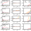 |
Fig. 6. Statistics of photo-z values as a function of i-magnitude. The GAMA galaxies within the wide dataset were used for calculating statistics. From the first row in the figure, we plotted the statistics from the SPHEREx full-sky, 7DS WTS, 7DS RIS, and combined SPHEREx full-sky + 7DS WTS data from the first row to the bottom. The statistics from different methods are plotted with different colors, which are noted in the legend. The shaded region interpolates the confidence intervals of the bins. |
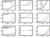 |
Fig. 7. Similar to Figure 6, but for the fainter COSMOS galaxies within the wide dataset. We plotted the results from the SPHEREx full-sky, 7DS WTS, and combined SPHEREx full-sky + 7DS WTS data from the first row. We note that the magnitude ranges and y limits are different from those in Figure 6. |
Figure 6 shows the dependence of the photo-z performance as a function of i magnitudes for the GAMA galaxies in the wide dataset. As they already provide sufficient signal to the SPHEREx full-sky and 7DS WTS surveys even for the faintest target plotted (i ≈ 18), they show more precise and robust photo-z estimates compared to the fainter COSMOS galaxies. Also, the trend between the statistics and i magnitudes is mostly flat, except for some cases like the σ of SPHEREx data when using the RF method or the η values from SPHEREx in-house code for 7DS-only data. The results from the RIS data also show comparable statistics to the deeper WTS data.
In Figure 7, we plotted the relation between the photo-z statistics and i magnitudes for the COSMOS galaxies in the wide dataset. We did not measure the photo-z for the COSMOS sample with the DNN method because of the difficulty of handling many nondetections (see Section 3.5). The relation between i-magnitude and the statistics in Figure 7 clearly shows the dependence of photo-z estimation performance on the S/N of the data. When only the SPHEREx data were used for photo-z estimation, the statistics become worse for the galaxies with i > 21, as it is below the detection threshold (See Figure 1). The 7DS data shows a comparable level of statistics to the SPHEREx data, although the statistics from different methods show larger scatter. For SPHEREx + 7DS data, the b, σ, and η are stable for the galaxies with i < 22, exhibiting better performance compared to either 7DS- or SPHEREx-only data.
4.3. Redshift dependence of photo-z performance
We plotted the dependence of the measured statistics on the true redshifts (ztrue) in Figure 8. In this figure, we used the results of COSMOS galaxies in the wide dataset with 18 < i < 21. We calculated statistics of the galaxies within each bin of the true redshift (Δztrue = 0.1). We calculated the statistics only for bins containing more than 70 galaxies to ensure robust estimation. We used the galaxies within the test sample for fair comparison between the ML-based and template-fitting methods.
The results in the last row from the combined SPHEREx + 7DS data showed the lowest σ, |b|, and η across all true redshifts plotted in the figure. All methods plotted in the figure exhibit the improved statistics for the combined dataset compared to either the SPHEREx or 7DS dataset. We further discuss the synergy between the SPHEREx and 7DS in Section 5.2.
5. Discussion
5.1. Photo-z with SPHEREx and 7DS
The SPHEREx and 7DS surveys densely sample galaxy SEDs from optical to near-infrared wavelengths without spectral gaps, covering hundreds of millions of galaxies across wide sky areas without target preselection. In this study, we forecasted the precision and accuracy of photo-z measurements from these surveys using simulated datasets.
The continuous sampling of SEDs significantly enhances the highest achievable precision of photo-z values, particularly for bright galaxies with enough S/N for relatively narrow bandwidths. Therefore, our results show σ, |b|, and η values lower than 0.01 for all the survey combinations and most of the methods when we measured photo-z values of GAMA galaxies (13 < i < 18, see Figure 4) within the wide dataset (SPHEREx full-sky + 7DS WTS).
Furthermore, the SPHEREx full-sky survey and RIS show comparable photo-z measuring performance to deeper WTS or combined SPHEREx full-sky + WTS, despite their relatively shallower depths (see Figure 6). As the surveys will cover up to full-sky area (SPHEREx full-sky, ∼40 000deg2) and our GAMA sample (N ∼ 30 000 for 13 < i < 18) spans ∼200deg2 in the sky, the surveys will cover up to ≲6 millions of similarly bright galaxies across the sky and provide photo-z values with subpercent precision and accuracy.
The statistics from the deep dataset show comparable results even when we include fainter galaxies with i ≲ 23, reflecting the enhanced S/N of deep surveys (Table 2). The values reveal that SPHEREx data show greater improvements compared to 7DS data when comparing the results between the wide and deep datasets. SPHEREx data exhibit about a 10–27 times smaller scatter, while 7DS data show about a 4–10 times improvement in scatter. When we compared the statistics from the deep SPHEREx and 7DS datasets, SPHEREx outperformed 7DS in photo-z performance. Although SPHEREx has shallower depth in its individual bandpasses, it benefits from approximately five times as many bandpasses as 7DS, as well as wavelength coverage that is about ten times broader. These factors collectively enhance the photo-z measurements of SPHEREx.
The dense SED sampling also facilitates robust characterization of continuum features, making the photo-z estimation more reliable for passive galaxies compared to star-forming galaxies. When we analyzed the statistics as a function of rest-frame B − V colors, the statistics were slightly better for redder galaxies consistently across most survey configurations.
Our result is generally consistent with Feder et al. (2024) using the SPHEREx, DECaLS (Dey et al. 2019) g r z, and WISE W1/W2 synthetic photometry. They reported σ = 0.0091, b = −0.0012, and η = 0.026 for galaxies with 18.5 < W1 < 19.0. Our results demonstrate σ = 0.0118 ± 0.0011, b = −0.0002 ± 0.0027, and η = 0.0082 ± 0.0059 for galaxies in the corresponding magnitude range (19 < i < 20) when using the SPHEREx in-house code, confirming consistency with previous results. We note that an apple-to-apple comparison is impossible, as they calculated photo-z performance statistics as a function of W1 magnitudes and incorporated broadband fluxes.
Ko et al. (2025) also conducted photo-z measurement tests using mock 7DS catalog based on EL-COSMOS SEDs (Saito et al. 2020). They estimated σ = 0.004, b = −0.033, and η = 0.016 for WTS within the galaxies with 19 ≤ m625 < 20. Our photo-z measurements return σ = 0.0053 ± 0.0005, b = 0.0010 ± 0.0008, and η = 0.0000 ± 0.0000 for WTS within the galaxies with 18.5 < i < 19.5, which roughly corresponds to 19 ≤ m625 < 20. Therefore, our results are also consistent with Ko et al. (2025), although the direct comparison is hard to achieve due to the difference in the sample and the survey parameters.
This level of photo-z measurement performance was hardly achieved in conventional broadband wide-field surveys. For example, Tanaka et al. (2018) tested the photo-z estimations using Hyper Supreme-Cam Subaru Strategic Program (HSC-SSP) data with multiple ML-based and template-fitting methods. Using five broadband photometric data (g, r, i, z, y), they achieved σ ∼ 0.02, b ∼ 0.002, and η ∼ 0.05 for galaxies with i ∼ 20 (see Table 2 of Tanaka et al. 2018). As they used deeper data than our wide dataset with a 5σ point source depth of r ∼ 26, the measured statistics remained similar down to i ∼ 23. However, the measured statistics from Tanaka et al. (2018) do not improve for brighter galaxies with i ≲ 19, for which our results still show some improvements compared to galaxies with i ∼ 20. The HSC-SSP provides deeper data compared to other surveys such as SDSS (York et al. 2000; Domínguez Sánchez et al. 2022) or Pan-STARRS1 (Chambers et al. 2016). Therefore, we can expect more improvements between our results and the photo-z values based on these data, although it is not straightforward to directly compare the results.
Ko et al. (2025) also conducted a comparison between the photo-z performance of the Pan-STARRS1 survey and mock 7DS data using EAZY (Brammer et al. 2008). They also found that the measured η and σ are significantly better when they used 7DS data. They found that photo-z values from Pan-STARRS1 can deviate from their true redshifts even when the target is much brighter (r < 20) than the limiting magnitudes of the survey (≲22.5, cf. Figure 1).
Furthermore, when Ko et al. (2025) combined the 7DS WTS and Pan-STARRS1 data for photo-z measurement, they found improvements by a factor of two in the statistics for the faint targets (m625 > 22), although the catastrophic failures remained unchanged. They interpreted it as the complement of the signal by relatively deeper PS1 surveys. This result also demonstrates the potential synergy between the medium-band surveys and deeper broadband surveys such as LSST (Ivezić et al. 2019), DESI (Dey et al. 2019), and Euclid (Laureijs et al. 2011).
5.2. Synergy between SPHEREx and 7DS
The photo-z statistics are persistently better in the combined dataset than in the SPHEREx-only or 7DS-only dataset, demonstrating the synergy between SPHEREx and 7DS in photo-z estimations. Figures 6 and 7 clearly show that the statistics of photo-z measurements are the best for the combined data (the last row of the figures) compared to others, for most of the photo-z methods. The difference is more distinct for the galaxies within the fainter magnitude bins. For example, when we compare the results from SPHEREx-only and SPHEREx + 7DS, Figure 7 shows that the combined dataset shows ∼5 times lower σ, ∼80 times lower |b|, and ∼8 times lower η for the galaxies with i ∼ 21.5. On the other hand, when we compare the results from 7DS-only and combined SPHEREx + 7DS data, the combined dataset shows comparable σ, but shows ∼7 times lower |b| and ∼4 times lower η for the same magnitude bin.
The results imply that SPHEREx data contribute to photo-z estimates, especially for b, even at the magnitude bins below the 5σ depths of the SPHEREx full-sky survey within the wide dataset. This is because the combination of SPHEREx and 7DS enhances the wavelength coverage. The combination thus can lift the degeneracy between color and redshift and reduce confusion from the low S/N data, making the photo-z measurements better. This is consistent with previous results (Feder et al. 2024; Ko et al. 2025), which showed that combining ancillary data with the survey spanning the wavelength range improved the photo-z performance.
Figures 5 and 7 show that the improvement of the results from the SPHEREx to the SPHEREx + 7DS results is more pronounced compared to the difference between the 7DS and SPHEREx + 7DS data. This difference is due to the higher S/N of WTS data, especially around galaxies with i ∼ 21, which are between the depth of WTS and the SPHEREx full-sky survey. For the brighter galaxies in which WTS and the SPHEREx full-sky survey have enough signal, the statistics from SPHEREx and 7DS data become more similar (see Figure 4).
Feder et al. (2024) noted that the forecasted photo-z performance of SPHEREx already meets its planned science requirements. Therefore, our results demonstrate the potential of the combined 7DS and SPHEREx data that can yield contributions to the planned sciences beyond the expected levels. For example, the improved photo-z estimations can help probe the large-scale structures and clustering of the galaxies. We can also use this distance information for multimessenger astronomy, such as inferring host galaxies of gravitational wave events by matching their localization area and redshift peaks in galaxy catalogs (Singer et al. 2016; Dálya et al. 2018) or by assigning probabilities of hosting the events to the galaxies using redshift and other parameters, for example, stellar mass (Del Pozzo 2012; Gair et al. 2023; Jeong & Im 2024).
The combination of SPHEREx and 7DS also reduces the dependence of photo-z performance on the true redshifts. Figure 8 shows general improvements of the statistics in the combined dataset when we calculated the statistics of the galaxies within the true redshifts. The statistics from SPHEREx data show lower performance compared to SPHEREx + 7DS data, especially for the galaxies with low redshifts. The 7DS statistics show better results at low redshift, but it also has a larger b compared to the combined data. The longer wavelength coverage of the combined dataset can detect more spectral features and prevent confusion of the spectral features. For example, low-redshift galaxies will lack some spectral features useful for identifying photo-z values such as the 4000 Å break or strong Hα line in the SPHEREx data. On the other hand, SPHEREx can capture the 1.6 μm bump and some PAH emissions, complementing the photo-z estimation.
5.3. Comparison between the methods
The performance of the photo-z measurement is also dependent on the photo-z methods. In Figures 4 and 5, we plotted the results from different methods in the different columns. From Figures 6 to 8, we distinguish the methods with different colors. We note that some differences are marginal, as only a few deviations of photo-z measurements can yield this level of variation in statistics. Therefore, we focus on our discussion on the differences between methods that persistently appear across multiple sets of input data. In the discussion, we aim to offer insights for refining photo-z measurement strategies using SPHEREx, 7DS, or a combined dataset.
The SPHEREx in-house code (Stickley et al. 2016; Feder et al. 2024, also see Section 3.1) shows better results compared to other methods for the SPHEREx-only and SPHEREx + 7DS datasets in many cases. This result is also evident in Figures 6 and 7, where the orange lines representing the in-house code consistently exhibit superior statistical performance in the first row (SPHEREx full-sky data), especially for the fainter galaxies with i ≳ 21. However, the code shows worse b and η for 7DS-only data and worse η for SPHEREx + 7DS data compared to other methods for faint galaxies with i ≳ 20.
When we compare the SPHEREx in-house code with LePhare, Figures 6 to 8 shows that they have distinct trends of statistics as a function of magnitudes and redshifts from LePhare. For example, Figure 5 shows that LePhare and the SPHEREx in-house code have notable differences for galaxies with 22 < i < 23 when using 7DS-only data. The SPHEREx in-house code shows larger b, σ, and η in this magnitude bin (see the 3rd row of Figure 7).
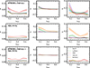 |
Fig. 8. Statistics of photo-z values as a function of true redshifts (ztrue). COSMOS galaxies with 18 < i < 21 in the wide dataset were used to calculate the statistics. The number of galaxies within each ztrue bin is higher than 70. From the first row in the figure, we plotted the statistics from SPHEREx, 7DS, and SPHEREx + 7DS data. The shaded regions interpolate the confidence intervals of the bins. |
The LePhare and SPHEREx in-house codes were different in the application of dust extinction laws, although the codes shared a similar template-fitting algorithm and the same template spectra. As we noted in Section 3.1, the in-house code incorporated the dust extinction laws into the model grid. We did not apply the additional dust extinction to LePhare (see Section 3.4). The dust extinction laws in the SPHEREx model introduce additional flexibility to the template spectra for the fitting. Although LePhare applies a coarser grid size than the in-house code, we confirmed that the different grid sizes (0.002 vs. 0.005) do not significantly affect the photo-z performance.
The lower performance of the SPHEREx in-house code for 7DS data compared to LePhare can be attributed to the relative difficulty of constraining the dust extinction in the 7DS wavelength range alone. The additional flexibility from the dust extinctions introduces degeneracy with the redshifts. On the other hand, broad NIR wavelength coverage contains more continuum features like 1.6 μm bump and in long wavelength the spectral features are less susceptible to the extinction, making the redshift and extinction less degenerate to each other. This result shows the importance of the treatment of dust extinctions on photo-z estimations and wide wavelength coverage to constrain the dust extinctions. The two methods show similar levels of performance for the brighter galaxies, implying that this effect is more important for fainter galaxies.
The results from EAZY and eazy-py are more similar to each other than LePhare and the SPHEREx in-house code. They had some differences in the redshift grid, the detailed prescription of magnitude priors, the amplitude of constant template error (5% for EAZY, 1% for eazy-py), and the applied sets of templates. However, they shared many aspects like treatment of dust extinction or application of magnitude prior and the template-fitting algorithm, resulting in very similar statistics. Considering that the operation time for the original EAZY code was much faster than eazy-py, when needing photo-z estimations for large data, the EAZY code will be more appropriate to apply. On the other hand, when we need more flexibility, eazy-py code will be more recommendable.
Since we constructed a magnitude-redshift prior for EAZY using COSMOS galaxies while employing the built-in priors for eazy-py, the statistics from EAZY may be overestimated for COSMOS galaxies. However, because other configurations also differed between EAZY and eazy-py, it is not straightforward to conclude that the prior alone causes the observed differences in results. Nevertheless, we emphasize that SPHEREx and 7DS surveys require more optimized and independent priors to achieve better photo-z estimations.
5.3.1. Probability density functions
The template-fitting codes provide probability density functions (PDFs). They are a valuable measure for checking the sanity and credibility of the fitting. The codes also measure the confidence interval of the photo-z values using the PDFs (Arnouts et al. 1999; Brammer et al. 2008; Stickley et al. 2016; Brammer 2021). In this section, we compare the PDFs of the four template-fitting codes by the metric named PIT (Probability Integral Transform, Polsterer et al. 2016). We calculated the PIT of the samples using the following equation from Tanaka et al. (2018):
 (8)
(8)
We calculated the PIT values for COSMOS galaxies with 18 < i < 21 applying no cuts on FLAG_ML. The results based on the photo-z estimates from the combined SPHEREx + 7DS data are shown in Figure 9. The overall uniform distribution of the PIT values indicates that the PDFs are generally well calibrated, implying that the PDFs from the codes are reasonably well sampled and reflect the underlying uncertainties of the photo-z estimates. The peaks near PIT values of zero and one correspond to outliers where the true redshifts deviate significantly from the redshifts where the corresponding PDFs are located. EAZY and the in-house code exhibit a mildly convex distribution, suggesting underdispersed PDFs (Polsterer et al. 2016), whereas LePhare and eazy-py produce flatter PDFs, although the differences between the codes are not substantial.
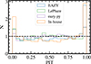 |
Fig. 9. Histogram of calculated PIT (Eq. (8)) from the PDFs of different template-fitting methods. We used COSMOS galaxies in the SPHEREx + 7DS wide dataset with 18 < i < 21. |
5.3.2. Comparison between confidence intervals
We assess the credibility of the estimated confidence intervals of template-fitting methods by comparing them with the real scatter between the photo-z values and the true redshift values. The reliability of the error estimates is important, as in real observations, we do not know the true redshifts. For this analysis, we used the results obtained from the SPHEREx + 7DS dataset for COSMOS galaxies in the wide-depth sample, including the training sample.
In Figure 10, we show the relation between the estimated redshift fractional uncertainties ( , where
  is half of the reported 68 % confidence interval) and real scatter in the photo-z measurements, σ (NMAD in this study), and the outlier fraction, η. The intrinsic scatter in the photo-z measurements, σ, exhibits an approximately linear relation with
  . However, the estimated errors generally underestimate the real scatter, σ. This underestimation is more significant for brighter galaxies.
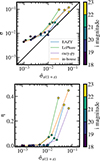 |
Fig. 10. σ as a function of the estimated redshift fractional uncertainties ( |

The underestimation of the confidence intervals in EAZY and the SPHEREx in-house code is consistent with the results from the PIT analysis. In contrast, LePhare shows a flat to mildly convex PIT distribution, implying overdispersed PDFs, yet yields underestimated confidence intervals. We attribute this to the multipeaked shape of the PDFs for some galaxies in LePhare. The presence of multiple peaks broadens the overall PDF, while the confidence intervals derived from the χ2 statistic in LePhare are typically confined to a single peak, leading to an underestimation of the confidence intervals.
As noted in Section 3.3, eazy-py in this study applies a correction factor of 1.5 to the flux uncertainties, which results in more consistent estimated errors to the real photo-z scatter compared to the other codes. The scaling behaves as expected for the fainter sample, as shown in the upper panel of Figure 10, because the sample for correcting flux errors is dominated by faint galaxies near the limiting magnitude of the data. The PIT distribution from eazy-py (purple histogram in Figure 9) also shows a flatter distribution compared to other codes. This suggests that the treatment of correcting uncertainties should account for the magnitude or S/N.
The lower panel of Figure 10 shows the outlier fraction (η) as a function of  . As expected, the outlier fraction increases with the estimated errors for all the codes. Generally, LePhare and the in-house code show a larger η compared to EAZY and eazy-py.
5.3.3. Notes on ML-based methods
In Figure 5, the results from HRF (Section 3.6, see also Kim et al. 2025b) show considerably lower scatter in the faintest magnitude bins for combined SPHEREx + 7DS and 7DS-only data. However, HRF shows larger scatter for bright galaxies, leading to relatively larger σ for GAMA galaxies (cf. Figure 4) for SPHEREx-only and SPHEREx + 7DS datasets.
To understand the distinct trend of the statistics as a function of magnitude, we investigated the photo-z measurements using the HRF method in more detail. As described in Section 3.6, HRF used flux uncertainties as input features in addition to the flux values. We built another HRF model without flux uncertainties for the wide dataset to check the dependence of photo-z measurement on the flux uncertainties. The resulting photo-z values show similar results to other methods for the SPHEREx + 7DS and 7DS data, with increased absolute values of the statistics for the faint magnitudes (21 < i < 23). The results from the SPHEREx data remain similar before and after removing flux uncertainties in the input features, but the HRF results are already similar to other methods for the dataset (see Figure 7).
These results imply that the flux uncertainty directly influences the redshift measurements in the HRF method, especially for objects with low S/N. The flux uncertainty does not affect the redshift estimation directly in the template-fitting methods, although a larger uncertainty leads to a smoother PDF and a larger photo-z uncertainty estimate. Using flux uncertainty to infer photo-z values may be helpful as we utilize additional information, provided that the survey is homogeneous enough to establish a reliable relationship between flux uncertainties and redshifts. However, when the survey is inhomogeneous, the information from the flux uncertainty can be biased, resulting in biased photo-z estimates depending on the training set. Therefore, to utilize flux uncertainties in the model, we should consider additional information that can affect the flux uncertainties, for example, the number of visits and the quality of the data.
The HRF method generally underperforms for bright galaxies compared to other methods, as shown in Figures 4 and 6. This likely originates from the HRF model’s limited capacity to extrapolate the inferred nonlinear relationships beyond the training set. To make HRF more accurate, we may need larger training samples spanning a wider range of redshifts and galaxy types.
The DNN method (Section 3.5) shows good performance for bright galaxies in these figures. Although it shows outstanding results for bright GAMA galaxies, the DNN method is difficult to apply to fainter targets with numerous nondetections (see Section 3.5). Since the data from the SPHEREx and 7DS surveys contain many bands that divide the signal more than broadband surveys, some nondetections are inevitable in the data. Therefore, to utilize DNN throughout the survey, we need to develop more robust methods for handling nondetections. Despite that, DNN will add reliable photo-z estimates to many bright galaxies.
6. Conclusion
In this paper we predicted the photo-z performance of the SPHEREx, 7DS, and combined SPHEREx + 7DS data by measuring photo-z values from SPHEREx and 7DS mock catalogs using six different photo-z methods. We summarize the main findings of this study as follows:
-
We constructed the mock catalogs of SPHEREx and 7DS surveys by convolving mock SEDs from Feder et al. (2024) with the SPHEREx and 7DS filter responses and considering observing conditions.
-
We tested photo-z measurement using EAZY, eazy-py, LePhare, SPHEREx in-house pipeline, HRF, and DNN. We provide results mainly for the SPHEREx full-sky + 7DS WTS (the wide dataset) and SPHEREx deep + 7DS IMS (the deep dataset).
-
For bright galaxies with 13 < i < 18 in the wide dataset (SPHEREx full-sky + 7DS WTS), the photo-z values show σ ≲ 0.005, b ≲ 0.001, and η ≲ 0.002 when we use the combined SPHEREx and 7DS data. We find σ ≲ 0.01, b ≲ 0.003, and η ≲ 0.01 for galaxies with 18 < i < 21 with the same survey combination. These results show significant improvements compared to the literature broadband-based photo-z results, especially for bright targets with enough S/N for the SPHEREx and 7DS bands.
-
The deep dataset (SPHEREx deep + 7DS IMS) shows comparable performance for galaxies that are up to two magnitudes fainter than those in the wide dataset.
-
The SPHEREx + 7DS combined dataset shows better results for almost all galaxies and methods, showcasing the synergy between the surveys. The photo-z values from the combined dataset also show a lower dependence on the magnitude and true redshift of the galaxies.
-
The methods show differences in photo-z performance, especially for faint galaxies. The SPHEREx in-house pipeline generally shows the best results for SPHEREx-only data and SPHEREx + 7DS data for galaxies with i ≲ 22.
-
Although they use the same template-fitting algorithm, LePhare and the SPHEREx in-house pipeline show different trends of statistics as a function of magnitudes and redshifts. The difference mainly comes from the application of dust extinction laws in the SPHEREx in-house code.
-
We show from the PIT analysis that the PDFs of the four template-fitting codes are generally well calibrated, but with a mild sign of underdispersed PDFs for the SPHEREx in-house code and EAZY. We also examined the estimated confidence intervals, which scale with the real scatter of the photo-z estimates, and found that boosting the flux uncertainties helps correct the tendency to underestimate the real scatter in the photo-z values.
-
The random forest method shows noticeably better results for faint galaxies in the combined SPHEREx + 7DS and 7DS-only data, specifically for faint galaxies with i > 22. However, this method exploits flux uncertainties for photo-z estimation, which can lead to bias for real data that may have some inhomogeneities.
-
The deep neural network method shows better statistics for bright galaxies, but its applicability is limited for fainter targets with many nondetections.
Our results demonstrate the capability of SPHEREx and 7DS to provide a large number of precise photometric redshifts. By comparing several widely used photo-z methods, we examined the main factors that influence photo-z performance and highlighted the complementary nature of the two surveys. The aim of this work is not to optimize individual codes or to identify a preferred method, but rather to assess how representative photo-z techniques respond to simulated SPHEREx and 7DS data in preparation for the upcoming observations. Owing to the unique characteristics of SPHEREx and 7DS, such as dense narrowband sampling, together with their anticipated synergy, the combined dataset shows improved performance compared to either survey alone. This study, therefore, provides a baseline expectation for photo-z measurements from future SPHEREx and 7DS observations.
Acknowledgments
We are grateful to the anonymous referee for giving valuable comments to improve the content of this paper. This work was supported by the National Research Foundation of Korea (NRF) grant, No. 2021M3F7A1084525, funded by the Korean government (MSIT). HSH acknowledges the support of Samsung Electronics Co., Ltd. (Project Number IO220811-01945-01), the NRF grant funded by the Korean government (MSIT), NRF-2021R1A2C1094577, and Hyunsong Educational & Cultural Foundation. Y. K. was supported by the NRF grant funded by the Korean government (MSIT) (No. 2021R1C1C2091550). B. L. is supported by the NRF grant funded by the Korea government(MSIT) (No. NRF-2022R1C1C1008695). M. K. was supported by the NRF grant funded by the Korean government (MSIT) (No. RS-2024-00347548). SL acknowledges support from the NRF grant (RS-2025-00573214) funded by the Korean government(MSIT). S. K. was supported by the NRF grant funded by the Korean government (MSIT) (No. 2022R1C1C2005539). The work of HB was supported by the Basic Science Research Program through the NRF funded by the Ministry of Education (RS-2025-25403440). D.K. acknowledges the support by the NRF grant (No. 2021R1C1C1013580) funded by the Korean government (MSIT). J.H.K. acknowledges the Institute of Information & Communications Technology Planning & Evaluation (IITP) grant, No. RS-2021-II212068 funded by the Korean government (MSIT).
References
- Allen, D. A. 1976, MNRAS, 174, 29P [NASA ADS] [Google Scholar]
- Almosallam, I. A., Jarvis, M. J., & Roberts, S. J. 2016, MNRAS, 462, 726 [Google Scholar]
- Arnouts, S., Cristiani, S., Moscardini, L., et al. 1999, MNRAS, 310, 540 [Google Scholar]
- Baum, W. A. 1962, IAU Symp., 15, 390 [Google Scholar]
- Beck, R., Dobos, L., Budavári, T., Szalay, A. S., & Csabai, I. 2016, MNRAS, 460, 1371 [Google Scholar]
- Benitez, N., Dupke, R., Moles, M., et al. 2014, arXiv e-prints [arXiv:1403.5237] [Google Scholar]
- Bernyk, M., Croton, D. J., Tonini, C., et al. 2016, ApJS, 223, 9 [NASA ADS] [CrossRef] [Google Scholar]
- Blake, C., & Bridle, S. 2005, MNRAS, 363, 1329 [Google Scholar]
- Bock, J. J., Aboobaker, A. M., Adamo, J., et al. 2025, arXiv e-prints [arXiv:2511.02985] [Google Scholar]
- Boris, N. V., Sodré, L., Jr, Cypriano, E. S., et al. 2007, ApJ, 666, 747 [NASA ADS] [CrossRef] [Google Scholar]
- Brammer, G. 2021, https://doi.org/10.5281/zenodo.5012704 [Google Scholar]
- Brammer, G. B., van Dokkum, P. G., & Coppi, P. 2008, ApJ, 686, 1503 [Google Scholar]
- Breiman, L. 2001, Mach. Learn., 45, 5 [Google Scholar]
- Brown, M. J. I., Moustakas, J., Smith, J. D. T., et al. 2014, ApJS, 212, 18 [Google Scholar]
- Bruzual, G., & Charlot, S. 2003, MNRAS, 344, 1000 [NASA ADS] [CrossRef] [Google Scholar]
- Calzetti, D., Armus, L., Bohlin, R. C., et al. 2000, ApJ, 533, 682 [NASA ADS] [CrossRef] [Google Scholar]
- Cappellari, M. 2017, MNRAS, 466, 798 [Google Scholar]
- Cardamone, C. N., van Dokkum, P. G., Urry, C. M., et al. 2010, ApJS, 189, 270 [Google Scholar]
- Carnero, A., Sánchez, E., Crocce, M., Cabré, A., & Gaztañaga, E. 2012, MNRAS, 419, 1689 [NASA ADS] [CrossRef] [Google Scholar]
- Carrasco Kind, M., & Brunner, R. J. 2013, MNRAS, 432, 1483 [Google Scholar]
- Castignani, G., & Benoist, C. 2016, A&A, 595, A111 [NASA ADS] [CrossRef] [EDP Sciences] [Google Scholar]
- Cha, S., Cho, B. Y., Joo, H., et al. 2025, ApJ, 987, L15 [Google Scholar]
- Chambers, K. C., Magnier, E. A., Metcalfe, N., et al. 2016, arXiv e-prints [arXiv:1612.05560] [Google Scholar]
- Cohen, J., & Cohen, P. 1975, in Applied Multiple Regression/correlation Analysis for the Behavioral Sciences (Lawrence Erlbaum) [Google Scholar]
- Collister, A. A., & Lahav, O. 2004, PASP, 116, 345 [NASA ADS] [CrossRef] [Google Scholar]
- Comparat, J., Delubac, T., Jouvel, S., et al. 2016, A&A, 592, A121 [NASA ADS] [CrossRef] [EDP Sciences] [Google Scholar]
- Coupon, J., Ilbert, O., Kilbinger, M., et al. 2009, A&A, 500, 981 [NASA ADS] [CrossRef] [EDP Sciences] [Google Scholar]
- Crill, B. P., Werner, M., Akeson, R., et al. 2020, SPIE Conf. Ser., 11443, 114430I [Google Scholar]
- Crill, B. P., Bach, Y. P., Bryan, S. A., et al. 2025, ApJS, 281, 10 [Google Scholar]
- Crocce, M., Carretero, J., Bauer, A. H., et al. 2016, MNRAS, 455, 4301 [NASA ADS] [CrossRef] [Google Scholar]
- da Cunha, E., Charlot, S., & Elbaz, D. 2008, MNRAS, 388, 1595 [Google Scholar]
- Dahlen, T., Mobasher, B., Faber, S. M., et al. 2013, ApJ, 775, 93 [Google Scholar]
- Dálya, G., Galgóczi, G., Dobos, L., et al. 2018, MNRAS, 479, 2374 [Google Scholar]
- Dawson, K. S., Kneib, J.-P., Percival, W. J., et al. 2016, AJ, 151, 44 [Google Scholar]
- De Lucia, G., & Blaizot, J. 2007, MNRAS, 375, 2 [Google Scholar]
- Del Pozzo, W. 2012, Phys. Rev. D, 86, 043011 [NASA ADS] [CrossRef] [Google Scholar]
- DESI Collaboration (Aghamousa, A., et al.) 2016, arXiv e-prints [arXiv:1611.00036] [Google Scholar]
- Dey, A., Schlegel, D. J., Lang, D., et al. 2019, AJ, 157, 168 [Google Scholar]
- Domínguez Sánchez, H., Margalef, B., Bernardi, M., & Huertas-Company, M. 2022, MNRAS, 509, 4024 [Google Scholar]
- Doré, O., Bock, J., Ashby, M., et al. 2014, arXiv e-prints [arXiv:1412.4872] [Google Scholar]
- Doré, O., Werner, M. W., Ashby, M., et al. 2016, arXiv e-prints [arXiv:1606.07039] [Google Scholar]
- Doré, O., Werner, M. W., Ashby, M. L. N., et al. 2018, arXiv e-prints [arXiv:1805.05489] [Google Scholar]
- Driver, S. P., Bellstedt, S., Robotham, A. S. G., et al. 2022, MNRAS, 513, 439 [NASA ADS] [CrossRef] [Google Scholar]
- Durret, F., Adami, C., Cappi, A., et al. 2011, A&A, 535, A65 [NASA ADS] [CrossRef] [EDP Sciences] [Google Scholar]
- Edge, A., Sutherland, W., Kuijken, K., et al. 2013, The Messenger, 154, 32 [NASA ADS] [Google Scholar]
- Eriksen, M., Alarcon, A., Gaztanaga, E., et al. 2019, MNRAS, 484, 4200 [NASA ADS] [CrossRef] [Google Scholar]
- Euclid Collaboration (Laigle, C., et al.) 2025, arXiv e-prints [arXiv:2503.15333] [Google Scholar]
- Euclid Collaboration (Scaramella, R., et al.) 2022, A&A, 662, A112 [NASA ADS] [CrossRef] [EDP Sciences] [Google Scholar]
- Feder, R. M., Masters, D. C., Lee, B., et al. 2024, ApJ, 972, 68 [Google Scholar]
- Gair, J. R., Ghosh, A., Gray, R., et al. 2023, AJ, 166, 22 [NASA ADS] [CrossRef] [Google Scholar]
- Gomes, Z., Jarvis, M. J., Almosallam, I. A., & Roberts, S. J. 2018, MNRAS, 475, 331 [NASA ADS] [CrossRef] [Google Scholar]
- Gunn, J. E., Siegmund, W. A., Mannery, E. J., et al. 2006, AJ, 131, 2332 [NASA ADS] [CrossRef] [Google Scholar]
- Hahn, C., Wilson, M. J., Ruiz-Macias, O., et al. 2023, AJ, 165, 253 [CrossRef] [Google Scholar]
- Henghes, B., Thiyagalingam, J., Pettitt, C., Hey, T., & Lahav, O. 2022, MNRAS, 512, 1696 [NASA ADS] [CrossRef] [Google Scholar]
- Hildebrandt, H., Viola, M., Heymans, C., et al. 2017, MNRAS, 465, 1454 [Google Scholar]
- Hook, I. M., Jørgensen, I., Allington-Smith, J. R., et al. 2004, PASP, 116, 425 [NASA ADS] [CrossRef] [Google Scholar]
- Ilbert, O., Arnouts, S., McCracken, H. J., et al. 2006, A&A, 457, 841 [NASA ADS] [CrossRef] [EDP Sciences] [Google Scholar]
- Ilbert, O., Capak, P., Salvato, M., et al. 2009, ApJ, 690, 1236 [NASA ADS] [CrossRef] [Google Scholar]
- Ilbert, O., McCracken, H. J., Le Fèvre, O., et al. 2013, A&A, 556, A55 [NASA ADS] [CrossRef] [EDP Sciences] [Google Scholar]
- Ivezić, Ž., Kahn, S. M., Tyson, J. A., et al. 2019, ApJ, 873, 111 [Google Scholar]
- James, G., Witten, D., Hastie, T., & Tibshirani, R. 2021, in An introduction to Statistical Learning, 2nd edn. (New York, NY: Springer) [Google Scholar]
- Jeong, M., & Im, M. 2024, ApJ, 974, 114 [Google Scholar]
- Khalouei, E., Shafieloo, A., Kim, A. G., et al. 2025, A&A, 698, A266 [NASA ADS] [CrossRef] [EDP Sciences] [Google Scholar]
- Kim, J. H., Im, M., Lee, H., et al. 2024, SPIE Conf. Ser., 13094, 130940X [Google Scholar]
- Kim, T., Sohn, J., & Hwang, H. S. 2025a, AJ, 170, 9 [Google Scholar]
- Kim, T., Sohn, J., Hwang, H. S., et al. 2025b, ApJS, 277, 41 [Google Scholar]
- Ko, E., Im, M., Lee, S.-K., & Laigle, C. 2024, ApJ, 976, 154 [Google Scholar]
- Ko, E., Im, M., Yang, Y., et al. 2025, ApJ, 994, 224 [Google Scholar]
- Koo, D. C. 1985, AJ, 90, 418 [NASA ADS] [CrossRef] [Google Scholar]
- Korngut, P. M., Bock, J. J., Akeson, R., et al. 2018, SPIE Conf. Ser., 10698, 106981U [Google Scholar]
- Kurtz, M. J., & Mink, D. J. 1998, PASP, 110, 934 [NASA ADS] [CrossRef] [Google Scholar]
- Laigle, C., McCracken, H. J., Ilbert, O., et al. 2016, ApJS, 224, 24 [Google Scholar]
- Laur, J., Tempel, E., Tamm, A., et al. 2022, A&A, 668, A8 [NASA ADS] [CrossRef] [EDP Sciences] [Google Scholar]
- Laureijs, R., Amiaux, J., Arduini, S., et al. 2011, arXiv e-prints [arXiv:1110.3193] [Google Scholar]
- Lawson, C. L., & Hanson, R. 1974, Solving least squares problems [Google Scholar]
- Lee, B., & Chary, R.-R. 2020, MNRAS, 497, 1935 [NASA ADS] [CrossRef] [Google Scholar]
- Lee, J. H., Park, C., Hwang, H. S., & Kwon, M. 2024, ApJ, 966, 113 [NASA ADS] [CrossRef] [Google Scholar]
- Lim, H., Shim, H., Im, M., et al. 2025, J. Korean Astron. Soc., 58, 43 [Google Scholar]
- Mandelbaum, R. 2018, ARA&A, 56, 393 [Google Scholar]
- Masters, D., Capak, P., Stern, D., et al. 2015, ApJ, 813, 53 [Google Scholar]
- McMahon, R. G., Banerji, M., Gonzalez, E., et al. 2013, The Messenger, 154, 35 [NASA ADS] [Google Scholar]
- Newman, J. A., & Gruen, D. 2022, ARA&A, 60, 363 [NASA ADS] [CrossRef] [Google Scholar]
- Noll, S., Kausch, W., Barden, M., et al. 2012, A&A, 543, A92 [NASA ADS] [CrossRef] [EDP Sciences] [Google Scholar]
- Oke, J. B., & Gunn, J. E. 1983, ApJ, 266, 713 [NASA ADS] [CrossRef] [Google Scholar]
- Paek, G. S. H., Im, M., Choi, H., et al. 2024, GRB Coordinates Network, 35790, 1 [Google Scholar]
- Pathi, I. M., Soo, J. Y. H., Wee, M. J., et al. 2025, JCAP, 2025, 097 [Google Scholar]
- Pedregosa, F., Varoquaux, G., Gramfort, A., et al. 2011, J. Mach. Learn. Res., 12, 2825 [Google Scholar]
- Polletta, M., Tajer, M., Maraschi, L., et al. 2007, ApJ, 663, 81 [NASA ADS] [CrossRef] [Google Scholar]
- Polsterer, K. L., D’Isanto, A., & Gieseke, F. 2016, arXiv e-prints [arXiv:1608.08016] [Google Scholar]
- Prakash, A., Licquia, T. C., Newman, J. A., & Rao, S. M. 2015, ApJ, 803, 105 [NASA ADS] [CrossRef] [Google Scholar]
- Prevot, M. L., Lequeux, J., Maurice, E., Prevot, L., & Rocca-Volmerange, B. 1984, A&A, 132, 389 [Google Scholar]
- Reid, B., Ho, S., Padmanabhan, N., et al. 2016, MNRAS, 455, 1553 [NASA ADS] [CrossRef] [Google Scholar]
- Ross, A. J., Bautista, J., Tojeiro, R., et al. 2020, MNRAS, 498, 2354 [NASA ADS] [CrossRef] [Google Scholar]
- Rudnick, G., Franx, M., Rix, H.-W., et al. 2001, AJ, 122, 2205 [Google Scholar]
- Saito, S., de la Torre, S., Ilbert, O., et al. 2020, MNRAS, 494, 199 [NASA ADS] [CrossRef] [Google Scholar]
- Salvato, M., Ilbert, O., & Hoyle, B. 2019, Nat. Astron., 3, 212 [NASA ADS] [CrossRef] [Google Scholar]
- Sánchez, E., Carnero, A., García-Bellido, J., et al. 2011, MNRAS, 411, 277 [CrossRef] [Google Scholar]
- Schlafly, E. F., Meisner, A. M., & Green, G. M. 2019, ApJS, 240, 30 [Google Scholar]
- Scoville, N., Aussel, H., Benson, A., et al. 2007, ApJS, 172, 150 [Google Scholar]
- Scoville, N., Arnouts, S., Aussel, H., et al. 2013, ApJS, 206, 3 [Google Scholar]
- Seo, H.-J., Ho, S., White, M., et al. 2012, ApJ, 761, 13 [NASA ADS] [CrossRef] [Google Scholar]
- Shuntov, M., Akins, H. B., Paquereau, L., et al. 2025, arXiv e-prints [arXiv:2506.03243] [Google Scholar]
- Singer, L. P., Chen, H.-Y., Holz, D. E., et al. 2016, ApJ, 829, L15 [NASA ADS] [CrossRef] [Google Scholar]
- Sohn, J., Geller, M. J., Hwang, H. S., et al. 2023, ApJ, 945, 94 [Google Scholar]
- Stickley, N. R., Capak, P., Masters, D., et al. 2016, arXiv e-prints [arXiv:1606.06374] [Google Scholar]
- Tanaka, M., Coupon, J., Hsieh, B.-C., et al. 2018, PASJ, 70, S9 [Google Scholar]
- Taylor, E. N., Franx, M., van Dokkum, P. G., et al. 2009, ApJS, 183, 295 [NASA ADS] [CrossRef] [Google Scholar]
- Treu, T. 2010, ARA&A, 48, 87 [NASA ADS] [CrossRef] [Google Scholar]
- Uomoto, A., Smee, S., Rockosi, C., et al. 1999, Am. Astron. Soc. Meeting Abstr., 195, 87.01 [Google Scholar]
- Virtanen, P., Gommers, R., Oliphant, T. E., et al. 2020, Nature Methods, 17, 261 [CrossRef] [Google Scholar]
- Wang, Y., Zhai, Z., Alavi, A., et al. 2022, ApJ, 928, 1 [Google Scholar]
- Weaver, J. R., Kauffmann, O. B., Ilbert, O., et al. 2022, ApJS, 258, 11 [NASA ADS] [CrossRef] [Google Scholar]
- Wittman, D., Bhaskar, R., & Tobin, R. 2016, MNRAS, 457, 4005 [Google Scholar]
- Wolf, C., Meisenheimer, K., Rix, H. W., et al. 2003, A&A, 401, 73 [NASA ADS] [CrossRef] [EDP Sciences] [Google Scholar]
- York, D. G., Adelman, J., Anderson, J. E., Jr, et al. 2000, AJ, 120, 1579 [Google Scholar]
- Zheng, H., & Zhang, Y. 2012, SPIE Conf. Ser., 8451, 845134 [Google Scholar]
- Zhou, R., Newman, J. A., Mao, Y.-Y., et al. 2021, MNRAS, 501, 3309 [NASA ADS] [CrossRef] [Google Scholar]
Depths from www.eso.org/rm/api/v1/public/releaseDescriptions/144
The mission’s data products will be publicly accessible through NASA’s Infrared Science Archive (IRSA).
All Tables
Statistics of the COSMOS galaxies in the wide (N = 34 531) and deep dataset (N = 219) with 18 < i < 23.
All Figures
|
Fig. 1. 5σ point source detection limits of SPHEREx surveys and 7DS. The colored squares show the depths of the three layers of 7DS, with the RIS at the top, followed by the WTS and IMS layers. The circular markers show the depths of SPHEREx full-sky and deep surveys from the top. The blue, red, green, and pale blue triangles denote the 5σ point source depths of other popular optical and NIR imaging surveys (SDSS York et al. 2000, unWISE Schlafly et al. 2019, VHS McMahon et al. 2013, and Pan-STARRS Chambers et al. 2016). The shaded regions show the wavelength ranges of the plotted broadband filters as labeled at the top: u, g, r, i, z, Y, J, H, Ks, W1, and W2. |
| In the text | |
|
Fig. 2. Redshift and i magnitude distribution of GAMA and COSMOS galaxies used in this work. The GAMA data (bright blue) consists of brighter galaxies (i ≲ 18.5) with low redshifts (z ≲ 0.4) compared to COSMOS galaxies (maroon) with 18 ≲ i ≲ 25 and z ≲ 6. |
| In the text | |
|
Fig. 3. Simulated SPHEREx and 7DS data used in this study. The gray plot shows the mock SED from Feder et al. (2024). The left column of the figure shows the simulated photometry of the deep dataset (SPHEREx deep + 7DS IMS) and the right column shows that of the wide dataset (SPHEREx full-sky + 7DS WTS), with the same example galaxies sorted in ascending i magnitudes. The blue markers show the mock datapoints from the 7DS, and the orange markers show the simulated SPHEREx datapoints. |
| In the text | |
|
Fig. 4. Measured photo-z values as a function of true redshift. GAMA galaxies with 13 < i < 18 (N = 5961) in the wide dataset are shown in this figure. The colors show the magnitudes of the galaxies, binned by one-magnitude intervals. From the first row, results from the SPHEREx full-sky data, 7DS WTS data, 7DS RIS data, and combined SPHEREx full-sky + 7DS WTS data are plotted. Each plot has a subplot showing Δz/(1 + ztrue) as a function of ztrue. The statistics for measuring photo-z evaluation performance, NMAD (σ), bias (b), catastrophic failure (η, 10% outlier rate), and their corresponding errors, are noted in each plot. |
| In the text | |
|
Fig. 5. Same as Figure 4, but for COSMOS galaxies with 18 < i < 21 (N = 990) in the wide dataset. We note that the redshift and magnitude ranges of the sample are different from those in Figure 4. |
| In the text | |
|
Fig. 6. Statistics of photo-z values as a function of i-magnitude. The GAMA galaxies within the wide dataset were used for calculating statistics. From the first row in the figure, we plotted the statistics from the SPHEREx full-sky, 7DS WTS, 7DS RIS, and combined SPHEREx full-sky + 7DS WTS data from the first row to the bottom. The statistics from different methods are plotted with different colors, which are noted in the legend. The shaded region interpolates the confidence intervals of the bins. |
| In the text | |
|
Fig. 7. Similar to Figure 6, but for the fainter COSMOS galaxies within the wide dataset. We plotted the results from the SPHEREx full-sky, 7DS WTS, and combined SPHEREx full-sky + 7DS WTS data from the first row. We note that the magnitude ranges and y limits are different from those in Figure 6. |
| In the text | |
|
Fig. 8. Statistics of photo-z values as a function of true redshifts (ztrue). COSMOS galaxies with 18 < i < 21 in the wide dataset were used to calculate the statistics. The number of galaxies within each ztrue bin is higher than 70. From the first row in the figure, we plotted the statistics from SPHEREx, 7DS, and SPHEREx + 7DS data. The shaded regions interpolate the confidence intervals of the bins. |
| In the text | |
|
Fig. 9. Histogram of calculated PIT (Eq. (8)) from the PDFs of different template-fitting methods. We used COSMOS galaxies in the SPHEREx + 7DS wide dataset with 18 < i < 21. |
| In the text | |
|
Fig. 10. σ as a function of the estimated redshift fractional uncertainties ( |
| In the text | |
Current usage metrics show cumulative count of Article Views (full-text article views including HTML views, PDF and ePub downloads, according to the available data) and Abstracts Views on Vision4Press platform.
Data correspond to usage on the plateform after 2015. The current usage metrics is available 48-96 hours after online publication and is updated daily on week days.
Initial download of the metrics may take a while.