| Issue |
A&A
Volume 706, February 2026
|
|
|---|---|---|
| Article Number | A180 | |
| Number of page(s) | 13 | |
| Section | Numerical methods and codes | |
| DOI | https://doi.org/10.1051/0004-6361/202557144 | |
| Published online | 11 February 2026 | |
New methods to improve the decontamination of slitless spectra
1
IRAP, Université de Toulouse, CNRS, CNES,
14 Av. Edouard Belin,
31400
Toulouse,
France
2
MatSim, Faculté des Sciences, Université Ibnou Zohr,
BP 8106 Cité Dakhla,
Agadir,
Maroc
★ Corresponding author: This email address is being protected from spambots. You need JavaScript enabled to view it.
Received:
8
September
2025
Accepted:
15
December
2025
Abstract
This paper proposes four new methods to decontaminate spectra of stars and galaxies resulting from slitless spectroscopy used in many space missions such as Euclid. These methods are based on two distinct approaches that simultaneously take into account multiple dispersion directions of light. The first approach, called the local instantaneous approach, is based on an approximate linear instantaneous model. The second approach, called the local convolutive approach, is based on a more realistic convolutive model that allows for the simultaneous decontamination and deconvolution of spectra. For each approach, a mixing model was developed to link the observed data to the source spectra. This was done either in the spatial domain for the local instantaneous approach or in the Fourier domain for the local convolutive approach. Four methods were then developed to decontaminate these spectra from the mixtures, exploiting the direct images provided by photometers. Test results obtained using realistic, noisy, Euclid-like data confirmed the effectiveness of the proposed methods.
Key words: methods: numerical / techniques: image processing / techniques: imaging spectroscopy
© The Authors 2026
 Open Access article, published by EDP Sciences, under the terms of the Creative Commons Attribution License (https://creativecommons.org/licenses/by/4.0), which permits unrestricted use, distribution, and reproduction in any medium, provided the original work is properly cited.
This article is published in open access under the Subscribe to Open model. This email address is being protected from spambots. You need JavaScript enabled to view it. to support open access publication.
1 Introduction
The aim of source separation is to recover a set of unknown signals, called sources, from a set of mixtures of these sources, called observations. When this estimation is done with minimal a priori information about the sources and the mixing parameters, it is referred to as blind source separation (BSS) (Comon & Jutten 2010; Hyvärinen & Oja 2000; Deville 2016). This approach has been receiving more attention recently thanks to the diversity of its fields of application, which includes audio processing (Makino 2018; Bella et al. 2022b), Earth observation (Bioucas-Dias et al. 2012; Heylen et al. 2014), biomedical applications (Zarzoso & Nandi 2001; Zokay & Saylani 2022), and astronomy (Meganem et al. 2015; Igual & Llinares 2007). In this paper, we address a new application of source separation concerning the decontamination of spectra resulting from slitless spectroscopy, a technique commonly used in various space missions such as James Webb Space Telescope (JWST) (Gardner et al. 2023), Hubble Space Telescope (HST), or in the Euclid space mission (Euclid Collaboration: Mellier et al. 2025). Our methods are specifically designed for Euclid-like configurations, but can also be adapted to other telescopes that use slitless spectroscopy, such as JWST and HST.
Euclid is a space telescope launched by the European Space Agency on July 1, 2023 (Euclid Collaboration: Mellier et al. 2025). Its primary objective is to understand the nature of dark energy and how it is responsible for the accelerating expansion of the Universe. Euclid will create a three-dimensional (3D) map of the Universe, with time as the third dimension. This map will represent millions of galaxies, revealing the evolution of the universe over time and providing crucial information about the nature of its accelerating expansion (Laureijs et al. 2011; Euclid Collaboration: Mellier et al. 2025). To achieve this goal, Euclid has been equipped with a slitless near-infrared spectro-photometer called NISP (Near Infrared Spectrometer Photometer) (Costille et al. 2019; Schirmer et al. 2022; Euclid Collaboration: Jahnke et al. 2025). NISP will measure the spectra of millions of galaxies. These spectra will then be analyzed to estimate the spectroscopic redshifts of the observed galaxies, focusing on the Hα line, which is usually the strongest emissionline in star-forming galaxies and thus the easiest to detect in the spectrum of a galaxy. The NISP instrument provides both direct nondispersed images from a photometer and dispersed images (corresponding to spectra) from a slitless spectrograph for all objects within the field of view. Photometry in NISP is performed using three filters, resulting in three near-infrared (NIR) photometric images in the three bands Y, J, and H (Euclid Collaboration: Jahnke et al. 2025).
The spectroscopy analysis is performed using grisms, which are a combination of prisms and diffraction gratings (Palmer & Loewen 2005). Each grism disperses the different wavelengths of the received light. In practice, several grisms can be used so that each grism disperses the received light in a specific dispersion direction (Euclid Collaboration: Jahnke et al. 2025). The output of the grism is a multi-row image, hereafter referred to as a spectrogram. Spectroscopy is usually performed with a slit that acts as a filter, allowing light to pass only from a small region of the sky containing a very limited number of objects. As a result, spectra from different sources can only be superposed if two or more objects are within the window defined by the slit. In contrast, slitless spectroscopy does not use a slit, which means that there is no filtering of sources, which allows a large number of objects to be observed in a single acquisition. Fig. 1 illustrates an example of two direct images of nearby astronomical objects, accompanied by their respective spectrograms after being dispersed by the grism. This figure clearly shows that slitless spectroscopy used leads to the superposition of spectrograms of astronomical objects (galaxies and stars). This superposition phenomenon is called contamination. It is important to note that the spectrogram of an object of interest can often be affected by several neighboring objects, which can lead to incorrect redshift estimates (Laureijs et al. 2011). Therefore, it is essential to use an effective decontamination method to minimize errors in redshift measurements (Hosseini et al. 2020).
To improve the efficiency of decontamination methods, multiple spectrograms are usually generated in different dispersion directions for the same field of view. In fact, when moving from one dispersion direction to another, the spectrum of an object of interest is often contaminated by different spectra. As a result, the simultaneous use of multiple dispersion directions provides a better estimate of the spectrum of the object of interest (Euclid Collaboration: Scaramella et al. 2022). For example, the Euclid observation strategy consists of generating spectrograms in four different dispersion directions, namely, 0, 180, 184, and −4 degrees. To achieve this, as illustrated in Fig. 2, two grisms with opposite dispersion directions (0 and 180 degrees) are used, each of which can be rotated by 4 degrees (Euclid Collaboration: Scaramella et al. 2022).
Spectra decontamination in slitless spectroscopy can be seen as a source separation problem. In this application, source separation can be achieved by either a local or a global approach. The main difference between these two approaches is that the local approach decontaminates objects one by one, while the global approach decontaminates all objects in a predefined zone simultaneously. Moreover, BSS methods have been employed in the literature to address various types of mixing models. In this paper, we focus on two distinct types: the linear instantaneous model and the convolutive model. For the linear instantaneous model, the observed signal at each wavelength is represented as a linear combination of the sources at the same detector position. In contrast, in the convolutive model, the observed signal at each wavelength is the result of the convolution of the sources with wavelength-dependent filters.
Since the treated spectra are neither mutually independent nor sparse, classical BSS methods based on independent component analysis (Comon & Jutten 2010; Hyvärinen & Oja 2000; Comon 1994) and sparse component analysis (O’grady et al. 2005; Bella et al. 2023; Gribonval & Lesage 2006) cannot be used. For this reason, most existing BSS methods for decontaminating slitless spectroscopy spectra exploit the positivity of the data (Selloum et al. 2015, 2016; Hosseini et al. 2020). However, these methods have several limitations:
They are mainly based on a non-negative matrix factorization (NMF) (Lee & Seung 1999), which is known to be very sensitive to initialization and do not guarantee the uniqueness of the solution;
They generally suffer from slow convergence;
In practice, they offer modest performance;
They do not use all the information available; particularly with respect to the existence of direct images provided by the photometers.
On the other hand, a basic slitless decontamination method for the HST was proposed in Kümmel et al. (2009). This method uses only one dispersion direction at a time and is based on estimating the continuum of the contaminants in the spectrogram of the object of interest by exploiting direct images of the contaminants. The estimated contaminant contributions are then summed to create a 2D contaminant image, which is subsequently subtracted from the spectrogram of the object of interest to obtain its uncontaminated spectrum. However, this method is only able to decontaminate the continuum component of the spectrogram and it cannot remove emission lines from contaminating objects nor unmodeled contaminants, such as hot pixels (Kümmel et al. 2009). Unlike this basic decontamination method, the GRIZLI pipeline (Brammer 2019) employs a more robust approach. While it similarly creates and subtracts contaminant models from direct images, GRIZLI refines the process by iteratively optimizing the contaminant’s spectral shape. This allows for the precise subtraction of both continuum and emission-line contributions from neighboring objects (Momcheva et al. 2016). Nevertheless, the GRIZLI approach has a fundamental limitation, as it cannot model contaminants that are undetected in the reference direct images. These contaminants remain a source of residual contamination. A distinct, matrix-based approach, known as LINEAR, was proposed by Ryan et al. (2018). Unlike the model-subtraction methods described above, LINEAR operates on a fundamentally different principle. Rather than constructing and subtracting individual source models, it frames the entire observed spectrogram as a large, sparse system of linear equations. In this system, each pixel is represented as a linear combination of contributions from every source in the field. Solving this system via regularized least squares enables the simultaneous extraction of all individual spectra. However, this method is highly computationally intensive, and its solution can be very sensitive to noise and the presence of unmodeled sources.
Due to the above-mentioned limitations of existing separation methods in slitless spectroscopy, this paper proposes four new separation methods adapted to Euclid-like spectra. These methods can also be used in other slitless spectroscopy applications and are based on two different local approaches. The first approach, called the local instantaneous approach, is based on a linear instantaneous model. The second, called the local convolutive approach, is based on a more realistic convolutive model that allows simultaneous decontamination and deconvolution of spectra. The proposed methods provide several practical advantages compared with model-subtraction techniques (basic, GRIZLI) and global inversion frameworks such as LINEAR. In particular, we focus on the following features.
Parallelism: The local nature of our models allows them to be run in parallel across many processors. This means we can decontaminate a large number of objects at the same time, unlike global approaches such as LINEAR, which require solving a single large system for the entire field.
Robustness to unmodeled sources: Our methods can mitigate contamination from faint or undetected sources in the reference images, addressing a fundamental and persistent limitation of other techniques.
Multidirectional exploitation: Our models explicitly and simultaneously use the four available dispersion directions. This integrated approach improves decontamination accuracy compared to methods that process each direction independently.
The proposed methods are partly described in our two conference papers (Bella et al. 2022a, 2024). The present paper provides a more complete description of these two approaches, as well as additional experimental results.
The remainder of this article is organized as follows: Sect. 2 presents the data models used in our work, as well as the two resulting mixing models. Sect. 3 presents in detail the proposed decontamination methods. Sect. 4 evaluates the performance of these methods. Finally, Sect. 5 provides a conclusion and perspectives for our work.
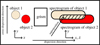 |
Fig. 1 Contamination of the spectra of neighboring objects at the output of the grism. |
 |
Fig. 2 Euclid ’s observation strategy. |
2 Data models
In this section, we present the physical model used in our work, along with two resulting mixing models that link the observed data to the source spectra. The first model is an approximate linear instantaneous model, which we used in our instantaneous methods presented in Sect. 3.1. The second model is a convolu-tive model, which we used in our convolutive method described in Sect. 3.2.
2.1 Observation model
Assuming that the spectral distribution of any astronomical object (galaxy or star) with index j is uniform at every point on the object, the light intensity of that object at a given point with coordinates (x, y) and wavelength λ can be modeled as
 (1)
(1)
where Sj(λ) is the spectrum of the object and fj(x, y) is its spatial intensity profile.
The modeling of the light intensity in Eq. (1) must take into account the convolution of the observed object with the point spread function (PSF) of the instrument. If we assume that the PSF is independent of the wavelength1, the new intensity of the observed object can be defined by the following equation,
![Mathematical equation: \begin{aligned}[b] w_j( x , y , \lambda)&=q_j(x,y,\lambda)* h( x , y )\\ &=s_j (\lambda ) [f_j ( x, y )* h( x , y )], \end{aligned}](/articles/aa/full_html/2026/02/aa57144-25/aa57144-25-eq2.png) (2)
(2)
where h represents the PSF of the instrument, and “*” is the convolution operator.
If we assume that the light emitted by the object described in Eq. (2) is then dispersed by a grism in the horizontal direction x, we would obtain a 2D dispersed image at the grism output for an object with an index, j. This corresponds to the spectrogram of this object (Hosseini et al. 2020; Freudling et al. 2008):
 (3)
(3)
where Ωλ is the wavelength range covered by the grism, and D(λ) is the grism dispersion function, which is the shift on the detector relative to a reference position as a function of wavelength in the dispersion direction x (Hosseini et al. 2020).
Assuming that the grism dispersion function is expressed in the linear form D(λ) = αλ + β (where α and β are two known coefficients), Eq. (3) becomes
![Mathematical equation: \begin{aligned}[b] t_j( x , y )&=\int_{\Omega_\lambda}^{}w_j( x-\alpha \lambda-\beta , y , \lambda)\;\mathrm{d}\lambda\\ &=\int_{\Omega_\lambda}^{}I_j( x-\alpha \lambda-\beta , y)\;s_j(\lambda)\;\mathrm{d}\lambda, \end{aligned}](/articles/aa/full_html/2026/02/aa57144-25/aa57144-25-eq4.png) (4)
(4)
where Ij(x, y) = fj(x, y) * h(x, y) is the object profile with index j convolved with the PSF of the instrument.
We note that the model (4) is a modified form of a convolution and represents the most accurate model among those used in our work. In Sect. 2.2, we present a simplified version of this model.
2.2 Local instantaneous mixing model
In the local instantaneous approach, the model in Eq. (4) is simplified by assuming the following separability assumption,
 (5)
(5)
This assumption means that the function Ij(x,y) is separable into x and y. According to Selloum et al. (2016); Hosseini et al. (2020), this assumption is more realistic for small or point-like objects, as well as for circular and elliptical objects oriented in the x or y directions. However, for other objects, an approximation error that depends on the shape of the object is introduced in our model (Selloum et al. 2016; Hosseini et al. 2020). Taking into account the assumption (5), Eq. (4) becomes in the dispersion direction di2
 (6)
(6)
The observed value for a pixel with index p = [n, m] in the dispersion direction di is expressed as follows
 (7)
(7)
where Ωp is the area of pixel p. If we replace  by its definition (6), we get
 (8)
(8)
with
 (9)
(9)
and
 (10)
(10)
Note that the value of  is independent of the vertical coordinate of the pixels m, and that the value of
  is independent of the horizontal coordinate of the pixels n.
Now consider a rectangular area containing the observed spectrogram of an object of interest, in the dispersion direction di. Each pixel of this spectrogram receives light from Ni objects (the object of interest and N - 1 contaminants). In this case, the observed value in each pixel of this spectrogram can be expressed as follows
 (11)
(11)
The mixing model (11) can then be expressed in the following linear instantaneous form
 (12)
(12)
where X(di) is the observation matrix of size Mi × K whose element (m, n) is o(di)(n, m), Mi represents the number of rows in the cross-dispersion direction associated with the spectrogram of the object of interest and K is the number of spectral bands, which is considered identical for all dispersion directions. ![Mathematical equation: ${\bf A}^{(i)}=\left[ {\bf a}_s^{(i)}|{\bf A}_c^{(i)}\right] $](/articles/aa/full_html/2026/02/aa57144-25/aa57144-25-eq16.png) is the mixing matrix of size Mi × Ni, defined by
is the mixing matrix of size Mi × Ni, defined by
 (13)
(13)
where ![Mathematical equation: ${\bf a}_s^{(i)}=[a_{1}^{(d_i)}(1), ..., a_{1}^{(d_i)}(M_i)]^T$](/articles/aa/full_html/2026/02/aa57144-25/aa57144-25-eq18.png) is the mixing vector of the object of interest, T denotes the transpose, Ni - 1 is the number of contaminants considered in the direction di, and
is the mixing vector of the object of interest, T denotes the transpose, Ni - 1 is the number of contaminants considered in the direction di, and  is the contaminant mixing matrix. As for E(i), it is the matrix of sources of size Ni × K, where the first row contains the vector e1, corresponding to a convolved version of the spectrum of the object of interest, while the other rows contain convolved versions of the spectra of contaminants in the direction di.
As mentioned in Sect. 1, we have four observations for each object of interest, corresponding to the four dispersion directions (0, 180, 184, and −4 degrees). Assuming that the spectrum of the object of interest remains the same in all dispersion directions, we can combine these four observations to improve the estimation of its spectrum. However, before combining the spectrograms from these four directions, some preprocessing steps are necessary. First, it is necessary to rotate X(180), X(184), and X(−4) by 180, 184, and −4 degrees, respectively, so that they are aligned with the horizontal direction (Bella et al. 2022a, 2024). This preprocessing is essential to ensure that all wavelengths from all dispersion directions of the object of interest are horizontally aligned to facilitate their simultaneous exploitation.
Secondly, it is essential to resample (without changing the sampling rate) the four spectrograms in the dispersion direction to further align them in terms of wavelength. In fact, the extraction of a contaminated spectrogram from the full dispersed image of a detector is not perfect, since the same wavelength may be at the beginning, middle or end of a pixel, depending on the dispersion direction.
Finally, it is essential to inter-calibrate the flux of the four spectrograms in the four dispersion directions by multiplying them with relative correction factors. The goal of this preprocessing is to bring all spectrograms to a common instrumental flux scale (Markovic et al. 2017).
After applying these three preprocessings, we then define the total observation matrix X of an object of interest by concatenating its contaminated spectrograms in the four directions as
 (14)
(14)
where A = [as|Ac] is the total mixing matrix of a size M × N, with  , as is the mixing vector of the object of interest, defined by
![Mathematical equation: {\bf a}_s=[{\bf a}_s^{{(1)}^T},{\bf a}_s^{{(2)}^T}, {\bf a}_s^{{(3)}^T}, {\bf a}_s^{{(4)}^T}]^T,](/articles/aa/full_html/2026/02/aa57144-25/aa57144-25-eq22.png) (15)
(15)
and Ac is the contaminant mixing matrix. Assuming the contaminants are different in each dispersion direction, this matrix can be written as
 (16)
(16)
E is the matrix of size N × K containing convolved version of the spectrum of the object of interest in its first row and convolved versions of the spectra of contaminants in each of the four directions in the following rows. It should be noted that if all contaminants are considered, the mixing matrix A might become underdetermined (i.e. M < N). In this case, we retain only the brightest contaminants in the four dispersion directions, so that the mixing matrix A becomes (over)-determined (i.e. M ≥ N). In Sect. 3.1, we present three methods that can be used to estimate the spectrum of the object of interest by exploiting the observation matrix X and available information on the objects.
2.3 Local convolutive mixing model
We recall the expression of the spectrogram model, as presented in Eq. (3), for an object with index j dispersed in the horizontal direction x,
 (17)
(17)
where wj(x,y,λ) = [fj(x,y) * h(x,y)]Sj(λ). Note that this equation is valid for all dispersion directions di ∈ 0°, 180°, 184°, −4° after rotating the spectrograms for each direction according to their respective angles.
Eq. (17) can be simplified by calculating its Fourier transform (FT) in the spatial domain as
![Mathematical equation: \begin{aligned}[b] T_j( f_x , f_y )&=\text {FT}\left\{t_j( x , y )\right\}=\text{FT} \left\{\int_{\Omega_\lambda}^{}w_j( x-D(\lambda) , y , \lambda)\;\mathrm{d}\lambda \right\}\\ &=\int_{\Omega_\lambda}^{}W_j( f_x, f_y , \lambda) \mathrm{e}^{-\mathrm{i}2\pi f_x D(\lambda)} \; \mathrm{d}\lambda\\ &=F_j( f_x, f_y)\, H( f_x, f_y) \int_{\Omega_\lambda}^{} s_j(\lambda)\mathrm{e}^{-\mathrm{i}2\pi f_x D(\lambda)}\;\mathrm{d}\lambda, \end{aligned}](/articles/aa/full_html/2026/02/aa57144-25/aa57144-25-eq25.png) (18)
(18)
where Fj(fx, fy) and H(fx, fy) are the 2D Fourier transforms of fj(x, y) and h(x, y), respectively, and the variables fx and fy correspond to the spatial frequency components in the Fourier domain.
Considering a linear dispersion D(λ) = αλ + β (where α and β are two known coefficients), Eq. (18) becomes
![Mathematical equation: \begin{aligned}[b] T_j( f_x , f_y )&=G_j( f_x, f_y) \int_{\Omega_\lambda}^{} s_j(\lambda)\mathrm{e}^{-\mathrm{i}2\pi f_x \alpha\lambda}\;\mathrm{d}\lambda \, \mathrm{e}^{-\mathrm{i}2\pi f_x \beta}\\ &=G_j( f_x, f_y) \, S_j(\alpha f_x) \, \mathrm{e}^{-\mathrm{i}2\pi f_x \beta}, \end{aligned}](/articles/aa/full_html/2026/02/aa57144-25/aa57144-25-eq26.png) (19)
(19)
where Gj(fx, fy) = Fj(fx, fy) H(fx, fy) and Sj is the 1D Fourier transform of Sj. We note that Sj(αfx) does not depend on the vertical frequency coordinate, fy.
The observed value at a frequency indexed by (fx, fy) in the dispersion direction di is expressed as follows
 (20)
(20)
where Ni is the number of objects in the dispersion direction di. Using vector notations, Eq. (20) can be reformulated as a complex-valued linear instantaneous model at each horizontal frequency, fx,
 (21)
(21)
where ![Mathematical equation: ${\bf X}^{{(d_i)}}(f_x)=[O^{{(d_i)}}(f_x,f_y(1)),\cdots,O^{{(d_i)}}(f_x,f_y(M_i))]^{\rm T}$](/articles/aa/full_html/2026/02/aa57144-25/aa57144-25-eq29.png) is a vector of size Mi × 1 containing the observed data at the horizontal frequency fx, with Mi being the number of vertical frequencies in the cross-dispersion direction y. Mi can vary from one dispersion direction to another, and its value depends on the vertical extent of the object of interest in that dispersion direction. Since the sources can be freely rearranged, we assume throughout the rest of this article that the first source S1 (fx) is the source of interest, and that
is a vector of size Mi × 1 containing the observed data at the horizontal frequency fx, with Mi being the number of vertical frequencies in the cross-dispersion direction y. Mi can vary from one dispersion direction to another, and its value depends on the vertical extent of the object of interest in that dispersion direction. Since the sources can be freely rearranged, we assume throughout the rest of this article that the first source S1 (fx) is the source of interest, and that ![Mathematical equation: ${\bf S}^{(i)}( f_x)=[S_1(\alpha f_x),S^{(d_i)}_{2}(\alpha f_x),\cdots,S^{(d_i)}_{N_i}(\alpha f_x)]^{\rm T}$](/articles/aa/full_html/2026/02/aa57144-25/aa57144-25-eq30.png) is a vector of size Ni × 1 containing compressed versions of the Fourier transforms of the source spectra.
is a vector of size Ni × 1 containing compressed versions of the Fourier transforms of the source spectra.
![Mathematical equation: ${\bf A}^{(i)}(f_x)=\left[ {\bf a}_s^{(i)}(f_x)|{\bf A}_c^{(i)}(f_x)\right]\, \mathrm{e}^{-\mathrm{i}2\pi f_x \beta}$](/articles/aa/full_html/2026/02/aa57144-25/aa57144-25-eq31.png) is the mixing matrix of a size Mi × Ni, where [...|...] is the concatenation of two matrices,
is the mixing matrix of a size Mi × Ni, where [...|...] is the concatenation of two matrices, ![Mathematical equation: ${\bf a}_s^{(i)}(f_x)=[G_1^{(d_i)}(f_x,f_y(1)),\cdots,G_1^{(d_i)}(f_x,f_y(M_i))]^{\rm T}$](/articles/aa/full_html/2026/02/aa57144-25/aa57144-25-eq32.png) is the mixing vector of the object of interest at each horizontal frequency fx, and
is the mixing vector of the object of interest at each horizontal frequency fx, and  is the contaminant mixing matrix of size Mi × (Ni - 1), defined by
 (22)
(22)
We have four observations for each object of interest, corresponding to the four dispersion directions di ∈ {0°, 180°, 184°, −4°}. Since the spectrum of the object of interest is the same regardless of the dispersion direction, it is possible to combine these four observations to improve the estimation of its spectrum. We define the total observation vector X(fx) corresponding to the object to be decontaminated at each horizontal frequency fx by merging the Fourier transforms of its contaminated spectrograms in the four directions as follows
 (23)
(23)
where A(fx) is the total mixing matrix of size M × N, with  , defined by
 (24)
(24)
Finally, S(fx) is a vector of size N × 1 containing the Fourier transform of the spectrum of the object of interest at the horizontal frequency, fx, in its first row, followed by the Fourier transforms of the contaminant spectra at the horizontal frequency, fx, in each of the four directions in the following rows. This vector is defined as
![Mathematical equation: \begin{split} {\bf S}( f_x)=\ &[S_1(\alpha f_x),S^{(0)}_{2}(\alpha f_x),\cdots,S^{(0)}_{N_1}(\alpha f_x),S^{(180)}_{2}(\alpha f_x),\cdots,S^{(180)}_{N_2}(\alpha f_x),\\ &S^{(184)}_{2}(\alpha f_x),\cdots,S^{(184)}_{N_3}(\alpha f_x),S^{(-4)}_{2}(\alpha f_x),\cdots,S^{(-4)}_{N_4}(\alpha f_x)]^{\rm T}. \end{split}$}](/articles/aa/full_html/2026/02/aa57144-25/aa57144-25-eq38.png) (25)
(25)
It should be noted that prior to the combination of the spectrograms from the four directions, the three preprocessings (rotations, resampling and calibration) introduced in Sect. 2.2 must be applied to the spectrograms of the object of interest in the spatial domain.
3 Methods
3.1 Local instantaneous methods
The local instantaneous approach is based on the linear instantaneous mixing model introduced in Sect. 2.2 and exploits the direct images of the objects to estimate the spectrum of an object of interest. This approach provides the vectors ej defined in Eq. (10), which represent estimates of the spectra sj after convolution by a function depending on the object’s profile in the direction of dispersion. The aim here is to separate the spectra, not to deconvolve them.
3.1.1 Mixing matrix estimation
The first step, common to all the proposed local instantaneous methods, consists of estimating the mixing matrix A, using the direct image of the object of interest as well as those of its contaminants. As previously mentioned in Sect. 1, Euclid is also equipped with a photometer that provides three direct images in the three spectral bands Y, J, and H of all astronomical objects in the field of view (Laureijs et al. 2011). However, in this work, only direct images of the J band were available and so, they were used to estimate the mixing matrix. The direct image, denoted  , is defined for an object of index j in the dispersion direction, di, as the integral of the light intensity of the observed object in Eq. (2) over the spectral domain,
 (26)
(26)
where ΩJ represents the wavelength range covered by the J band and Ij(x, y) = fj(x, y) * h(x, y) is the profile of the object with index j convolved to the instrument’s PSF.
As illustrated in Fig. 3, the flux of the direct image is dispersed by a grism to produce its spectrogram, also known as a 2D spectrum. Assuming that the light conserves its flux after dispersion, the sum of the fluxes on the pixels of each row of the direct image is equal to the sum of the fluxes on the pixels of each row of the image dispersed by the grism (assuming that the direct image and the dispersed image are observed over the same wavelength range). In this case, the flux distribution of the direct image in the direction orthogonal to the dispersion direction (called the cross-dispersion direction) is identical to that of the flux of the uncontaminated spectrogram of an object of interest. Consequently, the mixing coefficients  associated with this object (whether the target object or a contaminant) can be estimated by calculating the sum of the pixel values along the different rows of its direct image. However, since the grism and the direct image of the J band do not cover exactly the same spectral band, the sum of each row does not precisely yield
  , but rather an estimate of
  . However, if we model this estimation error by a multiplicative coefficient k, the value of k is constant over all the rows of the image. This can be thought of as the scale factor indeterminacy in a classical source separation problem3.
To estimate the coefficients  , we first oversampled the direct image of each object in the cross-dispersion direction, then shifted this image in the cross-dispersion direction in order to recenter it with respect to the position of the object of interest, and, finally, we undersampled it by the same sampling rate. This allowed us to correct the offset between the direct image and the spectrogram of this object. Secondly, as the optics used in Euclid ’s photometer and spectrometer were different, their PSFs were not the same. It was therefore necessary to correct the photometric PSF by convolving the direct image of each object with the differential PSF between the photometer and the spectrometer of Euclid, which we assumed to be independent of wavelength. This preprocessing is essential to ensure that the flux distribution of the direct image in the cross-dispersion direction is identical to that of the flux of the uncontaminated spectrogram of an object of interest.
After these preprocessings, we selected the Mi × R pixel values of the image centered on the position of the object of interest, where R is the number of columns in the direct image and Mi is the number of rows in the cross-dispersion direction of the spectrogram. Then, the sum of the pixel values of the m-th row gives the estimated value of the mixing coefficient  for that object. This process is illustrated in Fig. 4. The mixing matrix A is then constructed using the estimated coefficients.
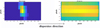 |
Fig. 3 Flux distribution of the direct image and the uncontaminated spectrogram of an object. |
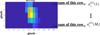 |
Fig. 4 Mixing coefficient estimation from direct images. |
3.1.2 Source matrix estimation
A first solution to estimate the source matrix E is to minimize the following criterion, where ||.||2 is the Frobenius norm
 (27)
(27)
which leads to a least squares (LSQ) estimation:
 (28)
(28)
A second solution for estimating E is to use the least squares with non-negativity constraint (LSQN) algorithm presented in (Lawson & Hanson 1974). Since the spectra to be estimated are by definition non-negative, this method takes this non-negativity into account by minimizing the criterion:
 (29)
(29)
where E ≥ 0 means that all values of the matrix E are nonnegative. Finally, the convolved version of the spectrum of the object of interest, denoted ê1, is the first row of the estimated matrix Ê.
Unlike the first two methods, which require both the direct image of the object of interest and all its contaminants, our third method requires only the image of the object of interest to estimate its spectrum. In fact, this image allows us to estimate the mixing coefficients  of the object of interest in all dispersion directions, which will allow us to estimate the mixing vector as of this object by the same procedure as that described in Sect. 3.1.1. This vector can then be used by a beamforming method to estimate the vector ê1. The goal of the beamformer is to extract a desired signal (spectrum of the object of interest) while attenuating interferences (spectra of contaminants) and noise (Capon 1969; Van Trees 2002). In this paper, we used the beamformer known as the Minimum Power Distortionless Response (MPDR). This beamformer aims to estimate an optimal filter denoted wMPDR, whose output minimizes the total power under the constraint wH as. Assuming that the spectrum of the object of interest is uncorrelated with the spectra of the contaminants, the desired filter is the solution to the following minimization problem,
 (30)
(30)
which leads to the following beamforming coefficients (Van Trees 2002)
 (31)
(31)
where RX = (X - mean(X))(X - mean(X))H/K is the covariance matrix of the observations, mean(X) is the mean over all rows of the matrix X, and K is the number of spectral bands.
Finally, the vector ê1 is estimated as
 (32)
(32)
Although MPDR beamforming can be applied directly to the total observation matrix X to estimate the spectrum of the object of interest, we propose here to split the total observation matrix X into L distinct parts. Each part, denoted Xl, includes all rows of the matrix X and a specific set of columns of this matrix. We then decontaminate each part separately. The goal of this approach is to minimize the risk of encountering underdetermined cases that MPDR beamforming cannot effectively handle. This is because each contaminating object generally contaminates only a portion of the spectrogram of the object of interest. Consequently, the number of contaminants for each of the L parts is less than the number of contaminants for the entire spectrum. To implement this method, we generate L beamformers, each given by
![Mathematical equation: {\bf w}_{\small \text{MPDR}}^{(l)}=\frac{{\bf R}_{{\bf X}_l}^{-1}{\bf a}_s}{{\bf a}_s^H{\bf R}_{{\bf X}_l}^{-1}{\bf a}_s},\hspace*{0.3cm} l\in \left[1,L\right],](/articles/aa/full_html/2026/02/aa57144-25/aa57144-25-eq53.png) (33)
(33)
where RXl is the covariance matrix associated with the l-th part of the observation matrix X. Finally, the outputs  of each beamformer are concatenated to obtain the final estimate of the vector ê1 as follows
![Mathematical equation: \hat{{\bf e}}_{1}=[\hat{{\bf e}}_{1}^{(1)},\hat{{\bf e}}_{1}^{(2)},...,\hat{{\bf e}}_{1}^{(L)}].](/articles/aa/full_html/2026/02/aa57144-25/aa57144-25-eq55.png) (34)
(34)
We note that this method also attenuates unmodeled interferences, such as the spectra of undetected objects or hot pixels, which should lead to better results under these conditions. Knowing that each column of the mixing matrix A is estimated up to a scaling coefficient, the three local instantaneous methods proposed in this section estimate ê1 up to a scaling factor.
3.2 Local convolutive method
Unlike the approach presented in Sect. 3.1, which is based on an approximate linear instantaneous model, the local convolutive approach is based on a more realistic convolutive mixing model introduced in Sect. 2.3. This model allows for a simultaneous decontamination and deconvolution of spectra.
3.2.1 Mixing matrix estimation
We recall the definition of the direct image  , as given in Eq. (26), for an astronomical object with an index, j, in the dispersion direction, di :
 (35)
(35)
By computing the 2D Fourier transform in the spatial domain and assuming that the direct image  is centered with respect to the position of the object of interest in the two spatial dimensions x and y, we obtain
 (36)
(36)
where  is the 2D Fourier transform of
  and
and  is a constant independent of the spatial frequencies fx and fy. Consequently, the mixing coefficients
  in the Fourier domain corresponding to a given object of index j (target or contaminant), can be estimated up to factors Cj using direct images for each dispersion direction. This allows us to estimate the total mixing matrix A(fx) defined in (24).
However, before estimating the mixing coefficients  using the direct images, some preprocessing is required. Firstly, it is essential to align the direct image of each object with the spectrogram of the object of interest in both spatial dimensions, x and y, which is a necessary condition for the validity of Eq. (36). Secondly, it is necessary to correct the photometric PSF by convolving it with the differential PSF between Euclid ’s photometer and spectrometer. Thirdly, it is necessary to normalize the Fourier transform of each image to avoid the introduction of scaling factors.
Once these preprocessings are completed, the mixing vectors of the object of interest  can be estimated using the direct images
  of the object of interest, and the contaminant mixing matrices
  can be estimated using the direct images of the contaminants
  . The total mixing matrix A(fx) defined in (24) is then constructed using the calculated matrices
  and the vectors
  .
.
The procedure for estimating the mixing matrix at each horizontal frequency fx is presented in Algorithm 1.
3.2.2 Source matrix estimation
After constructing the mixing matrix A(fx) for each horizontal frequency fx, the next step is to estimate the source matrix S(fx). However, the mixing matrix A is often underdetermined (i.e. M < N), making it noninvertible. To solve this problem, we have assumed the following two realistic assumptions:
At most Nc (Nc ≤ M - 1) contaminants are active at each horizontal frequency fx;
The source of interest is active at all horizontal frequencies fx.
Input: Direct images  of all objects in all directions
  .
.
Result: Mixing matrix A(fx)
1 for di ={0°, 180°, 184°, −4° do
2 Align the image  with the spectrogram of the object of interest
3 Convolve the image  with the differential PSF
4 Compute the 2D Fourier transform in the spatial domain of the image 
5 Normalize the Fourier transform of the image 
6 Construct the mixing vector of the object of interest 
7 for j = 2 to Ni do
8 Align the image  with the spectrogram of the object of interest
9 Convolve the image  with the differential PSF
10 Compute the 2D Fourier transform in the spatial domain of the image 
11 Normalize the Fourier transform of each image 
12 end
13 construct 
14 end
15 return A(fx)
Next, the procedure for detecting the indices of the Nc contaminants active in each horizontal frequency, fx, is presented in the algorithm 2, which can be seen as a modified version of the Orthogonal Matching Pursuit (OMP) algorithm (Pati et al. 1993; Tropp & Gilbert 2007). In the algorithm 2, H denotes the Hermitian transpose, ind(fx) is the vector of indices related to the object of interest and the dominant contaminants, A(:, ind(fx)) represents a submatrix of A(fx) with all the rows and only the columns present in the vector ind( fx) at the horizontal frequency fx, and pinv is the pseudo-inverse of a matrix, defined by pinv(M) = (MHM)−1MH. The algorithm returns an index vector ind(fx) indicating which contaminants are detected in each horizontal frequency fx. It works by initializing a residual r, then iterates to find the contaminant indices one by one by maximizing the correlation between the residual r and the different columns of the matrix A(fx). Once a contaminant is detected, it is removed from the residue, and the process continues until all Nc contaminants have been identified.
Input: Mixing matrix A(fx), observation vector X(fx) and the assumed number of active contaminants Nc.
Result: Index vector ind(fx)
1 Initialization: ind(fx)=[1], r = X(fx)-A(:,ind(fx))(pinv(A(:,ind(fx)))X(fx))
2 for i = 1 to Nc do
3 Find the index i that maximizes |AH(:,i)r|
4 Set ind(fx)=[ind(fx), i]
5 Set r = X(fx)-A(:,ind(fx))(pinv(A(:,ind(fx)))X(fx))
6 end
7 return ind(fx)
Once the vector ind(fx) is estimated, we propose to use a beamforming technique to estimate the Fourier transform of the spectrum of the object of interest. In our method, we used the beamformer called Linearly Constrained Minimum Power (LCMP) (Tian et al. 2001). This beamformer aims to estimate an optimal filter denoted by wLCMP(fx) at each horizontal frequency fx, whose output minimizes the total power under the constraint wH(fx)A(:, ind(fx)) = [1,0,..., 0]. The filter we are looking for is the solution to the following minimization problem (Tian et al. 2001):
![Mathematical equation: \begin{split} {\bf w}_{\small \text{LCMP}} (f_x)=&\operatorname*{argmin}_{{\bf w}(f_x)}\:\left\{{\bf w}^{\rm H} (f_x){\bf R}_{\bf X}{\bf w}(f_x)\right\},\\ &\text{such that}\,\,\, \ {\bf w }^{\rm H} (f_x){\bf A}(:,\boldsymbol{{ind}}(f_x))=[1, 0, \cdots, 0], \end{split}](/articles/aa/full_html/2026/02/aa57144-25/aa57144-25-eq83.png) (37)
(37)
which leads to the following beamforming coefficients,
 (38)
(38)
where RX = (X - mean(X))(X - mean(X))H/Nf is an estimate of the covariance matrix of the observations, X = [X(1) ∙∙∙ , X(Nf)] is a matrix combining the observation vectors for all frequencies, Nf is the number of horizontal frequencies, and g = [1,0, ∙∙∙, 0]T.
Next, a compressed version of the Fourier transform of the spectrum of the object of interest, S1, is estimated as4
 (39)
(39)
Finally, the spectrum of the object of interest is obtained by applying the Inverse Fourier Transform (IFT) to the signals S1 as follows
 (40)
(40)
For clarity, we use the acronyms LI-LSQ (Linear Instantaneous LSQ), LI-LSQN (Linear Instantaneous LSQN), LI-MPDR (Linear Instantaneous MPDR), and LC-LCMP (Linear Convo-lutive LCMP) to refer to the different methods proposed in this section.
4 Test results
In this section, we evaluate the decontamination performance of the methods proposed in this paper through four different experiments. The first three experiments aim to evaluate the decontamination performance on three different scenarios, each representing a different level of contamination. The fourth experiment evaluates these performances on a set of 100 different objects. These evaluations were performed using realistic, noisy Euclid-like simulations from the SC8 R11 release, provided by the Euclid Consortium. It is important to note that the observed data are also affected by high levels of noise introduced by the acquisition instruments.
4.1 Performance measurement criteria
To measure decontamination performance, we use three main criteria. The first criterion, called SIRimp, evaluates the improvement in the Signal to Interference Ratio (SIR) before and after decontamination. It is defined as the difference between SIRout and SIRin, expressed as
 (41)
(41)
where
 (42)
(42)
where  is the 1D spectrum of the observed data (obtained by averaging all the rows of the observed spectrogram) in the di direction, Ss is the true noiseless spectrum of the object of interest, and Ss is its estimate obtained using a decontamination method. In (42), all spectra are centered and Ŝs and
  are normalized to have the same variance as Ss.
The second criterion called the root mean square error (RMSE) is defined as
 (43)
(43)
The third criterion, called the local RMSE (LRMSE), measures the estimation error within a small region centered around the true position of the main emission line. It is defined as
 (44)
(44)
where L denotes a set of KL wavelength indices corresponding to a small region around the true position of the main emission line of the object of interest. In all tests, KL is set to 20.
It is important to note that SIRimp evaluates the improvement provided by the methods before and after decontamination in terms of interference reduction (mainly contaminant spectra), whereas RMSE simply evaluates the estimation error after decontamination and LRMSE specifically focuses on the estimation error around the main emission line. Better performance is indicated by a higher value of SIRimp and lower values of RMSE and LRMSE.
4.2 Simple scenario without hot pixels
In our first experiment, we chose a simple scenario where the spectrogram of an object of interest (a star-forming galaxy with a redshift of 1.12) is slightly contaminated in all four dispersion directions. The observed spectrograms and corresponding 1D spectra5 for this object are shown in Fig. 5.
The true noiseless spectrum of the object of interest and its estimates using our methods LI-LSQ, LI-LSQN, LI-MPDR and LC-LCMP after normalization by their maximum are shown in Fig. 6. Numerical results in terms of SIRimp, RMSE and LRMSE for this scenario are presented in Table 1.
Fig. 6 clearly demonstrates the efficiency of the proposed methods for decontaminating the spectrum of the object of interest in this first scenario. Indeed, all methods successfully attenuate the contamination from other objects in this scenario. It should be noted that the estimated spectra are noisy, which is to be expected given the high level of noise in the observed data and the fact that our methods aim at separating sources rather than denoising them. The results presented in Table 1 confirm this conclusion. It can be observed that the RMSE and LRMSE values for all methods are low, and the SIRimp values are high, indicating their effectiveness in removing contaminants. Finally, it can be seen that our LC-LCMP method yields the best results for this scenario.
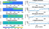 |
Fig. 5 Observed spectrograms (left) and corresponding 1D spectra (right) for the first scenario. |
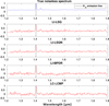 |
Fig. 6 True noiseless spectrum of the object of interest (in blue) and its estimates obtained using the proposed methods (in red) for the first scenario. |
SIRimp in decibel (dB), RMSE and LRMSE obtained for the first scenario.
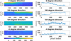 |
Fig. 7 Observed spectrograms (left) and corresponding 1D spectra (right) for the second scenario. |
4.3 Scenario with a few hot pixels
In our second experiment, we chose a complicated scenario where the spectrogram of an object of interest (a star-forming galaxy with a redshift of 0.93) is highly contaminated in all four directions of dispersion. In addition, there are a few hot pixels6 in the −4 degree dispersion direction. The observed spectrograms and corresponding 1D spectra for this object are shown in Fig. 7.
Fig. 8 shows the true noiseless spectrum of the object of interest, along with its estimates using our methods LI-LSQ, LI-LSQN, LI-MPDR and LC-LCMP after normalization by their maximum. This figure clearly demonstrates the efficiency of the proposed methods for decontaminating the spectrum of the object of interest in this scenario. Indeed, all of the proposed methods were successful in eliminating contamination from other objects and hot pixels, and in recovering the main emission line.
The numerical results in terms of SIRimp, RMSE and LRMSE for this scenario are presented in Table 2. This table clearly demonstrates that the LC-LCMP method is the most effective for decontaminating the spectrum of the object of interest in this scenario. Indeed, it outperforms the LI-LSQ, LI-LSQN and LI-MPDR methods by 6.10 dB, 4.64 dB and 2.45 dB respectively in terms of SIRimp. Moreover, the RMSE and the LRMSE of the LC-LCMP method are lower than those of all the other methods.
4.4 Difficult scenario with many hot pixels
In our third experiment, we chose a difficult scenario where the spectrogram of an object of interest (a star-forming galaxy with a redshift of 1.12) is highly contaminated in all four dispersion directions. Additionally, there is at least one hot pixel present in each dispersion direction, further complicating this scenario. The observed spectrograms and corresponding 1D spectra for this object are presented in Fig. 9, where the isolated peaks in the observed 1D spectra are due to hot pixels. Given that the true position of the main Hα emission line is around the wavelength with index 145, it cannot be distinguished in the spectra of Fig. 9 due to the strong contribution of noise and contaminants.
Fig. 10 shows the true noiseless spectrum of the object of interest and its estimates using the above methods after normalization by their maximum. This figure clearly demonstrates the efficiency of the proposed methods LI-MPDR and LC-LCMP for decontaminating the spectrum of the object of interest in this challenging scenario. This result is expected because these two methods use beamforming techniques, which should perform better in the presence of unmodeled interferences such as hot pixels.
Table 3 clearly demonstrates that the LC-LCMP method is the most effective for decontaminating the spectrum of the object of interest in this scenario. Indeed, it outperforms the LI-LSQ, LI-LSQN and LI-MPDR methods by 6.48 dB, 5.75 dB and 1.59 dB respectively in terms of SIRimp. Moreover, the RMSE and the LRMSE of the LC-LCMP method are lower than those of all other methods, validating the effectiveness of this method in this third scenario.
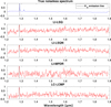 |
Fig. 8 True noiseless spectrum of the object of interest (in blue) and its estimates obtained using the proposed methods (in red) for the second scenario. |
SIRimp (dB), RMSE and LRMSE obtained for the second scenario.
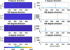 |
Fig. 9 Observed spectrograms (left) and corresponding 1D spectra (right) for the third scenario. |
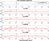 |
Fig. 10 True noiseless spectrum of the object of interest (in blue) and its estimates obtained using the proposed methods (in red) for the third scenario. |
SIRimp (dB), RMSE and LRMSE obtained for the third scenario.
4.5 Performance using 100 objects
To confirm the effectiveness of the proposed methods, we performed the same tests on a total of 100 different objects. The chosen objects for these tests have a redshift 0.9 < z < 1.8, an Hα flux greater than 10−16 erg/s/cm2 and a magnitude varying between 20 and 23.5 AB mag. For the comparison, we used the NMF Alternating Least Square (ALS) method (NMF-ALS) described in Paatero & Tapper (1994).
The NMF-ALS method is a BSS method based on source positivity. It involves finding an approximate decomposition of the total observation matrix X, as defined in (14), into two non-negative matrices, with the aim of identifying one of these matrices as the mixing matrix A and the other as the source matrix E. This method uses only the observation matrix X and does not utilize any additional available information, such as direct images. The primary limitation with the NMF-ALS method is the nonuniqueness of its solutions (Paatero & Tapper 1994). Indeed, this iterative approach may converge to the desired solution (A, E), but it can also converge to a different (local) minimum that deviates from this solution.
The results, in terms of the averages of SIRimp (dB), RMSE and LRMSE as well as their respective standard deviations, are presented in Table 4.
Table 4 clearly demonstrates that the LC-LCMP method outperforms all other methods in terms of average SIRimp (dB), RMSE and LRMSE. Indeed, this method shows average SIRimp improvements of 2.67 dB, 2.37 dB, 1.39 dB and 8.59 dB compared to the LI-LSQ, LI-LSQN, LI-MPDR and NMF-ALS methods, respectively. The superiority of the LC-LCMP method in terms of SIRimp can be explained by the fact that the convolu-tive mixing model used by this method is more accurate than the approximate linear instantaneous model presented in Sect. 2.2 and used by the other methods. The mean LRMSE of the LC-LCMP method is again lower than that of all other methods. This result is expected and can be explained by the fact that the LC-LCMP method aims to estimate deconvolved versions of the spectra, providing more accurate estimates around the main emission line. In contrast, all other methods provide sources convolved by a function that depends on the object profile in the dispersion direction, which consequently impairs the accuracy of the estimate in the region around the main emission line. Moreover, the mean RMSE of the LC-LCMP method is lower than that of all other methods, validating the effectiveness of this method.
In terms of standard deviations, the NMF-ALS method has a significantly lower SIRimp standard deviation than the others. The reason for this result is that this method typically produces consistently poor results, which do not vary significantly from one experiment to another when compared to the proposed methods. It is important to highlight that the LI-LSQ method exhibits the lowest standard deviation in terms of SIRimp among all the proposed methods, while the LI-LSQN method has the lowest standard deviation in terms of RMSE, and the LC-LCMP method shows the lowest standard deviation in terms of LRMSE.
Next, we examine the behavior of our methods as a function of object magnitude and Hα flux, using these 100 objects. Figs. 11 and 12 show the performance obtained in this experiment in terms of SIRimp, RMSE and LRMSE.
Fig. 11 shows that the performance of our methods in terms of SIRimp remains relatively stable as a function of the magnitude of the objects to be decontaminated. Regarding the performance of the methods in terms of RMSE and LRMSE, we generally observe that for all the methods, an increase in the magnitude of the objects to be decontaminated leads to higher RMSE and LRMSE values. This is to be expected, as the lower the brightness of an object, the more challenging it is to decontaminate it due to the increased number of contaminants that are brighter than the object. Fig. 12 shows that a decrease in the Hα flux of the objects to be decontaminated results in a corresponding decrease in the performance of our methods in terms of SIRimp, RMSE, and LRMSE.
For all the proposed methods except for LI-MPDR, the computation time varies depending on the number of contaminants and treated objects. The LI-MPDR method offers the best performance in terms of computation time. In fact, its computation time is almost half that of the LI-LSQ, LI-LSQN, and LC-LCMP methods.
Means and standard deviations of SIRimp (dB), RMSE and LRMSE using 100 objects.
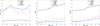 |
Fig. 11 Performance of the methods as a function of magnitude. |
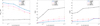 |
Fig. 12 Performance of the methods as a function of Hα flux. |
5 Conclusion and perspectives
In this paper, we propose four new separation methods adapted to Euclid-like spectra that are based on two different local approaches. The first approach is called the local instantaneous approach, which uses an approximate instantaneous model. The second approach is called the local convolutive approach, which uses a more realistic convolutive model. For each approach, we developed a mixing model that links the observed data to the source spectra, simultaneously taking into account four grism dispersion directions, either in the spatial domain for the instantaneous approach or in the Fourier domain for the convolutive approach. We then developed several methods for decontaminating these spectra from mixtures, exploiting the direct images provided by the NIR photometers. The test results presented in Sect. 4 confirm the effectiveness of all the proposed methods. In particular, the local convolutive method performs remarkably well in terms of SIRimp, RMSE, and LRMSE, clearly outperforming other methods based on a linear instantaneous mixing model.
In terms of perspectives, it would be interesting to apply the proposed methods to real Euclid satellite data when they become available. Additionally, it could be beneficial to replace the local approach used by all the methods proposed in this article, where decontamination is carried out object by object, with a global approach where all objects located in a predefined zone are decontaminated simultaneously. In addition, in our work, we have exploited direct images of the spectral band J to obtain an estimate of the mixing coefficients. When direct images of the other bands Y and H become available, they can also be exploited to improve our estimate of the mixing coefficients. Finally, in the proposed models, we have assumed that the PSF is spectrally invariant, whereas this PSF varies slightly as a function of wavelength. Taking this variation into account could improve the accuracy of the proposed models.
Acknowledgements
The authors thank their colleagues from the SIR and SIM organizational units of the Euclid project. The SIM team provided the essential simulated data used in this work, and the SIR team performed the crucial data preprocessing steps. Their contributions were foundational to this work.
References
- Bella, M., Hosseini, S., Saylani, H., et al. 2022a, in 30th European Signal Processing Conference (EUSIPCO), 1981 [Google Scholar]
- Bella, M., Saylani, H., Hosseini, S., & Deville, Y. 2022b, in International Workshop on Multimedia Signal Processing 2022 (MMSP 2022), 741 [Google Scholar]
- Bella, M., Saylani, H., Hosseini, S., & Deville, Y. 2023, IEEE Access, 11, 100632 [Google Scholar]
- Bella, M., Hosseini, S., Saylani, H., Grégoire, T., & Deville, Y. 2024, in IEEE International Conference on Acoustics, Speech, and Signal Processing (ICASSP 2024), 5995 [Google Scholar]
- Bioucas-Dias, J. M., Plaza, A., Dobigeon, N., et al. 2012, IEEEJ. Sel. Top. Appi. Earth Obs. Remote Sens., 5, 354 [Google Scholar]
- Brammer, G. 2019, Astrophysics Source Code Library [record ascl:1905.001] [Google Scholar]
- Capon, J. 1969, Proc. IEEE, 57, 1408 [CrossRef] [Google Scholar]
- Comon, P. 1994, Signal Process., 36, 287 [CrossRef] [Google Scholar]
- Comon, P., & Jutten, C. 2010, Handbook of Blind Source Separation: Independent Component Analysis and Applications (Oxford: Academic Press) [Google Scholar]
- Costille, A., Caillat, A., Rossin, C., et al. 2019, in International Conference on Space Optics-ICSO 2018, 11180, 418 [Google Scholar]
- Deville, Y. 2016, Blind Source Separation and Blind Mixture Identification Methods (John Wiley & Sons, Ltd), 1 [Google Scholar]
- Dokkum, P. V., & Pasha, I. 2024, PASP, 136, 034503 [Google Scholar]
- Euclid Collaboration (Scaramella, R., et al.) 2022, A&A, 662, A112 [NASA ADS] [CrossRef] [EDP Sciences] [Google Scholar]
- Euclid Collaboration (Jahnke, K., et al.) 2025, A&A, 697, A3 [Google Scholar]
- Euclid Collaboration (Mellier, Y., et al.) 2025, A&A, 697, A1 [Google Scholar]
- Freudling, W., Kümmel, M., Haase, J., et al. 2008, A&A, 490, 1165 [NASA ADS] [CrossRef] [EDP Sciences] [Google Scholar]
- Gardner, J. P., Mather, J. C., Abbott, R., et al. 2023, PASP, 135, 068001 [NASA ADS] [CrossRef] [Google Scholar]
- Gribonval, R., & Lesage, S. 2006, in ESANN’06 proceedings-14th European Symposium on Artificial Neural Networks (d-side publication), 323 [Google Scholar]
- Heylen, R., Parente, M., & Gader, P. 2014, IEEE J. Sel. Top. Appl. Earth Obs. Remote Sens., 7, 1844 [Google Scholar]
- Hosseini, S., Selloum, A., Contini, T., & Deville, Y. 2020, Digit. Signal Process., 106, 102837 [Google Scholar]
- Hyvärinen, A., & Oja, E. 2000, Neural Netw., 13, 411 [CrossRef] [Google Scholar]
- Igual, J., & Llinares, R. 2007, Digit. Signal Process., 17, 947 [Google Scholar]
- Kümmel, M., Walsh, J., Pirzkal, N., Kuntschner, H., & Pasquali, A. 2009, PASP, 121, 59 [CrossRef] [Google Scholar]
- Laureijs, R., Amiaux, J., Arduini, S., et al. 2011, ESA/SRE(2011)12 [arXiv:1110.3193] [Google Scholar]
- Lawson, R. J., & Hanson, C. L. 1974, Solving Least Squares Problems (Englewood Cliffs: Prentice-Hall) [Google Scholar]
- Lee, D. D., & Seung, H. S. 1999, Nature, 401, 788 [Google Scholar]
- Makino, S. 2018, Audio Source Separation, 433 (Springer) [Google Scholar]
- Markovic, K., Percival, W. J., Scodeggio, M., et al. 2017, Mon. Not. R. Astron. Soc., 467, 3677 [Google Scholar]
- Meganem, T., Hosseini, S., & Deville, Y. 2015, in Non-negative Matrix Factorization Techniques: Advances in Theory and Applications (Springer), 133 [Google Scholar]
- Momcheva, I. G., Brammer, G. B., Van Dokkum, P. G., et al. 2016, Astrophys. J. Suppl. Ser., 225, 27 [Google Scholar]
- O’grady, P., Pearlmutter, B., & Rickard, S. 2005, Int. J. Imaging Syst. Technol., 15, 18 [Google Scholar]
- Paatero, P., & Tapper, U. 1994, Environmetrics, 5, 111 [Google Scholar]
- Palmer, C., & Loewen, E. G. 2005, Diffraction Grating Handbook (New York: Newport Corporation) [Google Scholar]
- Pati, Y., Rezaiifar, R., & Krishnaprasad, P. 1993, in Proceedings of 27th Asilomar Conference on Signals, Systems and Computers, 1, 40 [Google Scholar]
- Ryan, R., N., S. C., & Pirzkal. 2018, PASP, 130, 034501 [CrossRef] [Google Scholar]
- Schirmer, M., Jahnke, K., Aussel, G. S. H., et al. 2022, A&A, 662, A92 [NASA ADS] [CrossRef] [EDP Sciences] [Google Scholar]
- Selloum, A., Hosseini, S., Deville, Y., & Contini, T. 2015, in 2015 23rd European Signal Processing Conference (EUSIPCO), 1641 [Google Scholar]
- Selloum, A., Hosseini, S., Deville, Y., & Contini, T. 2016, in 2016 IEEE 26th International Workshop on Machine Learning for Signal Processing (MLSP), 1 [Google Scholar]
- Tian, Z., Bell, K. L., & Trees, H. V. 2001, IEEE Trans. Signal Process., 49, 1138 [Google Scholar]
- Tropp, J. A., & Gilbert, A. C. 2007, IEEE Trans. Inf. Theory, 53, 4655 [CrossRef] [Google Scholar]
- Van Trees, H. L. 2002, in Optimum Array Processing (John Wiley and Sons, Ltd), 710 [Google Scholar]
- Zarzoso, V., & Nandi, A. K. 2001, IEEE Trans. Biomed. Eng., 48, 12 [Google Scholar]
- Zokay, M., & Saylani, H. 2022, in Annual Conference on Medical Image Understanding and Analysis (Springer), 734 [Google Scholar]
In practice, the PSF varies slightly with wavelength. However, this variation is not considered in this work.
It should be noted that, even if Eq. (4) is obtained for dispersion in the horizontal direction x, it remains valid for all dispersion directions di ∈ 0°, 180°, 184°, −4° after rotating the spectrograms for each direction according to their respective angles.
By simultaneously using the three direct NISP images in the Y, J and H bands, we can reduce this estimation error. However, during our work, we only had access to the image in the J band.
Note that the relations (38) and (39) are applied for each horizontal frequency fx.
The observed 1D spectrum is defined here as the average of all rows in the spectrogram.
A hot pixel is a pixel in the spectrogram that has a very high magnitude relative to neighboring pixels. These hot pixels are often the result of defects at this pixel in the detector (Dokkum & Pasha 2024).
All Tables
All Figures
|
Fig. 1 Contamination of the spectra of neighboring objects at the output of the grism. |
| In the text | |
|
Fig. 2 Euclid ’s observation strategy. |
| In the text | |
|
Fig. 3 Flux distribution of the direct image and the uncontaminated spectrogram of an object. |
| In the text | |
|
Fig. 4 Mixing coefficient estimation from direct images. |
| In the text | |
|
Fig. 5 Observed spectrograms (left) and corresponding 1D spectra (right) for the first scenario. |
| In the text | |
|
Fig. 6 True noiseless spectrum of the object of interest (in blue) and its estimates obtained using the proposed methods (in red) for the first scenario. |
| In the text | |
|
Fig. 7 Observed spectrograms (left) and corresponding 1D spectra (right) for the second scenario. |
| In the text | |
|
Fig. 8 True noiseless spectrum of the object of interest (in blue) and its estimates obtained using the proposed methods (in red) for the second scenario. |
| In the text | |
|
Fig. 9 Observed spectrograms (left) and corresponding 1D spectra (right) for the third scenario. |
| In the text | |
|
Fig. 10 True noiseless spectrum of the object of interest (in blue) and its estimates obtained using the proposed methods (in red) for the third scenario. |
| In the text | |
|
Fig. 11 Performance of the methods as a function of magnitude. |
| In the text | |
|
Fig. 12 Performance of the methods as a function of Hα flux. |
| In the text | |
Current usage metrics show cumulative count of Article Views (full-text article views including HTML views, PDF and ePub downloads, according to the available data) and Abstracts Views on Vision4Press platform.
Data correspond to usage on the plateform after 2015. The current usage metrics is available 48-96 hours after online publication and is updated daily on week days.
Initial download of the metrics may take a while.