| Issue |
A&A
Volume 706, February 2026
|
|
|---|---|---|
| Article Number | A120 | |
| Number of page(s) | 7 | |
| Section | Atomic, molecular, and nuclear data | |
| DOI | https://doi.org/10.1051/0004-6361/202557443 | |
| Published online | 05 February 2026 | |
Calculated oscillator strengths and transition probabilities of singly ionised nickel (Ni II)
1
Physics Department, Imperial College London,
London
SW7 2AZ,
UK
2
Anton Pannekoek Institute for Astronomy (API), University of Amsterdam,
Science Park 904,
1098
XH
Amsterdam,
The Netherlands
3
Space Research Organisation Netherlands (SRON),
Niels Bohrweg 4,
2333
CA
Leiden,
The Netherlands
★ Corresponding author: This email address is being protected from spambots. You need JavaScript enabled to view it.
Received:
26
September
2025
Accepted:
25
December
2025
Abstract
Aims. This work reports calculated transition probabilities for spectral lines of singly ionised nickel (Ni II) incorporating newly determined experimental energy levels, addressing critical gaps in atomic data required for astrophysical spectroscopy and plasma diagnostics.
Methods. Transition probabilities of Ni II were calculated using the semi-empirical orthogonal operator method for both odd and even energy levels. Calculated eigenvalues were fine-tuned to experimental energy levels, determined using Fourier transform spectroscopy, further increasing the accuracy of these calculated transition probabilities.
Results. In total, transition probabilities have been calculated for nearly 118 000 electric dipole transitions between 361 even and 735 odd levels. The resulting transition probabilities show strong agreement with existing experimental and semi-empirical data, while offering improved consistency and coverage across a wide range of line strengths. The calculated transitions span the far-infrared to the vacuum ultraviolet spectral regions, providing extensive coverage for astrophysical applications. This dataset significantly enhances the calculated atomic data available for Ni II and represents a critical contribution to the advancement of our understanding of astrophysical phenomena through improved spectroscopic analysis.
Key words: atomic data / atomic processes
© The Authors 2026
 Open Access article, published by EDP Sciences, under the terms of the Creative Commons Attribution License (https://creativecommons.org/licenses/by/4.0), which permits unrestricted use, distribution, and reproduction in any medium, provided the original work is properly cited.
This article is published in open access under the Subscribe to Open model. This email address is being protected from spambots. You need JavaScript enabled to view it. to support open access publication.
1 Introduction
Accurate atomic data are of paramount importance for astrophysics, underpinning the interpretation of spectral lines and enabling insights into the physical and chemical conditions of astrophysical plasmas. In particular, transition probabilities enable the determination of elemental abundances and form key inputs into stellar atmospheric models, enabling the study of stellar and galactic formation and evolution. Without precise transition probabilities, the ability to extract meaningful information from astronomical observations is significantly limited. In this study, we present new semi-empirical transition probabilities for singly ionised nickel (Ni II), calculated using the orthogonal operator method and calibrated against newly determined energy levels from high-resolution Fourier transform spectroscopy (FTS).
Iron-group elements play a crucial role in the composition of spectra of various astronomical objects due to their high relative cosmic abundance and complex spectral features. These elements significantly influence the observed spectra of the Sun, stars, the interstellar medium and quasi-stellar objects among many others. The dominance of the singly ionised iron group elements is particularly pronounced in many B- to G-type stars, where accurate atomic data are essential for reliable spectral analysis. As the second most abundant iron group element, there is an on-going and acute demand for accurate atomic data of Ni II and there have been a number of experimental, observational and theoretical works during the past five decades aimed at improving the quantity and quality of available transition probability data for this important species.
Experimental transition probabilities for electric dipole transitions of a small number of Ni II lines have been measured using a number of techniques. Fedchak & Lawler (1999) presented radiative lifetimes for 18 odd-parity levels of Ni II, measured using time-resolved laser-induced fluorescence (TR-LIF). These measurements were combined with emission branching fractions measured using Fourier transform and grating spectrometers to produce 59 absolute transition probabilities in the ultraviolet (UV) and vacuum ultraviolet (VUV) regions, with a typical uncertainty of ~10%. Fedchak et al. (2000) expanded on this work by measuring relative absorption oscillator strengths for six resonance lines in the VUV which were then normalised to absolute values using three A-values from the previous study of Fedchak & Lawler (1999).
Manrique et al. (2011) used laser-induced breakdown spectroscopy (LIBS) to measure transition probabilities for 19 Ni II spectral lines. The technique employed a laser for ablation and ionisation, followed by a fast, time-resolved spectrometer for capturing the emission spectra. They estimated their uncertainties to be 15%. Manrique et al. (2013) revisited the use of LIBS, measuring transition probabilities for 48 Ni II spectral lines, with an uncertainty of 13%. Their values agreed well with the previous measurements of Fedchak & Lawler (1999) and had satisfactory agreement with theoretical calculations for the 17 newly measured lines.
Hartman et al. (2017) measured radiative lifetimes of seven high-lying 3d84d Ni II levels using TR-LIF. These experimental lifetimes, along with lifetimes and branching fractions calculated using a pseudo-relativistic Hartree–Fock method, were used to derive 477 semi-empirical transition probabilities for Ni II. The resulting log(gf) values were on average 20% higher than previous calculations, with calculated lifetimes agreeing within 5% of the experimental values.
While experimental data are always preferred for highresolution spectral analyses, theoretical calculations remain essential for extending coverage to transitions inaccessible to laboratory measurements. Early theoretical investigations into the transition probabilities of Ni II for the low-lying 3d84p to 3d84s lines were conducted by Gruzdev (1962) and Mendlowitz (1966) using intermediate coupling calculations. In the following decades, Kurucz utilised Cowan code calculations (Cowan 1981) to determine atomic data for a large number of elements and ionisations, which culminated in a comprehensive data compilation (Kurucz 2011). These calculated transition probabilities align reasonably well with experimental values in the UV (Fedchak & Lawler 1999), but show significant divergence for resonance lines at shorter wavelengths in the VUV (Fedchak et al. 2000).
Fritzsche et al. (2000) used Multi-Configuration Dirac-Fock wavefunctions generated via the GRASP92 code (Parpia et al. 1996), to calculate transition probabilities using the REOS program (Fritzsche & Anton 2000). Fritzche et al estimated an uncertainty of better than 25% for strong lines based on comparison with previous theoretical and experimental data, but weaker transitions were expected to have much larger uncertainties.
The most recent large-scale, theoretical study of Ni II is from Cassidy et al. (2016) who performed extensive atomic structure calculations using the CIV3 code (Hibbert 1975) to calculate transition probabilities for 5023 electric dipole transitions among the 3d9, 3d84s, 3d74s2, 3d84p and 3d74s4p levels. They determined configuration interaction wavefunctions with relativistic effects incorporated through the Breit-Pauli approximation. Two sets of calculations were performed, with different 3d and 4d functions, to determine the effect of state-to-state variation. The results of the two calculations showed reasonable agreement, showing a plausible level of convergence in the work. However, certain levels exhibited strong configuration interaction mixing, which led to significant differences in the oscillator strengths for transitions involving those levels, highlighting the complexity of calculating accurate transition data, especially in the presence of strong configuration interaction mixing.
In this work, we present new semi-empirical calculations of oscillator strengths for Ni II, performed using the orthogonal operator method. Crucially, these calculations incorporate newly determined experimental energy levels (Clear et al. 2022a, 2023), allowing for fine-tuning of the atomic structure parameters and significantly improving the accuracy of the resulting transition probabilities. These energy levels, obtained via highresolution FTS, are the most precise measurements available. By incorporating these refined energies, atomic structure parameters are carefully adjusted allowing for improved modelling of configuration interaction and transition probabilities. As a result, the oscillator strengths reported here are expected to be the most accurate to date for Ni II, offering a valuable resource for astrophysical applications and a robust benchmark for future experimental and theoretical studies.
2 Orthogonal operator method
The calculation of accurate transition probabilities for atomic systems requires the determination of highly precise eigenvectors. This is particularly critical for complex systems such as the iron group elements, which exhibit dense energy level structures and strong configuration interaction. In such cases, semi-empirical approaches have proven effective in achieving reliable results (Uylings & Raassen 2019). To calculate accurate eigenvectors, and therefore transition probabilities, for Ni II, we have employed the semi-empirical orthogonal operator method. Detailed descriptions of the method are given in Uylings & Raassen (2019) and Uylings (2021), but a brief overview of its application in this study is provided below.
The orthogonal operator method begins with the construction of a model Hamiltonian expressed in terms of orthogonal spin-angular operators. These operators form a mathematically independent basis, allowing each associated radial parameter to be varied, introducing only minimal correlations with others. This independence ensures numerical stability and enables the systematic incorporation of physical effects, including higherorder perturbative and relativistic interactions, which are essential for reducing residual deviations in the fit. The parameters of the Hamiltonian are adjusted via a least-squares optimisation to reproduce experimental energy levels as closely as possible.
For this study, we used 547 recently published experimental energy levels obtained through high-resolution FTS (Clear et al. 2022a, 2023). These measurements represent an order-ofmagnitude improvement in accuracy over previous datasets (e.g. Shenstone 1970), and provide a significantly improved representation of the energy structure of Ni II. This, in turn, enhances the accuracy of our computed eigenvectors and increases the reliability of the resulting transition probabilities.
Despite good agreement between calculated and experimental eigenvalues, inaccuracies in the eigenvectors may still persist. These are typically dominated by magnetic interactions within a configuration, though inter-configuration mixing can also contribute. To minimise such effects, we constructed extended model spaces for both low- and high-lying levels. For the lower levels, the model includes seven even-parity configurations (3d9, 3d84s, 3d74s2, 3d84d, 3d85s, 3d85d, 3d86s) and five odd-parity configurations (3d84p, 3d74s4p, 3d64s24p, 3d85p, 3d84f). The overall mean deviation of the fit is 19 cm−1 for the even system and 82 cm−1 for the odd system, with the lowest three even configurations fitted to within 7.8 cm−1 and the 3d84p system to within 15 cm−1. The lower-lying level system contained 564 odd and 203 even levels.
For higher-lying levels, which predominantly share the 3d8(3F) parent term and exhibit reduced configuration interaction, the model space was extended to include seven even-parity configurations (3d86d, 3d87d, 3d87s, 3d88s, 3d89s, 3d85g, 3d86g) and five odd-parity configurations (3d86p, 3d87p, 3d85f, 3d86f, 3d86h). The resulting fits yielded mean deviations of 8.8 cm−1 for the even system and 25 cm−1 for the odd system, indicating excellent agreement with experimental energies. The higher-lying level system used 171 odd and 158 even levels.
Once the Hamiltonian parameters were optimised, angular coefficients for the transition matrix were computed. These were combined with transition integrals obtained from relativistic Hartree–Fock calculations. The resulting LS-coupled transition matrix was transformed using the fitted eigenvectors, and the squared matrix elements were used to derive line strengths and A-values for all modelled transitions.
As discussed in Section 1, previous calculations of Ni II transition probabilities have relied either on fully ab initio methods or semi-empirical approaches based on less accurate experimental energy levels. By incorporating high-precision experimental energies, an expanded configuration basis, and the systematic flexibility of the orthogonal operator method, the present calculations are expected to yield oscillator strengths of significantly improved accuracy. A detailed comparison with existing datasets is presented in Section 3.2.
The primary benefit of adopting high-precision experimental energy levels lies in the resulting eigenvectors from the orthogonal operator approach. These eigenvectors govern the mixing of configuration state functions and therefore the accuracy of calculated transition probabilities. Whilst the strongest lines, which are typically associated with energy levels of nearly pure LS-coupling, obviously show little sensitivity to improved eigenvector compositions, weaker and intermediate-strength lines, such as intercombination lines, can be significantly affected. These lines are often critical in astrophysical applications such as abundance determinations.
For Ni II, comparison with neighbouring spectra (e.g. Fe II (Raassen & Uylings 1998), Co II (Raassen & Uylings 1998), Cu II (Kramida et al. 2017)), where more extensive experimental data exist, suggests that accuracies for intermediatestrength lines improves from approximately 30–40% (traditional Cowan approach) to around 10–15% using orthogonal operators with high-accuracy level energies. Thus, while improvements for strong transitions from high-purity LS-coupled levels are modest, the enhanced accuracy for intermediate-strength lines represents a substantial gain for astrophysical modelling.
To provide a quantitative illustration for the discussion above, we include a spectral line intensity comparison for a selected set of weak and intermediate-strength Ni II lines. Table A.1 presents results from several approaches. The first seven columns give the air wavelength, energy, label and J value of the even and odd levels of the transition. Columns eight to eleven give the gA results from the following approaches: (8) the present calculation using a 7-even × 5-odd configuration basis with complete orthogonal operators; (9) a modified orthogonal calculation where effective operators for 3d84d and 3d84p were set to zero, placing it between the full orthogonal operator approach and the traditional Cowan method. The gA differences between these calculations highlights the important effect of including these operators. (10) Cowan-based results from Kurucz (Kurucz 2011); and (11) the present calculation with an LTE population distribution for a plasma temperature of 15 000 K (an estimate of plasma discharge source temperature for the experimental line intensities). Column twelve gives the cancellation factor (CF) for the present calculation and experimental line intensities from Shenstone (1970, 1971) and an unpublished grating linelist measured in 2016 by the lead author of this paper are given in columns thirteen and fourteen. Note, the intensities of the two experimental linelists should not be compared with each other directly, as they use different intensity scales.
Whilst most cases show modest gA differences, Table A.1 highlights instances where the omission of effective operators leads to discrepancies of up to two orders of magnitude, demonstrating the importance of using an expanded and systematically optimised parameter set. Practically all lines in the table have very small cancellation factors, reinforcing that large transition probability deviations correlate with strong cancellation and level mixing.
3 Results and discussion
3.1 E1 transition probabilities
Using the method discussed in Section 2, we calculated A-values for electric dipole (E1) transitions of Ni II for the lower-lying and higher-lying systems and these are given in Table A.2. The complete dataset is available as a machine-readable file. Parity-forbidden magnetic dipole (M1) and electric quadrupole (E2) transitions in Ni II are treated separately in Clear et al. (2022b), where new Ritz wavelengths and transition probabilities for astrophysically relevant, parity-forbidden lines were studied. No restrictions were applied to the complete dataset; all calculated transitions are included without limits on log(gf), wavelength, or other selection criteria, allowing the reader to select the data most appropriate for their application.
The first and second columns of Table A.2 give the Ritz wavelength and Ritz wavenumber of the transition respectively, obtained from the difference between the energy level values of the transition. Wavelengths between 200 nm and 2 μm are given as air wavelengths and as vacuum wavelengths for all other transitions. The third, fourth and fifth columns give the J value, energy value and designation of the even level of the transition and columns six, seven and eight repeat this for the odd level. An asterisk after the energy value indicates that the level has an experimental value, otherwise the energy value is the calculated eigenvalue. For transitions involving a calculated eigenvalue, wavelengths and wavenumbers should not be considered spectroscopically accurate. For transitions between purely experimental energy levels, the reader is directed to Clear et al. (2022a, 2023) for Ritz wavelengths and uncertainties. Columns nine and ten give the transition probability (A-value) and log(gf) of the transition. The g value is the statistical weight (2J + 1) of the lower level.
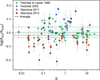 |
Fig. 1 Comparison between the calculated (this work, AOO) and experimental A-values (AEXP) for 3d84p–3d9 and 3d84p–3d84s transitions of Ni II. Error bars show experimental uncertainty only. Solid lines indicate the average log(AOO/AEXP). |
3.2 Comparison with previous data
Following calculation, it is important to assess the accuracy of the new transition probabilities. To this end, we compare our results with existing experimental (EXP) and semi-empirical (SE) datasets. Figures 1 and 2 present comparisons between our calculated A-values and previously published values. In each case, the logarithmic ratio of this work and the published value (log(AOO/AEXP or SE)) is plotted against line strength, S, as both experimental and calculated data have been shown to be more reliable at higher values (Kramida 2013). This approach enables visualisation of systematic offsets and the distribution of residuals across the full range of transition strengths.
3.2.1 Comparison with experimental data: 3d9–3d84p and 3d84s–3d84p transitions
Figure 1 compares our new A-values with purely experimental values for 3d9–3d84p and 3d84s–3d84p transitions, derived from either FTS branching fractions combined with LIF lifetimes (Fedchak & Lawler 1999; Fedchak et al. 2000) or from LIBS measurements (Manrique et al. 2011, 2013). The low scatter in the plot suggests strong internal consistency and supports the conclusion that the orthogonal operator method effectively captures the dominant physical effects governing these transitions.
The main source of uncertainty in the calculation of transition probabilities is commonly the transition integral. Initially, the reduced matrix element ⟨4s∥r1∥4p⟩ = −2.594 au was used in our calculations. This value was calculated from single configuration MCDHF wavefunctions, subsequently reduced by 9% to account for core polarisation effects.
However, fine-tuning of the transition integral led us to adopt a slightly smaller value of −2.353 au for the final calculations, which yielded a better overall agreement with experimental transition probabilities. Table 1 presents a comparison of experimental A-values with those calculated using both transition integrals. The sum of squared residuals is reduced by nearly a factor of four when using the lower transition integral value, indicating improved consistency with measured data. On average, replacing the transition integral of −2.594 au with −2.353 au resulted in an overall reduction in A-values of approximately 82%, as expected from the scaling relation A ∝ |⟨r1⟩|2. Due to configuration mixing, however, this scaling is not exact for individual transitions, and deviations from the expected ratio are observed. The differences between experimental and our calculated values are then smaller than 20%, which seems a reasonable value for the mutual uncertainty of the calculated values for strong lines with S > 2. We estimate uncertainties of 40% for calculated values with line strengths between 0.02 ≤ S ≤ 2 and do not give uncertainty estimates for weaker transitions, where no experimental data are available for comparison.
As an aside, during comparison with experimental A-values, we identified one outlier in Table 1. The A-value of 2.44× 10⁸ s−1 for the λ = 2416.14 Å (3d8(3F)4s2F5/2–3d8(3F)4p2G7/2) transition reported by Manrique et al. (2013) is higher than both our calculations and other experimental data for this transition. We therefore replaced it with the older value of 1.93 × 10⁸ s−1 from Fedchak & Lawler (1999), which aligns more closely with the overall trend of experimental and calculated data. Private correspondence with the authors of Manrique et al. (2011, 2013) suggested two possible reasons for the increased A-value of 2416.14 Å. For the 2013 paper, new Stark widths were used to obtain the centre-of-gravity fits for the spectral lines. Strong lines are very sensitive to Stark widths which would have affected them more than weaker transitions. The second possibility is a failure of the model of a homogeneous plasma used, to which strong lines are again more sensitive than weak ones. Both of these possibilities result in an increased sensitivity of the model and fitting for strong spectral lines like 2416.14 Å in LIBS. Regardless, although we have included the older A-value in our comparison, we do not assert that the A-value published by Manrique et al. (2013) is inaccurate.
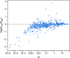 |
Fig. 2 Comparison between calculated (this work, AOO) and semi-empirical A-values (ASE) for 3d84p–3d84d transitions of Ni II (Hartman et al. 2017). Scatter increases noticeably for transitions with line strengths below S = 0.01, reflecting the greater sensitivity of weak transitions to uncertainties in wavefunction composition and transition integrals. This behaviour is consistent with known limitations of transition probability calculations in regions of strong configuration mixing or low transition probability, where small inaccuracies in eigenvectors can lead to disproportionately large errors. |
Comparison of experimental A-values with calculated values using two different reduced matrix elements for the 4s–4p transition. All A-values are in units of 108 s−1.
3.2.2 Comparison with semi-empirical data: 3d84p–3d84d transitions
Figure 2 shows the comparison with transition probabilities for the 3d84p–3d84d transitions derived from experimental lifetimes combined with branching fractions calculated using a pseudorelativistic Hartree–Fock method (Hartman et al. 2017). It is important to note that the vertical scales of Figures 1 and 2 differ significantly.
There is an overall trend for our new A-values to be consistently lower than those reported by Hartman et al. (2017) as transitions become weaker. For lines with S < 0.001, our calculated A-values are consistently smaller than those reported by Hartman et al. Virtually the same reduced matrix elements ⟨4d∥r1∥4p⟩ are used in both studies: 4.557 au by Hartman et al. vs. 4.578 au in the present work. The discrepancy therefore likely arises from differences in eigenvector composition. Given the low standard deviations in our fits to experimental energy levels, we expect that the eigenvectors obtained via the orthogonal operator method are slightly more accurate, particularly in regions of strong configuration mixing.
Table A.1 of Hartman et al. (2017) also presents the cancellation factors (CFs) as defined by Cowan (Cowan 1981). Nearly all outlier transitions in Figure 2, those with log(AOO/ASE) > 1 or < −1.5, are associated with CFs below 0.04 in Hartman et al. (2017). As highlighted by Hartman et al., transitions with CF < 0.05 should be treated with caution, as they are strongly affected by cancellation effects that can render the calculated transition probabilities unreliable.
An exception in the outliers of Figure 2 is the transition at λ = 2331.76 Å, which has a CF of 0.21 in Hartman et al. (2017), falling outside the the cancellation-dominated regime. In our work, however, the CF for this transition is 0.034. This line corresponds to a spin–forbidden quartet–doublet transition, with the upper level containing only a ~5% admixture of 3d8(3F)4p4F. Such small admixtures can create chaotic behaviour in the transition probabilities, as even minor changes in mixing ratios can lead to significant variations in calculated Avalues. This sensitivity is particularly pronounced in transitions involving levels with strong configuration interaction. For example, the small ~1% (1D)4d2F admixture in the 3d8(3F)4d4G5/2 level at 101 366 cm−1 allows spin-forbidden transitions that are difficult to calculate reliably. Ultimately, for transitions with a low CF, only experiment is able to provide the final verdict.
To further assess the reliability of our transition probabilities, we compared the lifetimes derived from our calculations with both the experimental lifetimes reported by Hartman et al. (2017) and their semi-empirical calculated lifetimes. Table 2 presents this comparison for the seven levels in the 3d84d configuration which have experimental lifetimes. The agreement is excellent for most lifetimes, with our calculated values deviating by less than 6% from experiment for the majority of lifetimes. Our calculated lifetimes show better agreement (~22%) with experiment than values calculated by Hartman et al. (2017), reinforcing the accuracy of our orthogonal operator eigenvectors and the reliability of the subsequent A-values
However, one level (99559.16 cm−1) stands out as a clear outlier, with the experimental lifetime (1.37 ns) significantly longer than both our value (1.258 ns) and that of Hartman et al. (1.30 ns). We have no simple explanation for this difference. The strong 4D–4P mixing for this level needs to be well described, but this seems to be the case in our calculations. The only element that stands out is the number of A-value contributions to the lifetime of this level. There are 49 transitions, with 19 cases having A > 1 × 10⁵ s−1, which is larger than for all other levels in the comparison. Regardless of the origin of the discrepancy, it dominates the total error. If this level is excluded, the sum of squared errors drops substantially: to 0.008 for our new values and 0.025 for Hartman et al. highlighting the agreement between our calculated lifetimes and experimental values for the majority of level lifetimes.
These comparisons demonstrate the orthogonal operator method yields transition probabilities that are consistent with the most reliable experimental and semi-empirical data. Moreover, our use of the most accurate energy levels currently available for Ni II ensures that the present data represents an improvement in accuracy for calculated values.
Comparison of radiative lifetimes (τ, in ns) for selected 3d84d levels of Ni II.
4 Conclusion
This study delivers comprehensive new data of electric dipole (E1) transition probabilities between 735 odd and 361 even energy levels of Ni II, calculated using the semi-empirical orthogonal operator method. By systematically refining the atomic Hamiltonian against high-precision experimental energy levels, this approach achieves accurate eigenvectors and transition probabilities, reducing systematic uncertainties and enhancing confidence across a wide range of transitions.
Cross-validation against existing datasets confirms the robustness and predictive power of the orthogonal operator method for modelling complex atomic systems. The observed behaviour of outliers further highlights the importance of cancellation factors and configuration mixing in interpreting discrepancies. These results reinforce the value of semi-empirical methods for producing high-quality atomic data in complex systems such as Ni II.
The transition probabilities reported here significantly advance the available calculated atomic data for Ni II, directly addressing longstanding gaps in astrophysical spectroscopy and plasma diagnostics. These values provide a critical foundation for diverse applications, from determining elemental abundances in stellar atmospheres to modelling interstellar medium conditions and improving opacity inputs in radiative transfer simulations. By enabling more precise and reliable interpretation of astrophysical spectra, this dataset will play a pivotal role in deepening our understanding of the physical conditions and chemical evolution of the Universe.
Data availability
The full set of transition data from this study, including calculated transition probabilities (A-values) and log(gf) values for electric dipole (E1) transitions of Ni II, is publicly available on Zenodo at DOI: /10.5281/zenodo.18152832.
Acknowledgements
C.P.C. thanks the STFC of the UK for their support through the grants ST/S000372/1, ST/W000989/1 and UKRI1188.
References
- Cassidy, C. M., Hibbert, A., & Ramsbottom, C. A. 2016, A&A, 587, A107 [NASA ADS] [CrossRef] [EDP Sciences] [Google Scholar]
- Clear, C. P., Pickering, J. C., Nave, G., & Uylings, P. 2022a, ApJS, 261, 35 [NASA ADS] [CrossRef] [Google Scholar]
- Clear, C. P., Uylings, P., Raassen, T., Nave, G., & Pickering, J. C. 2022b, MNRAS, 519, 4040 [Google Scholar]
- Clear, C. P., Pickering, J. C., Nave, G., Uylings, P., & Raassen, T. 2023, ApJS, 269, 36 [Google Scholar]
- Cowan, R. 1981, The Theory of Atomic Structure and Spectra (Berkeley, CA, USA: University of California Press) [Google Scholar]
- Fedchak, J., & Lawler, J. 1999, ApJ, 523, 734 [Google Scholar]
- Fedchak, J. A., Wiese, L. M., & Lawler, J. E. 2000, ApJ, 538, 773 [Google Scholar]
- Fritzsche, S., & Anton, J. 2000, Comput. Phys. Commun., 124, 353 [Google Scholar]
- Fritzsche, S., Dong, C. Z., & Gaigalas, G. 2000, At. Data Nucl. Data Tables, 76, 155 [Google Scholar]
- Gruzdev, P. F. 1962, Opt. Spectrosc. (USSR), 13, 249 [Google Scholar]
- Hartman, H., Engström, L., Lundberg, H., et al. 2017, A&A, 600, A108 [NASA ADS] [CrossRef] [EDP Sciences] [Google Scholar]
- Hibbert, A. 1975, Comput. Phys. Commun., 9, 141 [Google Scholar]
- Kramida, A. 2013, Fusion Sci. Technol., 63, 313 [Google Scholar]
- Kramida, A., Nave, G., & Reader, J. 2017, Atoms, 5 [Google Scholar]
- Kurucz, R. L. 2011, Atomic Level Data for Ni II, http://kurucz.harvard.edu/atoms/2801/ [Google Scholar]
- Manrique, J., Aguilera, J., & Aragon, C. 2011, JQSRT, 112, 85 [Google Scholar]
- Manrique, J., Aguilera, J., & Aragon, C. 2013, JQSRT, 120, 120 [Google Scholar]
- Mendlowitz, H. 1966, ApJ, 143, 573 [Google Scholar]
- Parpia, F. A., Fischer, C. F., & Grant, I. P. 1996, Comput. Phys. Commun., 94, 249 [NASA ADS] [CrossRef] [Google Scholar]
- Raassen, A., & Uylings, P. 1998, J. Phys. B: At. Mol. Opt. Phys., 31, 3137 [Google Scholar]
- Raassen, A. J. J., & Uylings, P. H. M. 1998, A&A, 340, 300 [Google Scholar]
- Shenstone, A. 1970, JRNBA, 74A, 801 [Google Scholar]
- Shenstone, A. 1971, JRNBA, 75A, 335 [Google Scholar]
- Uylings, P. 2021, https://doi.org/10.5281/zenodo.5710086 [Google Scholar]
- Uylings, P., & Raassen, T. 2019, Atoms, 7, 102 [Google Scholar]
Appendix A Additional tables
Impact of orthogonal operator parameters on gA values for selected Ni II lines
Calculated transition probabilities (A-values) and log(gf) s for electric dipole transitions of Ni II.
All Tables
Comparison of experimental A-values with calculated values using two different reduced matrix elements for the 4s–4p transition. All A-values are in units of 108 s−1.
Calculated transition probabilities (A-values) and log(gf) s for electric dipole transitions of Ni II.
All Figures
|
Fig. 1 Comparison between the calculated (this work, AOO) and experimental A-values (AEXP) for 3d84p–3d9 and 3d84p–3d84s transitions of Ni II. Error bars show experimental uncertainty only. Solid lines indicate the average log(AOO/AEXP). |
| In the text | |
|
Fig. 2 Comparison between calculated (this work, AOO) and semi-empirical A-values (ASE) for 3d84p–3d84d transitions of Ni II (Hartman et al. 2017). Scatter increases noticeably for transitions with line strengths below S = 0.01, reflecting the greater sensitivity of weak transitions to uncertainties in wavefunction composition and transition integrals. This behaviour is consistent with known limitations of transition probability calculations in regions of strong configuration mixing or low transition probability, where small inaccuracies in eigenvectors can lead to disproportionately large errors. |
| In the text | |
Current usage metrics show cumulative count of Article Views (full-text article views including HTML views, PDF and ePub downloads, according to the available data) and Abstracts Views on Vision4Press platform.
Data correspond to usage on the plateform after 2015. The current usage metrics is available 48-96 hours after online publication and is updated daily on week days.
Initial download of the metrics may take a while.