| Issue |
A&A
Volume 706, February 2026
|
|
|---|---|---|
| Article Number | A65 | |
| Number of page(s) | 9 | |
| Section | Numerical methods and codes | |
| DOI | https://doi.org/10.1051/0004-6361/202557659 | |
| Published online | 02 February 2026 | |
An efficient spectral Poisson solver for the NIRVANA-III code: The shearing box case with vertical vacuum boundary conditions
1
Leibniz-Institut für Astrophysik Potsdam (AIP),
An der Sternwarte 16,
14482
Potsdam,
Germany
2
Niels Bohr International Academy, Niels Bohr Institute,
Blegdamsvej 17,
2100
Copenhagen ∅,
Denmark
★ Corresponding author: This email address is being protected from spambots. You need JavaScript enabled to view it.
Received:
11
October
2025
Accepted:
27
October
2025
Abstract
Context. The stability of a differentially-rotating fluid subject to its own gravity is a problem with applications across wide areas of astrophysics, from protoplanetary discs to entire galaxies. The shearing box formalism offers a conceptually simple framework for studying differential rotation in the local approximation.
Aims. Aimed at self-gravitating, and importantly, vertically stratified protoplanetary discs, we develop two novel methods for solving Poisson’s equation in the framework of the shearing box with vertical vacuum boundary conditions (BCs).
Methods. Both approaches naturally make use of multi-dimensional fast Fourier transforms (FFTs) for computational efficiency. While the first one exploits the linearity properties of the Poisson equation, the second, which is slightly more accurate, consists of finding the adequate discrete Green’s function (in Fourier space) adapted to the problem at hand. To this end, we have derived, in Fourier space, an analytical Green’s function satisfying the shear-periodic BCs in the plane as well as vacuum BCs, vertically.
Results. Our spectral method demonstrates excellent accuracy, even with a modest number of grid points, and exhibits third-order convergence. It has been implemented in the NIRVANA-III code, where it exhibits good scalability up to 4096 CPU cores, consuming less than 6% of the total runtime. This was achieved through the use of P3DFFT, a fast Fourier Transform library that employs pencil decomposition, overcoming the scalability limitations inherent in libraries using slab decomposition.
Conclusions. We have introduced two novel spectral Poisson solvers that guarantee high accuracy, performance, and intrinsically support vertical vacuum BCs in the shearing box framework. Our solvers enable high-resolution local studies involving self-gravity, such as magnetohydrodynamic (MHD) simulations of gravito-turbulence and/or gravitational fragmentation.
Key words: methods: analytical / methods: numerical / planets and satellites: formation / protoplanetary disks
© The Authors 2026
 Open Access article, published by EDP Sciences, under the terms of the Creative Commons Attribution License (https://creativecommons.org/licenses/by/4.0), which permits unrestricted use, distribution, and reproduction in any medium, provided the original work is properly cited.
This article is published in open access under the Subscribe to Open model. This email address is being protected from spambots. You need JavaScript enabled to view it. to support open access publication.
1 Introduction
Many astrophysical phenomena require accounting for the gravity of a dilute gas or plasma, often referred to as self-gravity (SG). This includes processes such as core collapse of molecular clouds (Shu 1977; Norman et al. 1980; He & Ricotti 2023), episodic outbursts in FU Orionis stars (Armitage et al. 2001; Vorobyov & Basu 2006), and accretion and angular momentum transport in young protoplanetary discs, which can lead to fragmentation for efficient cooling (Gammie 2001; Kratter & Lodato 2016; Baehr & Zhu 2021). Recent theoretical and numerical studies in the local frame, also known as the shearing box approximation (see, e.g. Gressel & Ziegler 2007; Stone & Gardiner 2010), have demonstrated the potential of gravitational instability to amplify weak magnetic fields through a process called the gravitoturbulent dynamo (Riols & Latter 2019; Deng et al. 2020; Löhnert & Peeters 2023).
The numerical computation of SG is crucial for these processes, which necessitates to solve the Poisson equation
![Mathematical equation: $\[\nabla^2 \Phi=4 \pi G \rho,\]$](/articles/aa/full_html/2026/02/aa57659-25/aa57659-25-eq1.png) (1)
(1)
where Φ and ρ represent the gravitational potential and volume density, respectively. A standard approach in Cartesian uniform grids involves discretizing this equation, leading to a linear system typically solved using iterative multigrid methods, as demonstrated by Ziegler (2005) in the finite-volume magnetohydrodynamic (MHD) code NIRVANA-III. However, this requires an accurate evaluation of the SG potential at the numerical domain boundaries, which generally demands resorting to a multipole expansion. The screening method, which enables computation of the exact potential at the domain boundaries, is more accurate (James 1977; Moon et al. 2019; Gressel & Ziegler 2024).
The numerical computation of the gravitational potential can also be performed using spectral methods. These techniques often involve solving the Poisson equation in Fourier space,
![Mathematical equation: $\[\hat{\Phi}(\boldsymbol{k})=-\frac{4 \pi G \hat{\rho}}{\|\boldsymbol{k}\|^2} \quad(\text { for } \boldsymbol{k} \neq \mathbf{0}),\]$](/articles/aa/full_html/2026/02/aa57659-25/aa57659-25-eq2.png) (2)
(2)
followed by an inverse transform in order to obtain the potential in real space. Their primary advantages are accuracy and efficiency, and – with an optimum numerical complexity of N log (N) – they are well suited for large-scale problems. The spectral approach, however, relies on the discrete Fourier transform (DFT), or, more precisely, the fast Fourier transform (FFT); the crucial advantage of the latter is that it overcomes the quadratic complexity order of naive DFT algorithms in favour of the above-mentioned scaling. However, a central assumption in such discrete methods is that the input signal represents one complete period of a periodic signal. This is a significant limitation for gravitational problems, as it implies the existence of infinite copies of the numerical window in all directions, which is often unrealistic or impractical. Additionally, for consistency, the volume integral of the source term of the Poisson equation must vanish (Binney & Tremaine 2008; Mandal et al. 2023). Therefore, in Cartesian grids it becomes desirable to develop a full spectral solver that not only ensures spectral accuracy and efficiency but also captures unbound – or ‘free-space’ – BCs for the potential.
The Hockney-Eastwood method, which is second-order accurate (Hockney & Eastwood 1981), meets most of the above constraints, except for spectral accuracy. Another method, proposed by Vico et al. (2016, hereafter VGF), which is widely known in plasma physics and condensed matter, involves modifying the Green’s function to account for the unbound nature of the potential outside the numerical domain. However, this method appears to have been overlooked by the astrophysics community. Most importantly, under the VGF formalism the Green’s function in Fourier space has an analytical form and is regularized at the singularity, making it suitable for FFT methods. Benchmarks have shown that the relative errors of this method already reach machine accuracy (i.e. for uniform grids) at a modest number of points, outperforming any fixed order of convergence algorithm (Zou et al. 2021; Mayani et al. 2024). However, the VGF method has not yet been adapted to the shearing box approximation (Goldreich & Lynden-Bell 1965), that is, for the case where the vertical structure has to be included (but see Koyama & Ostriker 2009, for a complementary approach). In our case, the box features two periodic dimensions (i.e. in the horizontal plane), as well as one free-space BC (i.e. in the vertical dimension).
In this short article, we present two new spectral methods for the Poisson equation intended to be used in Cartesian geometry. We demonstrate convergence and performance for our reference implementation within the finite-volume code NIRVANA-III. Specifically, we detail the derivation and implementation of a new analytical Green’s function meant for 3D shearing box simulations. We describe our new spectral solver and its numerical specifics in Sect. 2. In Sect. 3, we benchmark the accuracy of our solver with one dynamic and two static tests. Finally, in Sect. 4 we quantify the performance of our solver, employing distributed-memory parallelism with standard message passing interface (MPI) routines.
2 General description
In the following, we discuss some basic considerations that provide the foundations for our spectral Poisson solver. We then introduce two methods, which to our knowledge are new, for studying SG in stratified discs.
2.1 Mapping to fully periodic points
The methods discussed in this paper require periodicity in both the x- and y-directions. In the shearing box, where the x boundaries are permanently in motion, strict periodicity is only satisfied in the y-direction, and during special points in time for the x-direction. To address this, one first needs to perform a coordinate transformation along the y-direction (Gammie 2001), using either a simple linear interpolation (Gressel & Ziegler 2007) or the Shear Advection by Fourier Interpolation (SAFI) scheme (Johansen et al. 2009). It is important to note that this mapping introduces a coordinate transformation that must be accounted for in the Poisson equation (Zier & Springel 2023), modifying the wave-vector in the periodic frame as follows:
![Mathematical equation: $\[\boldsymbol{k}(t)=\left(\begin{array}{c}k_x \\k_y \\k_z\end{array}\right)=\left(\begin{array}{c}K_x+\frac{\Delta y_0(t)}{L_x} K_y \\K_y \\K_z\end{array}\right),\]$](/articles/aa/full_html/2026/02/aa57659-25/aa57659-25-eq3.png) (3)
(3)
where ![Mathematical equation: $\[\Delta y_{0}(t)=\bmod \left(\frac{3}{2} \Omega L_{x} t, L_{y}\right)\]$](/articles/aa/full_html/2026/02/aa57659-25/aa57659-25-eq4.png) , and K is the wave-vector in the initial frame. We refer only to the periodic frame and its associated wave-vector k, until the end of the paper. Since Δy0/Lx periodically varies between 0 and Ly/Lx, the wave-vector space is a rectangular cuboid whose x length varies continuously between Kx and
, and K is the wave-vector in the initial frame. We refer only to the periodic frame and its associated wave-vector k, until the end of the paper. Since Δy0/Lx periodically varies between 0 and Ly/Lx, the wave-vector space is a rectangular cuboid whose x length varies continuously between Kx and ![Mathematical equation: $\[K_{x}+\frac{L_{y}}{L_{x}} K_{y}\]$](/articles/aa/full_html/2026/02/aa57659-25/aa57659-25-eq5.png) . Second, the Poisson equation is then solved in this new, fully-periodic (i.e. in the horizontal plane) reference frame. Finally, the obtained potential is subsequently mapped back to the original coordinate system, via reverse mapping.
. Second, the Poisson equation is then solved in this new, fully-periodic (i.e. in the horizontal plane) reference frame. Finally, the obtained potential is subsequently mapped back to the original coordinate system, via reverse mapping.
In the following sections, we focus primarily on the second step of the previously outlined scheme: solving the Poisson equation with two periodic BCs, and a vacuum BC in the vertical direction. Henceforth, any reference to wave-vectors will pertain to k. We now present our two techniques, based on the spectral approach to solving Poisson’s equation.
2.2 The Superposition Analytical-Spectral Hybrid Approach (SASHA)
In this section, we aim to solve Eq. (1), subject to mixed BCs. By invoking the principle of superposition, we can decompose Poisson’s equation into a constant term and a deviation from this zeroth-order term,
![Mathematical equation: $\[\nabla^2 \Phi=4 \pi G\langle\rho\rangle+4 \pi G(\rho-\langle\rho\rangle),\]$](/articles/aa/full_html/2026/02/aa57659-25/aa57659-25-eq6.png) (4)
(4)
where ⟨ρ⟩ is the volume-averaged mass density. First, we solve ∇2Φ0 = 4πG⟨ρ⟩, which can be integrated subject to the BCs and symmetry requirements. As can be checked, a straightforward solution is
![Mathematical equation: $\[\Phi_0(z)=4 \pi G\langle\rho\rangle z\left(\frac{1}{2} z-z_0\right),\]$](/articles/aa/full_html/2026/02/aa57659-25/aa57659-25-eq7.png) (5)
(5)
where z0 = ⟨zρ⟩/⟨ρ⟩ is the vertical coordinate of the centre of mass. In the second step, we utilize the numerically efficient spectral method, as presented in Eq. (2), to solve for ∇2ΦP = 4πG (ρ − ⟨ρ⟩). Specifically, DFTs require periodic BCs in all directions, which is only satisfied in the x and y directions. Therefore, we use an aperiodic convolution in the vertical direction, which simply requires us to artificially make the domain periodic in the vertical direction using the zero-padding (ZP) technique (Hockney & Eastwood 1981). This technique consists of doubling the input signal with zeros, not allowing periodic boxes in the vertical direction to affect the computational domain, and improving the frequency resolution in Fourier space. As we see in Sect. 3, this does not alter the solution. We stress that the requirement of periodic BCs in all directions implies that the volume integral of the left-hand side of the Poisson equation must vanish:
![Mathematical equation: $\[\iiint \boldsymbol{\nabla} \cdot \boldsymbol{\nabla} \Phi_P d^3 \boldsymbol{r}=\iint \frac{\partial \Phi_P}{\partial \boldsymbol{n}} d^2 S=0.\]$](/articles/aa/full_html/2026/02/aa57659-25/aa57659-25-eq8.png) (6)
(6)
Therefore, the subtraction of the mean density from the source term for this subproblem ensures mathematical consistency (Binney & Tremaine 2008; Mandal et al. 2023). In the final step, the full gravitational potential in the shearing box is obtained as the sum of the two aforementioned potentials, Φ = Φ0 + ΦP, and is consistent with the treatment of gravity.
2.3 The Vico–Greengard–Ferrando with hybrid boundary conditions (VGF-HybridBC) method
Before discussing our second method, it is instructive to study the one-dimensional case first. Here, the mass density, ρ(z), is assumed to be constant along each (infinite) horizontal slab and therefore only depends on the vertical coordinate, z. In this case, the Laplacian becomes ![Mathematical equation: $\[\nabla^{2}=\frac{\mathrm{d}^{2}}{\mathrm{~d} z^{2}}\]$](/articles/aa/full_html/2026/02/aa57659-25/aa57659-25-eq9.png) , and the partial differential equation (PDE) is transformed into a simple ordinary differential equation (ODE),
, and the partial differential equation (PDE) is transformed into a simple ordinary differential equation (ODE),
![Mathematical equation: $\[\frac{\mathrm{d}^2 \Phi}{\mathrm{~d} z^2}=4 \pi G \rho(z),\]$](/articles/aa/full_html/2026/02/aa57659-25/aa57659-25-eq10.png) (7)
(7)
which can be integrated using a convolution approach. This procedure employs the inhomogeneous 1D Green’s function
![Mathematical equation: $\[\mathcal{G}_{1 D}\left(z, z^{\prime}\right)=\frac{1}{2}\left|z-z^{\prime}\right|,\]$](/articles/aa/full_html/2026/02/aa57659-25/aa57659-25-eq11.png) (8)
(8)
which produces the solution Φ(z) = 4πG ∫ 𝒢1D(z, z′)ρ(z′) dz′. This procedure yields the correct symmetry and asymptotic behaviour, contrary to methods using the homogeneous Green’s function, which require the potential to be augmented by a linear function in z. Indeed, the force norm must become symmetric when extending far above and below the midplane1. Specifically, in the asymptotic limit (i.e. at great height above or below the midplane), the potential, Φ(z), becomes a linear function, resulting in constant gravitational acceleration. This is in contrast to the 3D case, where the acceleration drops with distance. The explanation is in the assumed infinite extent of each slab of material; the further one departs from the midplane, the larger the part of the density distribution that can be ‘seen’ (under a constant opening angle) at any given location. Since the seen area grows quadratic with height, the quadratic dependence on separation – the very hallmark of Newtonian gravity – gets entirely compensated in that case.
Extending this approach, we now introduce a Fourier-based convolution method that is inherently three-dimensional and fully compatible with vertical vacuum BCs. We aim to derive the appropriate Green’s function for the Poisson equation, adapting the VGF method by Vico et al. (2016) to a scenario with two periodic BCs and one vacuum BC. Given the periodic nature of the problem in the x and y directions, we apply a Fourier transform in these dimensions, resulting in a 1D Helmholtz equation (or screened Poisson equation) in the z-direction:
![Mathematical equation: $\[\left(\frac{\mathrm{d}^2}{\mathrm{~d} z^2}-k^2\right) \tilde{\Phi}(z)=4 \pi G \tilde{\rho}(z),\]$](/articles/aa/full_html/2026/02/aa57659-25/aa57659-25-eq12.png) (9)
(9)
where ![Mathematical equation: $\[k^{2}=k_{x}^{2}+k_{y}^{2}\]$](/articles/aa/full_html/2026/02/aa57659-25/aa57659-25-eq13.png) , and
, and ![Mathematical equation: $\[\tilde{\Phi}\]$](/articles/aa/full_html/2026/02/aa57659-25/aa57659-25-eq14.png) and
and ![Mathematical equation: $\[\tilde{\rho}\]$](/articles/aa/full_html/2026/02/aa57659-25/aa57659-25-eq15.png) represent the partial Fourier transforms of the potential and density in the x and y directions, respectively. The associated Green’s function with the above linear differential equation is:
represent the partial Fourier transforms of the potential and density in the x and y directions, respectively. The associated Green’s function with the above linear differential equation is:
![Mathematical equation: $\[\mathcal{G}_k\left(z-z^{\prime}\right)=\left\{\begin{array}{ccc}\frac{1}{2}\left|z-z^{\prime}\right| & \text { if } & k=0 \\-\frac{1}{2 k} e^{-k\left|z-z^{\prime}\right|} & \text { if } & k \neq 0.\end{array}\right.\]$](/articles/aa/full_html/2026/02/aa57659-25/aa57659-25-eq16.png) (10)
(10)
We observe a discontinuity in the Green’s function as k → 0. Indeed, for k = 0, the Green’s function diverges linearly at infinity, indicating a net monopole (uncancelled zero-mode) and reflecting a constant gravitational field (see previous paragraph). Conversely, the k ≠ 0 Green’s function mitigates this divergence by introducing screening. Both cases combined permit us to satisfy physical BCs at infinity (in the vertical direction) for a stratified disc. This Green’s function enables us to obtain the potential via convolution:
![Mathematical equation: $\[\tilde{\Phi}(z)=4 \pi G \int_{-L_z / 2}^{L_z / 2} \mathcal{G}_k\left(z-z^{\prime}\right) \tilde{\rho}\left(z^{\prime}\right) ~\mathrm{d} z^{\prime}.\]$](/articles/aa/full_html/2026/02/aa57659-25/aa57659-25-eq17.png) (11)
(11)
The first trick of the VGF method involves recognizing that the integral form for the potential remains unchanged in a finite-sized box, if the Green’s function is replaced by:
![Mathematical equation: $\[\mathcal{G}^L\left(z-z^{\prime}\right)=\operatorname{rect}\left(\frac{z-z^{\prime}}{2 L}\right) \mathcal{G}_k\left(z-z^{\prime}\right),\]$](/articles/aa/full_html/2026/02/aa57659-25/aa57659-25-eq18.png) (12)
(12)
where L = αLz is a suitable enclosure (choosing α > 1), Lz is the vertical extent of the actual numerical box, and ‘rect’ is the rectangular function. For the rest of the paper we adopt a value α = 1.1 (Mayani et al. 2024).
The second trick involves computing the Fourier transform of the above Green’s function in the vertical direction
![Mathematical equation: $\[\hat{\mathcal{G}}^L\left(k, k_z\right)=\int_{-\infty}^{\infty} \mathcal{G}^L(z) e^{i k_z z} \mathrm{~d} z,\]$](/articles/aa/full_html/2026/02/aa57659-25/aa57659-25-eq19.png) (13)
(13)
where three cases must be distinguished (see Appendix A):
![Mathematical equation: $\[= \begin{cases}L^2 / 2 & \text { if } k=0, k_z=0, \\ \frac{\left[k_z L \sin~ \left(k_z L\right)~+~\cos~ \left(k_z L\right)-1\right]}{k_z^2} & \text { if } k=0, k_z \neq 0, \\ -\frac{e^{-k L}\left(\frac{k_z}{k} ~\sin~ \left(k_z L\right)~-~\cos~ \left(k_z L\right)\right)~+~1}{k^2+k_z^2} & \text { otherwise. }\end{cases}\]$](/articles/aa/full_html/2026/02/aa57659-25/aa57659-25-eq20.png) (14)
(14)
Finally, the potential in real space is simply obtained by an inverse Fourier transform of the product between the Fourier-transformed Green’s function and density:
![Mathematical equation: $\[\Phi(x, y, z)=4 \pi G \mathcal{F}^{-1}\left(\hat{G}^L \cdot \hat{\rho}\right),\]$](/articles/aa/full_html/2026/02/aa57659-25/aa57659-25-eq21.png) (15)
(15)
where ![Mathematical equation: $\[\hat{\rho}\]$](/articles/aa/full_html/2026/02/aa57659-25/aa57659-25-eq22.png) is the full Fourier transform of the density. It is worth noting that our calculation naturally resolves the Green’s function singularity for (k, kz) = (0, 0).
is the full Fourier transform of the density. It is worth noting that our calculation naturally resolves the Green’s function singularity for (k, kz) = (0, 0).
2.4 Implementation details
It is customary to use the FFTW3 library (Frigo & Johnson 2005) for spectral methods; however, it only allows parallelization in one direction, affecting globally the performance of the hydrodynamical solver of NIRVANA-III. Indeed, the granularity of the hydrodynamical solver is optimal for a 3D parallel decomposition. For this reason, we opted for the P3DFFT library (Pekurovsky 2012), which uses a ‘pencil’ decomposition (i.e. along two out of three spatial dimensions, leaving the third local in memory). This is a good compromise, which balances the performance of the hydro module and the spectral gravitational solver of NIRVANA-III. The P3DFFT version uses stride-1 decomposition, transforming (Z, X, Y) arrays directly into (Y, X, Z) complex arrays – eliminating MPI_ALL_TO_ALL calls and transpositions, resulting in significant time and memory savings. In this context, we note that Koyama & Ostriker (2009) presented an FFT method applicable to shearing boxes. However, it involves four steps: (1) in-plane Fourier transform, (2) modification of the density in the mirror regions and vertical FFT, (3) convolution, and (4) backward transform. This particular procedure, specifically the decomposition of the 3D transform in two steps, precludes the use of parallel three-dimensional FFT, hindering the use of P3DFFT and therefore limiting performance. The advantage of our method is that the Fourier transform in the three directions is done in a single step.
The SASHA method for linear decomposition, discussed in Sect. 2.2, employs a standard ZP technique due to the vacuum BCs in the vertical direction. Although ZP (applied along one dimension only) doubles the memory usage, the Hermitian property of the Fourier transforms of real quantities reduces the number of complex elements by half, compensating for this effect. Additionally, most FFT algorithms are optimized for sizes that are multiples of two. The VGF-HybridBC method, highlighted in Sect. 2.3, also necessitates padding, but requires quadrupling the domain in the vertical direction. This is due to the handling of the aperiodic convolution in the vertical direction and the oscillatory nature of 𝒢L (Vico et al. 2016; Mayani et al. 2024). To address this issue, Vico et al. (2016) proposed a method to reduce the grid size from quadruple to double by using a pre-computation step. However, this approach is not feasible in our specific case, due to the time-dependent nature of the Green’s function making any pre-computation impractical. We note that ZP can, in principle, be combined with so-called ‘pruned transforms’, which make the FFT library aware of the regions filled with zeros, resulting in memory savings and avoiding certain unnecessary communications between processors. However, in P3DFFT, this filtering is only possible for the wave-spectrum data and not the real data. Indeed, we speculate that the pruned transform module of P3DFFT was likely created with hydrodynamical turbulence applications in mind, where the two-thirds filtering rule is used to avoid aliasing.
For production runs, a crucial consideration is determining the potential value in ghost cells in order to compute forces. Initially, it was tempting to use the gravitational potential from the zero-padded region as the buffer zone. However, these values lack physical meaning and cannot be related to actual data. Therefore, we decided to ensure that the gradient of the full potential, Φ, in ghost cells matched that of the last active cell in the vertical direction.
3 Tests and numerical convergence
In this section, we benchmark the accuracy of our method and check our numerical implementation with tests, two static and one dynamic, respectively. We start by retrieving the potential associated with a Gaussian vertical distribution.
3.1 1D vertical test
Through this test, we aim to demonstrate that both our methods, coupled with the ZP technique, provide correct and accurate results in a setup where vertical vacuum BCs are considered. Therefore, we initiated the density profile as a shifted Gaussian,
![Mathematical equation: $\[\rho(z)=\left\{\begin{array}{ll}e^{-\frac{1}{2}\left(z-z_0\right)^2} & \text { if } \\0 & \text { else }\end{array} \quad z \in\left[-L_z / 2, L_z / 2\right]\right.,\]$](/articles/aa/full_html/2026/02/aa57659-25/aa57659-25-eq23.png) (16)
(16)
where the extent of the numerical window in the vertical direction is [−Lz/2, Lz/2]. Here, it is particularly important to also solve the Poisson equation in the vacuum regions by ensuring the continuity of the potential and its derivative at the vertical boundaries of the box, and ensuring that the force associated with the potential is symmetric with respect to z far away from the midplane, that is, dΦ/dz(−∞) = −dΦ/dz (+∞). With these considerations in mind, the gravitational potential in the numerical window (i.e. [−Lz/2, Lz/2]) is:
![Mathematical equation: $\[\frac{\Phi(z)}{4 \pi G}=\sqrt{\frac{\pi}{2}}\left(z-z_0\right) \operatorname{erf}\left(\frac{z-z_0}{\sqrt{2}}\right)+e^{-\frac{1}{2}\left(z-z_0\right)^2}+a z,\]$](/articles/aa/full_html/2026/02/aa57659-25/aa57659-25-eq24.png) (17)
(17)
with
![Mathematical equation: $\[a=-\frac{1}{2} \sqrt{\frac{\pi}{2}}\left[\operatorname{erf}\left(\frac{-L_z / 2-z_0}{\sqrt{2}}\right)+\operatorname{erf}\left(\frac{L_z / 2-z_0}{\sqrt{2}}\right)\right],\]$](/articles/aa/full_html/2026/02/aa57659-25/aa57659-25-eq25.png) (18)
(18)
and where we took the integration constant equal to zero.
For this test, we chose the fiducial parameters Lx = Ly = Lz = 6, as well as Nx = Ny = Nz = 128, and z0 = [0, 2.0]. The choice of a uniform cubic grid, although not necessary, allowed us to infer the limit of optimal accuracy. Similarly, the offset parameter, z0, allowed us to compare a symmetric and an off-centre density distribution, respectively.
In the top panel of Fig. 1, we show the analytic solution for the gravitational potential and compare it with the numerical results provided by both our spectral methods. For the sake of comparison, in these graphics, we subtracted a constant such that all potentials have a minimum equal to 1. The analytical prediction and numerical estimates for the centred and shifted distributions are indistinguishable. More specifically, in the bottom panel of Fig. 1 we depicted the relative error,
![Mathematical equation: $\[\epsilon=\left|\frac{\Phi_{n u m}-\Phi_a}{\Phi_a}\right|,\]$](/articles/aa/full_html/2026/02/aa57659-25/aa57659-25-eq26.png) (19)
(19)
which ranges between 10−6 and 10−4 for the shifted distribution. For the centred distribution, the numerical and analytical potential are identical, except in four points close to the midplane where the relative error is only about 10−7.
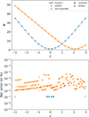 |
Fig. 1 Potential associated with a one-dimensional vertical Gaussian distribution. We considered two cases: (i) when centred around the midplane, and (ii) with a shifted Gaussian profile. |
3.2 3D test with mixed boundary conditions
A more challenging test consists of benchmarking our solver in a setup with two periodic BCs and one unbound direction. Therefore, we chose a density distribution (defined on z ∈ [−Lz/2, Lz/2]),
![Mathematical equation: $\[\rho(x, y, z)=~\cos \left(k_x x\right) ~\cos \left(k_y y\right) e^{-\frac{1}{2}(z / H)^2},\]$](/articles/aa/full_html/2026/02/aa57659-25/aa57659-25-eq27.png) (20)
(20)
whose associated potential (applicable in the same domain) is:
![Mathematical equation: $\[\Phi(x, y, z)=4 \pi G ~\cos \left(k_x x\right) ~\cos \left(k_y y\right)\left[2 a ~\cosh~ (k z)+F_{+}+F_{-}\right],\]$](/articles/aa/full_html/2026/02/aa57659-25/aa57659-25-eq28.png) (21)
(21)
with ![Mathematical equation: $\[k=\sqrt{k_{x}^{2}+k_{y}^{2}}\]$](/articles/aa/full_html/2026/02/aa57659-25/aa57659-25-eq29.png) , as well as functions
, as well as functions
![Mathematical equation: $\[\begin{aligned} F_{ \pm}(z) =\sqrt{\frac{\pi}{2}} \frac{H}{2 k} e^{\frac{k H}{2}(k H \pm 2 z / H)} \operatorname{erf}\left(\frac{k H \pm z / H}{\sqrt{2}}\right) \\ a \qquad =-\sqrt{\frac{\pi}{2}} \frac{H}{2 k} e^{\frac{(k H)^2}{2}} \operatorname{erf}\left(\frac{k H+L_z /(2 H)}{\sqrt{2}}\right)\end{aligned}\]$](/articles/aa/full_html/2026/02/aa57659-25/aa57659-25-eq30.png) (22)
(22)
As in Sect. 3.1, we also obtained this solution by solving the Poisson equation in the vacuum regions and enforcing the continuity of both the potential and its derivative at the domain boundaries. However, unlike in Sect. 3.1, we additionally imposed the condition that the potential vanishes at large distances from the midplane (see Sect. 2.3).
For this study, we set Nx = Ny = Nz = 128, as well as Lx = Ly = Lz = 6, and chose the scale height a) three times smaller than the vertical extent of the box, and b) as large as the latter – in other words H ∈ [1.0, 3.0]. In addition, we set kx = ky = 2π/Lx.
In Fig. 2, we display the gravitational potential, for x = y = 0, as a function of z in the top panel and the associated relative error in the bottom panel. As previously, we subtracted a constant from all potentials to ensure that their minima were equal to 1. For both configurations, the relative error of the VGF-HybridBC approach reached its maximum at the vertical boundaries. The upper limits on the error are about 10−6 and 10−4, for H = 1.0 and H = 3.0, respectively. Note that the error vanishes exactly in the symmetry plane (i.e. at z = 0). In comparison, the SASHA approach is slightly less accurate (by a factor of a few in terms of relative error) than the VGF-HybridBC method revisited.
For completeness, in Fig. 3 we show the colour-coded relative error in the z = 0 plane (top) and the y = 3 plane (bottom), respectively. The overall error was less than 10−5 (with the maximum reached near the vacuum boundaries), including larger regions where the error was exactly zero (i.e. below machine accuracy).
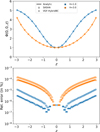 |
Fig. 2 Potential along the z direction associated with a 3D density distribution: periodic in x and y, Gaussian in the vertical direction. |
3.3 Numerical convergence
For the numerical convergence test, we conducted 1D and 3D tests as outlined in Sects. 3.1 and 3.2, varying the number of cells from 163 to 2563. Figure 4 displays the L2 norm of the relative error,
![Mathematical equation: $\[\|\epsilon\|_2=\frac{1}{N} \sqrt{\sum_{i, j, k} \epsilon_{i, j, k}^2}\]$](/articles/aa/full_html/2026/02/aa57659-25/aa57659-25-eq31.png) (23)
(23)
for both 1D (top panel) and 3D (bottom panel) cases. We begin by analysing the outcomes of the SASHA method. In the 1D test, errors exhibit third-order convergence, with the highest error observed for the shifted distribution. Conversely, in the 3D test, this method demonstrates second-order convergence. Moving on to the VGF-HybridBC method, we find that in both scenarios, errors converge at a third order. The worst-case error is approximately 10−5, with the best-case error reaching 10−7 for 163 cells. For 2563 cells, the error for all tests is consistently below 10−9 and reaches as low as 10−11 for the 3D test with H = 1.
3.4 Jeans instability
This 1D dynamical test consists of triggering gravitational instability of a uniform density distribution at equilibrium, and is particularly tailored to solving the Poisson equation with periodic BC. Therefore, we consider a 1D box with 128 cells is the x direction and consider a uniform density distribution, augmented by a small sinusoidal perturbation:
![Mathematical equation: $\[\rho(x)=\rho_0\left(1+A \cos \left(\frac{2 \pi x}{\lambda}\right)\right)\]$](/articles/aa/full_html/2026/02/aa57659-25/aa57659-25-eq32.png) (24)
(24)
with A = 0.01. This perturbation can lead to either oscillating short-wavelength perturbations or to collapsing long-wavelength modes (Hubber et al. 2006; Mandal et al. 2023), whose periods and time, respectively, are
![Mathematical equation: $\[T_{\mathrm{osc}}=\left(\frac{\pi}{G \rho_0}\right)^{1 / 2} \frac{\lambda}{\left(\lambda_J^2-\lambda^2\right)^{1 / 2}}; ~T_{\mathrm{coll}}=\left(\frac{1}{4 \pi G \rho_0}\right)^{1 / 2} \frac{\lambda}{\left(\lambda^2-\lambda_J^2\right)^{1 / 2}},\]$](/articles/aa/full_html/2026/02/aa57659-25/aa57659-25-eq33.png) (25)
(25)
where ![Mathematical equation: $\[\lambda_{J}=\sqrt{\frac{\pi c_{s}^{2}}{G \rho_{0}}}\]$](/articles/aa/full_html/2026/02/aa57659-25/aa57659-25-eq34.png) is the Jeans length. Specifically, the collapse time is the time it takes for the peak density to grow from Aρ0 to Aρ0 cosh (1). As in Mandal et al. (2023), we fix λ = 2 and vary the ratio λ/λJ, which is equivalent to changing the sound speed. This choice makes it possible to have one perturbation normal mode in the initial state for all setups.
is the Jeans length. Specifically, the collapse time is the time it takes for the peak density to grow from Aρ0 to Aρ0 cosh (1). As in Mandal et al. (2023), we fix λ = 2 and vary the ratio λ/λJ, which is equivalent to changing the sound speed. This choice makes it possible to have one perturbation normal mode in the initial state for all setups.
In Fig. 5, we depict the normalised time (i.e. with respect to the free fall time) with respect to the normalised wavelength. The star and circles correspond to the fitted numerical points in the oscillatory and collapsing regimes, respectively, while the solid lines are the theoretical estimates. We observe that the error between the theoretical prediction and the numerical estimate is smaller than 0.3% in the oscillatory regime, and about 2% in the collapsing regime, which validates this test.
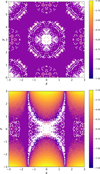 |
Fig. 3 Log-scale relative error cuts for the 3D test, employing the VGF-HybridBC method, with mixed BCs. Top: z = 0 plane. Bottom: y = 3 plane. |
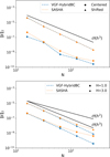 |
Fig. 4 Convergence test: 1D (top) and 3D (bottom) results. The SASHA technique achieves second-order convergence, while the VGF-HybridBC method reaches slightly better than third-order convergence. |
4 Performance estimates
We benchmarked the real-life performance of our algorithm on the Romeo cluster at the HPC Centre at the TU Dresden2. Specifically, that machine is a general-purpose NEC cluster featuring 188 nodes, each equipped with dual AMD EPYC 7702 processors (64 cores @ 2.0 GHz, multithreading enabled), 512 GB of DDR4-3200 RAM, and 200 GB of local SSD storage. We employed the exclusive option of SLURM to mitigate interference with other jobs.
For the presented weak scaling test, each MPI task handled a fixed workload of 323 cells. We emphasize that for a fixed number of cores, P3DFFT performs optimally for a processor grid configuration satisfying Py ≥ Px, where Px and Py denote the number of processors in the x and y directions, respectively. Additionally, Py should be set to the maximum number of logical cores per node, which is 128 for the ROMEO cluster. In contrast, the MHD solver achieves optimal performance with a grid decomposition that minimizes the surface-to-volume ratio. For our setup, this implies that Px should be as close as possible to Py. To reconcile these conflicting requirements, we tested multiple processor grid decompositions for a fixed number of cores, adopting the configuration with the minimal runtime as the baseline for each core count.
In Fig. 6, we present the scaling of the VGF-HybridBC method, implemented in the finite volume code nirvana-iii, from 128 to 4096 processors. For completeness, we compared the timings of our spectral solver with those of the orbital advection, mesh synchronization, and MHD solver. We found that the time spent in a) the interpolation to the nearest periodic point, and b) the spectral solver, increases with the total number of cell points, but its share in the total computation time remains almost constant and below 6%.
We emphasize that the timings of our solver are problem-independent: spectral methods do not require iterations that depend on the problem, and the number of operations is fixed for a given grid size, regardless of the density distribution. Therefore we expect to maintain the obtained performance in any kind of production runs.
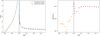 |
Fig. 5 Left: characteristic times of oscillatory and collapse modes with respect to wavelength. Right: relative error. |
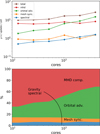 |
Fig. 6 Weak scaling study for a workload of 323 cells per MPI task and using pencil decomposition (P3DFFT). The time spent in the spectral solver is less than 6% of the whole runtime. |
5 Conclusion
We have presented two novel spectral methods for solving the Poisson equation, tailored for Cartesian shearing box simulations with vertical vacuum BCs. Our first method, SASHA, combines an analytical solution with a spectral solution via the superposition principle. Our second approach, VGF-HybridBC, leverages the free-space nature of the Green’s function, yielding an analytical and regularized expression in Fourier space (Eq. (14)). This last approach allows the gravitational potential to be evaluated in a single step as a 3D convolution in Fourier space. This enables the use of fast Fourier algorithms, achieving high performance and accuracy.
We implemented these new methods in the Finite Volume code NIRVANA-III. To optimize performance, we integrated both methods with the P3DFFT library. This allows for pencil decomposition, balancing the computational load between the hydrodynamic solver and the spectral solver. Our results demonstrate excellent accuracy, with a relative error of at least 10−5 using only 163 grid cells. The methods, SASHA and VGF-HybridBC, demonstrate second- and third-order convergence, respectively. In a standard production run using orbital advection, our spectral solver accounts for less than 6% of the total runtime, even when scaled up to 4096 processors.
Acknowledgements
This work was supported by the European Union (ERC-CoG, EPOCH-OF-TAURUS, No. 101043302). Views and opinions expressed are however those of the author(s) only and do not necessarily reflect those of the European Union or the European Research Council. Neither the European Union nor the granting authority can be held responsible for them. The authors gratefully acknowledge the computing time made available to them on the high-performance computer at the NHR Center of TU Dresden. This center is jointly supported by the Federal Ministry of Education and Research and the state governments participating in the NHR (www.nhr-verein.de/unsere-partner).
References
- Armitage, P. J., Livio, M., & Pringle, J. E. 2001, MNRAS, 324, 705 [NASA ADS] [CrossRef] [Google Scholar]
- Baehr, H., & Zhu, Z. 2021, ApJ, 909, 136 [NASA ADS] [CrossRef] [Google Scholar]
- Binney, J., & Tremaine, S. 2008, Galactic Dynamics, 2nd edn. (Princeton University Press) [Google Scholar]
- Deng, H., Mayer, L., & Latter, H. 2020, ApJ, 891, 154 [Google Scholar]
- Frigo, M., & Johnson, S. G. 2005, Proc. IEEE, 93, 216 [Google Scholar]
- Gammie, C. F. 2001, ApJ, 553, 174 [Google Scholar]
- Goldreich, P., & Lynden-Bell, D. 1965, MNRAS, 130, 125 [Google Scholar]
- Gressel, O., & Ziegler, U. 2007, Comput. Phys. Commun., 176, 652 [Google Scholar]
- Gressel, O., & Ziegler, U. 2024, Astron. Nachr., 345, e20240056 [Google Scholar]
- He, C.-C., & Ricotti, M. 2023, MNRAS, 522, 5374 [Google Scholar]
- Hockney, R. W., & Eastwood, J. W. 1981, Computer Simulation Using Particles (Taylor & Francis) [Google Scholar]
- Hubber, D. A., Goodwin, S. P., & Whitworth, A. P. 2006, A&A, 450, 881 [NASA ADS] [CrossRef] [EDP Sciences] [Google Scholar]
- James, R. A. 1977, J. Computat. Phys., 25, 71 [Google Scholar]
- Johansen, A., Youdin, A., & Klahr, H. 2009, ApJ, 697, 1269 [Google Scholar]
- Koyama, H., & Ostriker, E. C. 2009, ApJ, 693, 1316 [NASA ADS] [CrossRef] [Google Scholar]
- Kratter, K., & Lodato, G. 2016, ARA&A, 54, 271 [Google Scholar]
- Löhnert, L., & Peeters, A. G. 2023, A&A, 677, A173 [NASA ADS] [CrossRef] [EDP Sciences] [Google Scholar]
- Mandal, A., Mukherjee, D., & Mignone, A. 2023, ApJS, 268, 40 [NASA ADS] [CrossRef] [Google Scholar]
- Mayani, S., Montanaro, V., Cerfon, A., et al. 2024, arXiv e-prints [arXiv:2405.02603] [Google Scholar]
- Moon, S., Kim, W.-T., & Ostriker, E. C. 2019, ApJS, 241, 24 [Google Scholar]
- Norman, M. L., Wilson, J. R., & Barton, R. T. 1980, ApJ, 239, 968 [Google Scholar]
- Pekurovsky, D. 2012, SIAM J. Sci. Comput., 34, C192 [Google Scholar]
- Riols, A., & Latter, H. 2019, MNRAS, 482, 3989 [Google Scholar]
- Shu, F. H. 1977, ApJ, 214, 488 [Google Scholar]
- Stone, J. M., & Gardiner, T. A. 2010, ApJS, 189, 142 [NASA ADS] [CrossRef] [Google Scholar]
- Vico, F., Greengard, L., & Ferrando, M. 2016, J. Computat. Phys., 323, 191 [Google Scholar]
- Vorobyov, E. I., & Basu, S. 2006, ApJ, 650, 956 [CrossRef] [Google Scholar]
- Ziegler, U. 2005, A&A, 435, 385 [NASA ADS] [CrossRef] [EDP Sciences] [Google Scholar]
- Zier, O., & Springel, V. 2023, MNRAS, 520, 3097 [NASA ADS] [CrossRef] [Google Scholar]
- Zou, J., Kim, E., & Cerfon, A. J. 2021, arXiv e-prints [arXiv:2103.08531] [Google Scholar]
For the simple case of a constant density, it can be shown that this is the equivalent of a parabola with its vertex at the centre of mass location (cf. the argument in Sect. 2.2, above).
Appendix A Green’s function in Fourier space
In this section we detail the derivation of the Fourier transform of the Green’s function associated with the VGF-HybridBC method:
![Mathematical equation: $\[\hat{\mathcal{G}}^L(k, k_z)=\int_{-\infty}^{\infty} \mathcal{G}^L(z) e^{i k_z z} \mathrm{~d} z.\]$](/articles/aa/full_html/2026/02/aa57659-25/aa57659-25-eq35.png) (A.1)
(A.1)
Following the definition of the Green’s function in real space (Eqs. 10 and 12), two cases must be distinguished:
-
The case k = 0:
![Mathematical equation: $\[\begin{aligned}\hat{\mathcal{G}}^L\left(k=0, k_z\right) & =\int_{-L}^L \frac{|z|}{2} e^{i k_z z} \mathrm{~d} z, \\& =\int_0^L z ~\cos~ \left(k_z z\right) \mathrm{d} z,\qquad\qquad\quad. \\& =\frac{k_z L ~\sin~ \left(k_z L\right)+\cos~ \left(k_z L\right)-1}{k_z^2}\end{aligned}\]$](/articles/aa/full_html/2026/02/aa57659-25/aa57659-25-eq36.png) (A.2)
(A.2)Expanding above expression to second order in kz and taking the limit kz → 0, we find
![Mathematical equation: $\[\hat{\mathcal{G}}^L\left(k=0, k_z=0\right)=\frac{L^2}{2}.\]$](/articles/aa/full_html/2026/02/aa57659-25/aa57659-25-eq37.png) (A.3)
(A.3) The case k ≠ 0:
![Mathematical equation: $\[\begin{aligned}\hat{\mathcal{G}}^L(k=0, k_z) & =-\frac{1}{2 k} \int_{-L}^L e^{-k|z|} ~e^{i k_z z} \mathrm{~d} z, \\& =-\frac{1}{k} \int_0^L ~\cos~ \left(k_z z\right) e^{-k z} \mathrm{~d} z, \\& =-\frac{e^{-k L}\left(\frac{k_z}{k} ~\sin~ \left(k_z L\right)-\cos~ \left(k_z L\right)\right)+1}{k^2+k_z^2}.\end{aligned}\]$](/articles/aa/full_html/2026/02/aa57659-25/aa57659-25-eq38.png) (A.4)
(A.4)
All Figures
|
Fig. 1 Potential associated with a one-dimensional vertical Gaussian distribution. We considered two cases: (i) when centred around the midplane, and (ii) with a shifted Gaussian profile. |
| In the text | |
|
Fig. 2 Potential along the z direction associated with a 3D density distribution: periodic in x and y, Gaussian in the vertical direction. |
| In the text | |
|
Fig. 3 Log-scale relative error cuts for the 3D test, employing the VGF-HybridBC method, with mixed BCs. Top: z = 0 plane. Bottom: y = 3 plane. |
| In the text | |
|
Fig. 4 Convergence test: 1D (top) and 3D (bottom) results. The SASHA technique achieves second-order convergence, while the VGF-HybridBC method reaches slightly better than third-order convergence. |
| In the text | |
|
Fig. 5 Left: characteristic times of oscillatory and collapse modes with respect to wavelength. Right: relative error. |
| In the text | |
|
Fig. 6 Weak scaling study for a workload of 323 cells per MPI task and using pencil decomposition (P3DFFT). The time spent in the spectral solver is less than 6% of the whole runtime. |
| In the text | |
Current usage metrics show cumulative count of Article Views (full-text article views including HTML views, PDF and ePub downloads, according to the available data) and Abstracts Views on Vision4Press platform.
Data correspond to usage on the plateform after 2015. The current usage metrics is available 48-96 hours after online publication and is updated daily on week days.
Initial download of the metrics may take a while.