| Issue |
A&A
Volume 707, March 2026
|
|
|---|---|---|
| Article Number | A181 | |
| Number of page(s) | 7 | |
| Section | The Sun and the Heliosphere | |
| DOI | https://doi.org/10.1051/0004-6361/202553874 | |
| Published online | 05 March 2026 | |
Three-dimensional numerical experiments on granulation-generated, two-fluid waves and flows in a solar magnetic carpet
Institute of Physics, University of M. Curie-Skłodowska Pl. M. Curie-Skłodowskiej 1 20-031 Lublin, Poland
★ Corresponding author: This email address is being protected from spambots. You need JavaScript enabled to view it.
Received:
23
January
2025
Accepted:
17
December
2025
Abstract
Context. These studies were carried out in the context of solar-chromosphere heating and solar-wind generation.
Aims. We aim to explore granulation-generated, two-fluid waves and flows in the solar atmosphere permeated by a solar magnetic carpet.
Methods. Three-dimensional (3D) numerical experiments were performed with the use of the JOANNA code, to solve two-fluid equations for ions+electrons and neutrals treated as two separate interacting fluids. We assumed that the plasma is hydrogen and initially described by a hydrostatic state supplemented by the Saha equation. Two model cases were considered: (a) two-fluid equations with ionisation, recombination and radiation switched on; and (b) ideal two-fluid equations.
Results. We find that the granulation-generated perturbations in a two-fluid regime and a partially ionised solar chromosphere result in the self-consistent evolution of waves, flows, and the ionisation ratio in the chromosphere and the low corona. In particular, as a result of radiative cooling and recombination as well as jets, which inject partially ionised plasma, the number of neutrals increases in the low corona, and the Fourier spectrum of the excited waves shows some level of convergence to the observational data. Compared to previous findings, ionisation, recombination and radiation result in a larger movement upwards of the transition region, whereas in the idealised case the transition region essentially does not experience its vertical shift by the developed granulation.
Conclusions. We infer that 3D effects and the ionisation and recombination operating simultaneously with radiation play a role in evolution of the solar atmosphere, affecting, among a diversity of phenomena, granulation-excited waves, flows, jets, and ionisation levels.
Key words: Sun: activity / Sun: atmosphere / Sun: granulation
© The Authors 2026
 Open Access article, published by EDP Sciences, under the terms of the Creative Commons Attribution License (https://creativecommons.org/licenses/by/4.0), which permits unrestricted use, distribution, and reproduction in any medium, provided the original work is properly cited.
This article is published in open access under the Subscribe to Open model. This email address is being protected from spambots. You need JavaScript enabled to view it. to support open access publication.
1. Introduction
Due to its internal structure and physical properties, the solar atmosphere is divided into three main layers. The deepest layer is the photosphere, which is characterised by a temperature of about T = 5800 K. Such a low temperature results in a large fraction of neutral atoms there (Vernazza et al. 1981). In the higher layer, known as the chromosphere, the temperature rises to about 7 ⋅ 103 K, where the ion-neutral collision frequency decreases and the charged and neutral fluids begin to decouple. Hence, we have to take neutrals into account in a description of plasma dynamics in this layer. The chromosphere is caped by the solar corona, where the temperature grows to 1–3 MK, essentially leading to complete ionisation of the plasma.
The rise in temperature in the solar atmosphere is the central conundrum of heliophysics. To study processes in the atmosphere layers, one must understand their dynamics, which is highly dependent on the magnetic field. Most of the magnetic flux is present in the flux tubes with magnetic lines that fan out and magnetic carpet ingredients (Kuridze et al. 2015; Srivastava et al. 2017). The interaction of the flux tubes with the convection zone leads to a generation of transverse and longitudinal waves (Musielak et al. 2002; Fawzy 2010). Torsional waves predicted by Alfvén (1942) are particularly important since they transport their energy along the magnetic-field lines (Vasheghani Farahani et al. 2011, 2012; Murawski et al. 2015). It was shown by Kuźma & Murawski (2018) that fast, magnetoacoustic kink waves can also be guided by flux tubes. Recent observational and theoretical studies of magnetohydrodynamic (MHD) waves were performed by Nakariakov & Kolotkov (2020). However, for chromosphere heating it is essential to consider ion-neutral collisions that appear inherently in the two-fluid plasma model (Soler et al. 2015; Ballester et al. 2018; Alharbi et al. 2022).
A study of granulation-generated, two-fluid waves by Murawski et al. (2022) revealed that the energy released in ion-neutral collisions (with non-ideal and non-adiabatic effects) can partially compensate the radiative and thermal losses in the chromosphere. 2D numerical experiments on granulation-generated waves performed by Niedziela et al. (2024b) for weak and strong magnetic carpets show a correlation of the magnitude of the magnetic field, plasma flows, and heating. 3D numerical simulations of the granulation-excited two-fluid waves, plasma flows, and the associated chromosphere heating were performed by Murawski et al. (2020). However, the adopted model assumed the hydrostatic initial state, while a more realistic ionisation profile requires supplementing this state with the Saha ionisation profile (Saha 1920). The goal of this paper is to improve the models of Murawski et al. (2020) and Niedziela et al. (2024b) by taking the Saha equation into account and implementing a magnetic carpet in a 3D solar atmosphere.
The remainder of this paper is organised as follows. Section 2 describes the numerical model, Section 3 presents and discusses the corresponding results, and Section 4 contains a summary and an analysis of the obtained results.
2. Numerical model
The solar atmosphere is described by two-fluid equations for ions (protons) + electrons and neutrals (hydrogen atoms). The model was discussed in some detail in Murawski et al. (2022) and recently used by Niedziela et al. (2024b) to simulate 2D solar granulation with a magnetic carpet. To reduce the numerical cost of 3D simulations, all non-ideal (viscosity, magnetic resistivity) and non-adiabatic (thermal conduction) terms – i.e. processes that lead to energy exchange not accounted for in the adiabatic approximation – are neglected, and only ionisation, recombination and solar radiation are considered (Murawski et al. 2022). These neglected terms may significantly influence wave propagation and damping in the solar atmosphere. In particular, we should expect thermal conduction to influence wave behaviour by diffusing thermal energy and reducing the intensity of plasma heating. All fluid quantities corresponding to electric charges and neutrals have the subscript i and n, respectively. The symbols 𝜚i, n, Vi, n = [Vi, nx, Vi, ny, Vi, nz], and Ti, n denote mass densities, velocities, and temperatures, respectively. The solar gravity works in the negative y−direction.
Initially (at t = 0 s), the system is set to be in hydrostatic state, which takes the Saha equation (Saha 1920) into account (Niedziela et al. 2024a). This state is overlaid by a magnetic field given by
![Mathematical equation: $$ \begin{aligned} \mathbf B&= B_{\rm a} \left[\cos \left(\frac{x+L_{\rm B}}{\Lambda _B}\right), -\sin \left(\frac{x+L_{\rm B}}{\Lambda _B}\right), 0\right] e^{-y/\Lambda _B} \nonumber \\&\quad +\left[B_{\rm x}, B_{\rm y}, B_{\rm z}\right]\, . \end{aligned} $$](/articles/aa/full_html/2026/03/aa53874-25/aa53874-25-eq1.gif) (1)
(1)
Here, ΛB = 2LB/π, LB = 0.64 Mm, Ba = 0.2 G is the magnetic field corresponding to a magnetic carpet, and Bx = 0 G, By = −5 G, and Bz = 0 G are the magnitudes of horizontal, vertical, and transversal components of the magnetic field, respectively. We specify the 3D numerical domain along all directions as (−5.12 ≤ x ≤ 5.12) Mm × (−3 ≤ y ≤ 7.24) Mm × (−5.12 ≤ z ≤ 5.12) Mm in the fine grid zone, which is covered by 128 × 128 × 128 cells. Above the y = 7.24 Mm level, the grid is stretched in a vertical direction to y = 15 Mm and covered by only 32 cells. Such a low number of grid points was chosen to absorb the incoming wave signal. At the bottom and top boundaries, all plasma quantities are fixed to their initial values, while at the four vertical sides periodic boundaries are implemented. Initial seeding of granulation was done by a small random signal in Vi, ny, which varies along the x and z directions. This results in variations of the system along z, despite the initial magnetic and thermodynamic variables being independent of this coordinate. The following two cases were considered:
-
(a)
two-fluid equations with ionisation, recombination and solar radiation taken into account
-
(b)
ideal two-fluid equations with all non-ideal and non-adiabatic terms switched off.
3. Numerical results
In this part of the paper, we present numerical results for the granulation-generated, two-fluid waves and flows.
3.1. Evolution of ions
Figure 1 illustrates the spatial profiles of log(Ti(x, y, z, t = 5000 s)) in the (a) top and (b) bottom cases. Note the perturbations of the transition region, which was initially located at y = 2.1 Mm. As time progresses, the initial state is altered by self-generated and self-evolving solar granulation taking place in the photosphere, where turbulent flows result from convective instabilities.
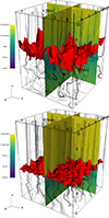 |
Fig. 1. Vertical profiles of log(Ti(x, y, z)) (colour map in the perpendicular vertical planes) and isosurfaces of Ti = 2 ⋅ 104 K (a) and Ti = 105 K (b) (red) overlaid by magnetic-field lines at t = 5000 s in the cases of (a) (top) and (b) (bottom). |
This granulation leads to the release of thermal energy and the generation of plasma jets. Note magnetic cocoons in the form of magnetic islands with zero magnetic points. Recently, such cocoons were found by Jelínek & Karlický (2024) in their numerical simulations of the solar atmosphere. The formation of the cocoons is observed in both the (a) and (b) cases, and they are present, for instance, at (x = 1, y = −1.5, z = 1) Mm in the (a) case; they are also related to the interaction of the plasma turbulence with the magnetic field. The isosurface plots correspond to T = 2 ⋅ 105 K, which show undulations of the plasma.
The numerical results are presented using horizontally and temporally averaged plasma quantities:
 (2)
(2)
 (3)
(3)
Here, t1 = 1500 s, t2 = 5000 s, x2 = z2 = −x1 = −z1 = 5.12 Mm, and f is a plasma quantity, such as a vertical component of ion velocity, Viy, and ion temperature, Ti.
Figure 2 presents horizontal slices through the lower layer of the simulation domain at t = 2000 s. The velocity field exhibits a complex distribution of upward and downward plasma motions. These structures indicate the presence of fine-scale dynamical activity and turbulence. Red regions denote upflows of hot plasma at the centres of granules, while the surrounding blue lanes represent cooler, descending plasma. The temperature distribution (bottom) reveals a similarly structured pattern, with localised regions of heating and cooling. The spatial correlation between velocity and temperature variations is characteristic for the granulation pattern and convective-energy transport. Thus, it suggests that plasma motion plays a key role in thermal-energy distribution at the bottom of the photosphere. Granulation develops after about 1500 s, when the first granules become visible. The characteristic size of granules is approximately 200 km–1 Mm.
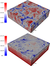 |
Fig. 2. Horizontal cut (x, z) of Viy(x, y, z) (top) and Ti(x, y, z) (bottom) at the lower layers of simulation domain at t = 2000 s in the case of (a). |
Figure 3 shows time-distance plots for ⟨Viy⟩xz (left) and ⟨Ti⟩xz (right), which denote the averaged-over horizontal coordinates x and z in the (a) (top) and (b) (bottom) cases. Note that ⟨Viy⟩xz attains both negative and positive values corresponding to down-flows and up-flows, respectively (left). However, after the initial transient phase, which lasts until t ≈ 1500 s, the atmosphere is dominated by down-flows. They are seen in the time-averaged plots (Fig. 4, left), where ⟨Viy⟩xzt < 0, in an almost entirely numerical domain, is associated with a net down-flow. It is apparent that ionisation, recombination and radiation resulted in the net rise of the transition region to about y = 3.5 Mm. This rise is larger than in the (b) case, in which the transition region remained at t = 5000 s at essentially its initial position, y = 2.1 Mm. Hence, we infer that ionisation, recombination and solar radiation results in a larger movement of the transition region.
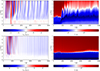 |
Fig. 3. Time-distance plots for ⟨Viy⟩xz (left) and ⟨Ti⟩xz (right) in the cases of (a) (top) and (b) (bottom). |
Note that in both cases max(⟨Viy⟩xz) is essentially the same. Additionally, for (a) there are more down-flows and lower values of ⟨Viy⟩xzt, which is particularly clear in the solar corona (Fig. 4, bottom left).
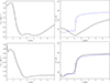 |
Fig. 4. Vertical profiles of ⟨Viy⟩xzt (left) and ⟨Ti⟩xzt (right) in the cases of (a) (top) and (b) (bottom). |
After the initial transient phase, the transition region strongly oscillates, rising to y ≈ 5 Mm (Fig. 3, top right). Note that after t = 1500 s, the offset of the transition region is about 3 Mm. This offset is the difference between the final and initial heights of the transition region.
Besides magnetic-field reshuffling, granulation is also responsible for wave generation (Fig. 1). Figure 5 displays periods obtained from the Fourier spectra for 〈Viy〉xz (Figs. 3 and 4, left). We took these spectra for 1500 s ≤ t ≤ 5000 s. The numerical results show partial agreement with the observational data obtained by Wiśniewska et al. (2016) and Kayshap et al. (2018). The simulated wave periods in the (b) case lie within the observed range (150–300 s) and exhibit a similar trend of decreasing period up to ∼1.2 Mm. However, in the (a) case, the range of obtained periods is larger than in observational data. At the heights within the 0 Mm < y < 1 Mm range, it is observed that the dominant wave period is about P = 300 s in the (a) case, while in the (b) case we find P ≈ 220 s within the 0.5 Mm < y < 3 Mm range. In the (a) case for y < −0.2 Mm and y > 1.6 Mm, the dominant wave period corresponds to P ≈ 350 s. It is well known that magnetoacoustic waves with the period P > 300 s are evanescent in the photosphere (e.g. Zaqarashvili et al. 2011), and therefore, the waves of these periods are unable to extend to higher altitudes. It means that the cut-off period (Wójcik et al. 2018) of the atmosphere is significantly altered by two-fluid effects, with ionization, recombination and radiation taken into account. This alteration should be balanced by such effects as thermal conduction, which is absent from the developed models. In the regions of low-plasma β, the dominant wave modes are essentially slow magnetoacoustic waves.
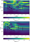 |
Fig. 5. Fourier power spectrum of wave period P for Viy versus height y in the (a) (top) and (b) (bottom) cases. The diamonds and dots represent the observational data of Wiśniewska et al. (2016) and Kayshap et al. (2018), respectively. |
3.2. Evolution of neutrals
In this part of the paper, we briefly discuss the evolution of neutrals. Figure 6 shows time-distance plots for the frictional heating term Q (first term on the RHS of Eq. 17 in Murawski et al. 2022) in the (a) (top) and (b) (bottom) cases. Both cases show the highest values of Q in the chromosphere. Frictional heating does not show as a constant band of heat but as a series of impulsive events. This pattern is directly correlated with the waves and shocks visible in Fig. 3.
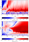 |
Fig. 6. Time-distance plots for frictional heating term Q in the (a) (top) and (b) (bottom) cases. |
The evolution of neutrals is very well illustrated in Fig. 7, which represents spatial profiles of log(𝜚n/𝜚i) at t = 5000 s. The differences between cases (a) (top) and (b) (bottom) show that taking ionisation into account results in higher log(𝜚n/𝜚i) values in the solar corona. These differences illustrate the influence of radiation and recombination on the ionisation structure.
 |
Fig. 7. Spatial profiles of log(𝜚n/𝜚i) at t = 5000 s in the case of (a) (top) and (b) (bottom). |
Figure 8 displays time-distance plots for a horizontally averaged neutral-to-ion mass density ratio, ⟨𝜚n/𝜚i⟩xz, (left) and vertical component of ion-neutral velocity drag, ⟨Viy − Vny⟩xz (right), in the (a) (top) and (b) (bottom) cases. Note that ⟨𝜚n/𝜚i⟩xz only evolves significantly in time in the (a) case. As a result of the jets, which eject chromospheric material into the solar corona, which is particularly clear in the transient phases, we see more neutrals than ions in the corona as time progresses. ⟨Viy − Vny⟩xz reaches its lowest values in the low solar corona for t < 1000 s (Fig. 8, top right), which means that at y > 2.1 Mm neutrals move upward faster than ions on average, and therefore they experience the downward-directed drag force, while ions feel the opposite reaction. We observe a similar trend in the (b) case after t > 2000 s. In the time-distance plots, there are also red patches located in the low corona for t < 1000 s and in the middle chromosphere for t > 3000 s, where ions move faster than neutrals.
 |
Fig. 8. Time-distance plots for ⟨𝜚n/𝜚i⟩xz (left) and vertical component of ion-neutral velocity drag, ⟨Viy − Vny⟩xz, (right) in the case of (a) (top) and (b) (bottom). |
4. Discussion
Although further work could explore the role of additional physical processes in greater detail, comparisons with previous studies highlight the importance of including 3D effects, ionisation, recombination, and radiation.
The inclusion of a small-scale, mixed-polarity magnetic field at the lower boundary mimics the observed magnetic carpet of the quiet Sun (Thornton & Parnell 2011). This configuration leads to reconnection events, forms dynamic current sheets, and drives upward-propagating waves. While reconnection-driven solar-wind acceleration may be insufficient in quiet-Sun regions (Cranmer & van Ballegooijen 2010), the magnetic carpet still provides a significant reservoir of magnetic energy that can drive chromospheric heating and wave excitation.
The transition region experiences oscillations, which after the initial transient phase, lasting until t = 1500 s, approach the level of y = 2.1 Mm. For comparison purposes, Murawski et al. (2020) also observed the location of the transition region at y = 2.1 Mm in their 3D simulations of granulation-generated dynamics of the solar atmosphere. However, the authors reported more up-flows after the initial transient phase, which are hardly seen in this model. Niedziela et al. (2024b) performed 2D numerical experiments for the weak magnetic carpet and reported larger jets and transition-region oscillations than for these 3D results. These may be due to the lack of thermal conduction in the (a) and (b) cases discussed in this paper.
The effect of ionisation, recombination and radiation is clearly seen on ⟨Ti⟩xzt, which is significantly different from the semi-empirical temperature profile, T(y), of Avrett & Loeser (2008) in the entire atmosphere. On the other hand, the (b) case shows better agreement with T(y) in the corona given by Avrett & Loeser (2008). Again, these effects may result from the drawbacks of the developed models, mainly from the lack of operating thermal conduction and the fact that the developed initial state, which is determined with the use of the Saha equation, may be prone to the Rayleigh–Taylor instability.
The obtained Fourier spectrum shows some level of agreement with those reported by Murawski et al. (2020), which observed P ≥ 300 s oscillations in the photosphere and upper chromosphere. However, higher up, the dominant P declined to a value lower than 300 s.
Figure 8 shows ⟨𝜚n/𝜚i⟩xz, which in the (b) case remains more stratified, and the penetration of neutrals into higher layers is suppressed. On the other hand, in the (a) case neutrals spread to higher altitudes over time, which results from upward transport of neutrals from the chromosphere, combined with the limited efficiency of ionisation in the low-density coronal plasma. Ionisation timescales are longer than wave-motion ones, so neutrals can be carried into the corona before becoming ionised (Carlsson & Stein 2002).
We observe significant vertical ion-neutral velocity drifts, ⟨Viy − Vny⟩xz, during the initial phase, but it rapidly decays afterwards, when ionisation, recombination and radiative cooling are included. These processes enhance coupling between ions and neutrals, reducing velocity drift between these two species. Parametric studies performed by Niedziela et al. (2024b) show that stronger magnetic fields lead to larger drifts and, consequently, greater heating. A comparison between Q and ⟨Viy − Vny⟩xz reveals spatial and temporal correlation. Hence, it can be seen that velocity drift affects the frictional heating term, which reaches maximum values of the order of max(Q) ≈ 3 erg cm−3 s−1 for (a) and max(Q) ≈ 2 · 10−2 erg cm−3 s−1 for (b).
5. Summary and conclusions
We performed 3D numerical simulations of a partially ionised solar atmosphere and modelled it using two-fluid equations for protons + electrons and hydrogen atoms.
The hydrostatic conditions described the initial state, supplemented by the Saha equation (Niedziela et al. 2024a), and the magnetic carpet was overlaid by a vertical magnetic field in the corona. The aim was to investigate granulation-generated waves and flows.
We summarize our results as follows. Our numerical model demonstrates that the self-generated and self-evolving solar granulation facilitates the generation of all two-fluid waves, jets, and flows. The results obtained from the Fourier spectrum exhibit dominant periods, revealing some convergence level to the observational data of Wiśniewska et al. (2016) and Kayshap et al. (2018).
The studied dynamics of the ions and neutrals show clear differences in the size of the generated jets, flows, and their oscillations. Taking into account ionisation, recombination and solar radiation effects resulted in a rise of the transition region, whereas in the idealised case, its position remained hardly altered in comparison to its initial position. It has to be admitted that the developed models do not show the whole scenario, and they require further improvements. As a result of the complexity of the solar atmosphere, these improvements would consist of formidable tasks. Therefore, such complex and challenging studies are devoted to potential future research.
Acknowledgments
The authors express gratitude to the reviewer for his/her insightful comments and ideas. KM’s work was done within the framework of the project from the Polish Science Center (NCN) Grant No. 2020/37/B/ST9/00184. Numerical simulations were run on the LUNAR cluster at the Institute of Mathematics at M. Curie-Skłodowska University in Lublin, Poland. The simulation data was visualized using Python scripts and VisIt.
References
- Alfvén, H. 1942, Nature, 150, 405 [Google Scholar]
- Alharbi, A., Ballai, I., Fedun, V., & Verth, G. 2022, MNRAS, 511, 5274 [NASA ADS] [CrossRef] [Google Scholar]
- Avrett, E. H., & Loeser, R. 2008, ApJS, 175, 229 [Google Scholar]
- Ballester, J. L., Alexeev, I., Collados, M., et al. 2018, Space Sci. Rev., 214, 58 [Google Scholar]
- Carlsson, M., & Stein, R. F. 2002, ApJ, 572, 626 [Google Scholar]
- Cranmer, S. R., & van Ballegooijen, A. A. 2010, ApJ, 720, 824 [NASA ADS] [CrossRef] [Google Scholar]
- Fawzy, D. E. 2010, New Astron., 15, 717 [Google Scholar]
- Jelínek, P., & Karlický, M. 2024, A&A, 692, A116 [NASA ADS] [CrossRef] [EDP Sciences] [Google Scholar]
- Kayshap, P., Murawski, K., Srivastava, A. K., Musielak, Z. E., & Dwivedi, B. N. 2018, MNRAS, 479, 5512 [Google Scholar]
- Kuridze, D., Henriques, V., Mathioudakis, M., et al. 2015, ApJ, 802, 26 [Google Scholar]
- Kuźma, B., & Murawski, K. 2018, ApJ, 866, 50 [CrossRef] [Google Scholar]
- Murawski, K., Solov’ev, A., Musielak, Z. E., Srivastava, A. K., & Kraśkiewicz, J. 2015, A&A, 577, A126 [NASA ADS] [CrossRef] [EDP Sciences] [Google Scholar]
- Murawski, K., Musielak, Z. E., & Wójcik, D. 2020, ApJ, 896, L1 [NASA ADS] [CrossRef] [Google Scholar]
- Murawski, K., Musielak, Z. E., Poedts, S., Srivastava, A. K., & Kadowaki, L. 2022, Ap&SS, 367, 111 [NASA ADS] [CrossRef] [Google Scholar]
- Musielak, Z. E., Rosner, R., & Ulmschneider, P. 2002, ApJ, 573, 418 [Google Scholar]
- Nakariakov, V. M., & Kolotkov, D. Y. 2020, ARA&A, 58, 441 [Google Scholar]
- Niedziela, R., Murawski, K., & Poedts, S. 2024a, A&A, 691, A254 [NASA ADS] [CrossRef] [EDP Sciences] [Google Scholar]
- Niedziela, R., Murawski, K., & Srivastava, A. K. 2024b, MNRAS, 534, 2998 [Google Scholar]
- Saha, M. N. 1920, Nature, 105, 232 [CrossRef] [Google Scholar]
- Soler, R., Ballester, J. L., & Zaqarashvili, T. V. 2015, A&A, 573, A79 [NASA ADS] [CrossRef] [EDP Sciences] [Google Scholar]
- Srivastava, A. K., Shetye, J., Murawski, K., et al. 2017, Sci. Rep., 7, 43147 [Google Scholar]
- Thornton, L. M., & Parnell, C. E. 2011, Sol. Phys., 269, 13 [Google Scholar]
- Vasheghani Farahani, S., Nakariakov, V. M., van Doorsselaere, T., & Verwichte, E. 2011, A&A, 526, A80 [NASA ADS] [CrossRef] [EDP Sciences] [Google Scholar]
- Vasheghani Farahani, S., Nakariakov, V. M., Verwichte, E., & Van Doorsselaere, T. 2012, A&A, 544, A127 [NASA ADS] [CrossRef] [EDP Sciences] [Google Scholar]
- Vernazza, J. E., Avrett, E. H., & Loeser, R. 1981, ApJS, 45, 635 [Google Scholar]
- Wiśniewska, A., Musielak, Z. E., Staiger, J., & Roth, M. 2016, ApJ, 819, L23 [Google Scholar]
- Wójcik, D., Murawski, K., & Musielak, Z. E. 2018, MNRAS, 481, 262 [CrossRef] [Google Scholar]
- Zaqarashvili, T. V., Murawski, K., Khodachenko, M. L., & Lee, D. 2011, A&A, 529, A85 [NASA ADS] [CrossRef] [EDP Sciences] [Google Scholar]
All Figures
|
Fig. 1. Vertical profiles of log(Ti(x, y, z)) (colour map in the perpendicular vertical planes) and isosurfaces of Ti = 2 ⋅ 104 K (a) and Ti = 105 K (b) (red) overlaid by magnetic-field lines at t = 5000 s in the cases of (a) (top) and (b) (bottom). |
| In the text | |
|
Fig. 2. Horizontal cut (x, z) of Viy(x, y, z) (top) and Ti(x, y, z) (bottom) at the lower layers of simulation domain at t = 2000 s in the case of (a). |
| In the text | |
|
Fig. 3. Time-distance plots for ⟨Viy⟩xz (left) and ⟨Ti⟩xz (right) in the cases of (a) (top) and (b) (bottom). |
| In the text | |
|
Fig. 4. Vertical profiles of ⟨Viy⟩xzt (left) and ⟨Ti⟩xzt (right) in the cases of (a) (top) and (b) (bottom). |
| In the text | |
|
Fig. 5. Fourier power spectrum of wave period P for Viy versus height y in the (a) (top) and (b) (bottom) cases. The diamonds and dots represent the observational data of Wiśniewska et al. (2016) and Kayshap et al. (2018), respectively. |
| In the text | |
|
Fig. 6. Time-distance plots for frictional heating term Q in the (a) (top) and (b) (bottom) cases. |
| In the text | |
|
Fig. 7. Spatial profiles of log(𝜚n/𝜚i) at t = 5000 s in the case of (a) (top) and (b) (bottom). |
| In the text | |
|
Fig. 8. Time-distance plots for ⟨𝜚n/𝜚i⟩xz (left) and vertical component of ion-neutral velocity drag, ⟨Viy − Vny⟩xz, (right) in the case of (a) (top) and (b) (bottom). |
| In the text | |
Current usage metrics show cumulative count of Article Views (full-text article views including HTML views, PDF and ePub downloads, according to the available data) and Abstracts Views on Vision4Press platform.
Data correspond to usage on the plateform after 2015. The current usage metrics is available 48-96 hours after online publication and is updated daily on week days.
Initial download of the metrics may take a while.