| Issue |
A&A
Volume 707, March 2026
|
|
|---|---|---|
| Article Number | A133 | |
| Number of page(s) | 19 | |
| Section | Stellar structure and evolution | |
| DOI | https://doi.org/10.1051/0004-6361/202554413 | |
| Published online | 03 March 2026 | |
The direct effect of a toroidal magnetic field on stellar oscillations
A revised expression for the general matrix element
Thüringer Landessternwarte Sternwarte 5 D-07778 Tautenburg, Germany
★ Corresponding author: This email address is being protected from spambots. You need JavaScript enabled to view it.
Received:
7
March
2025
Accepted:
28
December
2025
Abstract
Context. Magnetic fields affect stellar oscillations through eigenmode mixing. If the contribution of a magnetic field to the stellar oscillation frequency is weak, this mode coupling can be determined using perturbation theory. The general matrix element between two modes quantifies their coupling strength.
Aims. This study revises the calculation of the direct effect of a subsurface toroidal magnetic field on solar-like stellar oscillations and provides corrected expressions for the general matrix element and the corresponding angular kernels.
Methods. We perturbed a non-magnetic, non-rotating equilibrium stellar model using a superposition of toroidal magnetic fields. Applying quasi-degenerate perturbation theory and generalised spherical harmonics, we derived the general matrix element and computed the shifts and splitting of the multiplet frequencies. We identified selection rules for mode coupling by analysing the symmetries of the angular kernels.
Results. Previous studies underestimated the direct effect of a toroidal magnetic field by neglecting non-zero contributions in integrals over products of scalar generalised spherical harmonics. We have developed an analytical method to calculate these integrals. For a strong toroidal field located at the base of the solar convection zone, the frequency shift due to the direct effect can reach 14 nHz, which is twice as large as previously reported. Modes couple through the toroidal field only if their azimuthal orders are equal and the sum of the harmonic degrees of the modes and the magnetic field components is even. The toroidal field only partially lifts the degeneracy of multiplet frequencies, leaving modes with the same absolute azimuthal order m within a multiplet degenerate.
Conclusions. We confirm that deep toroidal magnetic fields are not responsible for the observed frequency shifts between the maximum and minimum of the solar cycle. However, although their detection is strongly impeded by the much stronger effects of near-surface fields, their existence cannot be ruled out.
Key words: Sun: helioseismology / Sun: magnetic fields / Sun: oscillations / stars: magnetic field / stars: oscillations
© The Authors 2026
 Open Access article, published by EDP Sciences, under the terms of the Creative Commons Attribution License (https://creativecommons.org/licenses/by/4.0), which permits unrestricted use, distribution, and reproduction in any medium, provided the original work is properly cited.
This article is published in open access under the Subscribe to Open model. This email address is being protected from spambots. You need JavaScript enabled to view it. to support open access publication.
1. Introduction
The magnetic field distribution in the deep interior of the Sun and the exact location of the solar dynamo remain active research topics (Charbonneau 2020; Fan 2021). These related features are driven by turbulent convective flows and large-scale dynamo mechanisms (Leighton et al. 1962; Weiss et al. 1996; Ossendrijver 2003; Miesch 2005; Fan 2009). The first significant changes in solar p-mode frequencies with the solar cycle were reported by Woodard & Noyes (1988).
Broomhall (2017) isolated the effect of the magnetic field on acoustic modes and showed that the frequencies of the solar p-modes vary in phase with the solar cycle by comparing observations between a maximum and a minimum of a solar cycle. Relatively few studies have attempted to use helioseismology to determine the internal magnetic field responsible for this frequency shift, although local magnetic features such as sunspots and near-surface flows are known to induce significant perturbations (Cally 2000; Schunker & Cally 2006; Gizon et al. 2009; Khomenko & Collados 2015; Rabello-Soares et al. 2018; Braun 2019).
General formalisms for computing multiplet frequency splittings were developed primarily to account for rotation and large-scale flow perturbations (Ritzwoller & Lavely 1991; Lavely & Ritzwoller 1992; Sekii et al. 1990; Sekii 1991; Schou et al. 1994; Hanasoge et al. 2017). Complementary local helioseismic techniques, such as ring-diagram analysis (Hill 1988; Basu et al. 1999) and time-distance helioseismology (Duvall et al. 1993; Giles 2000; Zhao & Kosovichev 2004; Hanasoge et al. 2012), have been used to infer subsurface flows and asphericities, providing independent constraints on the solar interior.
Early theoretical work on the impact of global magnetic fields on solar oscillations addressed the forward problem of frequency splitting due to rotation and axisymmetric internal magnetic fields (Gough & Thompson 1990; Dziembowski & Goode 1991). This approach was refined by Antia et al. (2000) to study magnetic fields in the convection zone. They set an upper limit of 300 kG for a toroidal magnetic field at the base of the convection zone. Baldner et al. (2009) extended this work to include a poloidal magnetic field component and compared the calculated splitting coefficients with observations over a solar cycle. They found that a combination of a poloidal and two shallow near-surface toroidal fields best reproduced the data.
Dziembowski & Goode (2004) further connected solar-cycle frequency shifts to near-surface turbulent velocity and small-scale magnetic fields, while also placing helioseismic limits on a buried toroidal field at the base of the convection zone. Antia et al. (2013) then used helioseismic measurements of angular-velocity variations to constrain the strength of internal magnetic fields. Hanasoge (2017) derived Lorentz-stress sensitivity kernels for general magnetic fields, and Das et al. (2020) further developed these results. Their framework, formulated within quasi-degenerate perturbation theory but reducible to the degenerate case for isolated multiplets, demonstrates the forward problem for both deep-toroidal and surface-dipolar magnetic configurations. These studies show that frequency shifts are particularly sensitive to near-surface perturbations and provide a formal basis for helioseismic constraints on internal magnetic fields.
Building on these helioseismic approaches, magnetoasteroseismology has explored how internal magnetic fields affect stellar oscillations beyond the Sun, particularly in red giants. In such stars a ‘fossil’ field can persist as a remnant of earlier dynamo processes (Braithwaite & Spruit 2004; Duez & Mathis 2010; Stello et al. 2016). Mathis & de Brye (2011) developed a formalism for magneto-gravito-inertial waves in magnetic, rotating stellar radiation zones, while Prat et al. (2019) applied similar ideas to compute gravity-mode frequency shifts in rapidly rotating stars. Several studies have applied these ideas to red giants, demonstrating that strong internal fields can alter mixed-mode frequencies (Bugnet et al. 2021), reduce asymptotic period spacings (Loi 2020), and depress dipole stellar oscillation modes (Fuller et al. 2015). More recent work has quantified core magnetic fields in red giants and explored the detectability of complex internal field topologies using mixed-mode asymmetries (Li et al. 2023; Das et al. 2024; Bhattacharya et al. 2024). Collectively, these works, which mostly focus on gravity modes and low-degree mixed modes (l = 1, 2), show that internal magnetic fields leave measurable signatures in stellar oscillations. This motivates extending helioseismic formalisms to asteroseismic contexts and complements our focus on p-mode perturbations.
In this context, Kiefer et al. (2017) and Kiefer & Roth (2018) provide a complementary theoretical approach and numerical results for the direct effect of a toroidal magnetic field on stellar oscillation frequencies, using quasi-degenerate perturbation theory (Lavely & Ritzwoller 1992) and properties of generalised spherical harmonics (GSHs, Dahlen & Tromp 1998). The direct effect is related to the inclusion of the Lorentz force in the wave equation, neglecting the indirect effect of the magnetic field on the stellar structure. We show that refining the assumptions used for calculating integrals over products of scalar GSHs reveals previously overlooked non-zero contributions, which can significantly affect the estimated frequency shift induced by the toroidal magnetic field.
While the approach of Das et al. (2020) applies to arbitrary fields, our work focuses on the fully analytical solution for a deep-seated toroidal field, providing explicit expressions and angular kernels that are particularly relevant to solar p-modes. In this paper, we refine the solution for the direct effect of a toroidal magnetic field on solar-like oscillations by presenting a thorough analytical method to compute integrals of scalar GSH products. We provide a corrected general matrix element and the corresponding angular kernels. Since a strong, large-scale toroidal magnetic field generated by a dynamo at the base of the convection zone is believed to produce active regions on the solar surface (Fan 2009; Charbonneau 2020), we recompute the shifts and splittings of multiplet frequencies induced by a strong, purely toroidal magnetic field at the base of the solar convection zone.
The structure of this paper is as follows. Section 2 describes the equilibrium stellar model perturbed by a magnetic field. Section 3 outlines the methods of quasi-degenerate perturbation theory. Section 4 presents the general matrix element for the direct effect of a toroidal magnetic field, the complete analytical solution for integrals over products of scalar GSHs, and the selection rules for mode coupling. Section 5 presents the shifts and splitting of unperturbed multiplet frequencies caused by a strong toroidal magnetic field at the base of the solar convection zone, which are discussed in Section 6.
2. Equilibrium model
In this section, we first introduce the eigenvalue problem for the oscillations of a non-magnetic, non-rotating star (Section 2.1). Following the approach of Kiefer et al. (2017), which is based on Lavely & Ritzwoller (1992), we then consider the magnetic field as a small perturbation to the oscillation equation (Section 2.2).
2.1. Non-magnetic, non-rotating equilibrium
The equation of motion for a gas cell in a non-rotating, non-magnetic star is given by Euler’s equation for an inviscid flow:
 (1)
(1)
where v is the local momentary velocity, p is the pressure, ρ is the density, and g is the gravitational acceleration. These reference stars are static and spherically symmetric. We present a brief derivation of the eigenvalue equation of adiabatic oscillations, whose solutions are the corresponding eigenfrequencies and eigenfunctions.
We introduced oscillations as small perturbations around the equilibrium state of the star, with equilibrium quantities labelled using the subscript 0. We assumed that all perturbations were sufficiently small to justify a linear approximation. We expressed the perturbations in the Eulerian form, denoted by a prime and defined for a quantity φ as
 (2)
(2)
The displacement of a fluid element is given by
 (3)
(3)
and its velocity can be written as
 (4)
(4)
By applying the linearisation given in Equation (2) to the equilibrium model’s quantities in the equation of motion (1) and using the velocity expression from Equation (4), we obtained
 (5)
(5)
The gravitational acceleration, g, can be replaced with the gravitational potential, Φ, defined as g = −∇Φ, where Φ satisfies Poisson’s equation ∇2Φ = 4πGρ. Considering the spherical symmetry and time-independence of the equilibrium model, we adopted the following separation ansatz for the perturbation of a quantity φ:
 (6)
(6)
where θ represents the co-latitude, ϕ denotes the longitude, Ylm(θ, ϕ) is a spherical harmonic characterised by its harmonic degree l and azimuthal order m, and ω is the angular frequency. We focused on a single eigenmode, characterised by its harmonic degree l, azimuthal order m, and eigenfrequency ωnlm. Throughout the paper, the corresponding indices on perturbation quantities φ′ and ω are omitted for notational simplicity, unless needed for clarity. This separation removes the time dependence, allowing the linearised equation of motion to be expressed as an eigenvalue problem with eigenvalue ω2 and a linear operator ℱ0:
 (7)
(7)
where, in the non-magnetic case, we applied the equation of hydrostatic equilibrium ∇p0 = ρ0g0. This form is convenient, as it generalises naturally to the equilibrium operator  in the presence of a magnetic field. This eigenvalue equation, combined with the appropriate boundary conditions, yields solutions only for specific discrete eigenvalues ω2. For each (l, m), this provides a set of eigenfrequencies ωnlm, characterised by their radial order n, which indicates the number of radial nodes (excluding a possible node at the centre) in the corresponding radial eigenfunction
  , as defined in Equation (11). At the surface, we impose zero-boundary conditions, assuming that both the pressure and the density vanish at r = R. Although a non-adiabatic atmosphere is generally necessary for completeness, it is excluded from this study for simplicity. The boundary conditions also eliminate singularities at the centre and surface, ensuring regularity. A detailed description of these boundary conditions can be found in Unno et al. (1989).
For a spherically symmetric star, the orientation of the coordinate system, which is tied to the azimuthal order m, has no physical meaning. Therefore, the eigenvalue ωnlm2 is (2l + 1)-fold degenerate with respect to m. The degenerate eigenfrequencies ωnl obtained from the boundary value problem are referred to as multiplet frequencies. To solve the boundary eigenvalue problem and determine the eigenfrequencies and eigenfunctions, we first constructed a standard stellar model using the stellar evolution code Modules for Experiments in Stellar Astrophysics (MESA; Paxton et al. 2011, 2013, 2015, 2018, 2019; Jermyn et al. 2023). Using a MESA stellar evolution model as input, we used the pulsation code GYRE (Townsend & Teitler 2013; Townsend et al. 2018) to compute the eigenfrequencies and eigenfunctions for the adiabatic oscillation modes of the model. Instead of adopting Model S (Christensen-Dalsgaard et al. 1996), we constructed a standard solar model using MESA to illustrate that our method is applicable to general stellar models beyond the solar case. The root-mean-square of the relative difference in the sound speed between our MESA solar model and Model S is only 0.2%. The remaining discrepancies are primarily due to the omission of the atmospheric layers and a simplified treatment of material mixing. For a solar model, we computed modes up to 5200 μHz with harmonic degrees reaching l = 250.
In the following, we omit the tilde to distinguish between φ′(r, θ, ϕ, t) and  , as well as the subscript 0 for equilibrium quantities, for readability, unless needed for clarity. The displacement vector ξ, of which our eigenfunctions are composed, can be explicitly derived from Equation (7) using the separation of variables (6) and the gradient in spherical coordinates (A.4):
 (8)
(8)
![Mathematical equation: $$ \begin{aligned} =&\ \Biggl \{\frac{1}{\omega ^2}\bigg (\frac{1}{\rho }\frac{\partial p^{\prime }}{\partial r}+\frac{\partial \Phi ^{\prime }}{\partial r}+\frac{\rho ^{\prime }}{\rho }g\bigg )Y_l^m\hat{\mathbf{e }}_r \nonumber \\&+\frac{1}{r\omega ^2}\bigg (\frac{p^{\prime }}{\rho }+\Phi ^{\prime }\bigg )\bigg [\frac{\partial Y_l^m}{\partial \theta }\hat{\mathbf{e }}_\theta +\frac{1}{\sin \theta }\frac{\partial Y_l^m}{{\partial \phi }}\hat{\mathbf{e }}_\phi \bigg ]\Biggr \}\text{ e}^{-i\omega t} \end{aligned} $$](/articles/aa/full_html/2026/03/aa54413-25/aa54413-25-eq12.gif) (9)
(9)
![Mathematical equation: $$ \begin{aligned} =&\ \Biggl \{\tilde{\xi }_rY_l^m\hat{\mathbf{e }}_r+\tilde{\xi }_h\bigg [\frac{{\partial Y_l^m}}{{\partial \theta }}\hat{\mathbf{e }}_\theta +\frac{1}{\sin \theta }\frac{{\partial Y_l^m}}{{\partial \phi }}\hat{\mathbf{e }}_\phi \bigg ]\Biggr \}\text{ e}^{-i\omega t} \ . \end{aligned} $$](/articles/aa/full_html/2026/03/aa54413-25/aa54413-25-eq13.gif) (10)
(10)
Here, we decompose the displacement vector into its radial and horizontal components, where  and
and  are defined as
 (11)
(11)
 (12)
(12)
2.2. Equilibrium model with magnetic field
The equation of motion (1) can be extended to include a magnetic field by adding the Lorentz force per mass (cgs units):
 (13)
(13)
where B is the magnetic field. We continue to assume a time-independent equilibrium model and neglect large-scale velocity fields, so that
To avoid confusion with the non-magnetic, non-rotating equilibrium quantities φ0, we denote the equilibrium quantities in the presence of a magnetic field by  . Under equilibrium conditions, Equation (13) simplifies to
 (14)
(14)
We introduced stellar oscillations once more by linearising all quantities φ around the equilibrium model in the presence of a magnetic field,
 (15)
(15)
By applying linearisation to Equation (13), retaining only linear-order perturbations, separating the time dependencies as in Equation (6), and incorporating Equation (14), we obtained
 (16)
(16)
The operator  is defined analogously to ℱ0 given in Equation (7), but with equilibrium quantities
  . The operator ℱB represents the direct effect of the magnetic field and is given by
![Mathematical equation: $$ \begin{aligned} {\mathcal{F} }_B(\boldsymbol{\xi }):=&-\frac{1}{4 \pi \tilde{\rho }_0}\Bigg [\bigg \{\frac{(\boldsymbol{\xi } \cdot \nabla ) \tilde{\rho }_0}{\tilde{\rho }_0} +{\nabla \cdot \boldsymbol{\xi }}\bigg \}\big (\nabla \times \tilde{\mathbf{B }}_0\big ) \times \tilde{\mathbf{B }}_0 \nonumber \\&+\big (\nabla \times \tilde{\mathbf{B }}_0\big ) \times \mathbf{B }^{\prime }+\big (\nabla \times \mathbf{B }^{\prime }\big ) \times \tilde{\mathbf{B }}_0\Bigg ] \ , \end{aligned} $$](/articles/aa/full_html/2026/03/aa54413-25/aa54413-25-eq26.gif) (17)
(17)
where the Eulerian perturbation of the magnetic field B′ is expressed using ideal magnetohydrodynamics as
 (18)
(18)
This result is consistent with Equation (19.13) in Unno et al. (1989) and Equation (2.5) in Gough & Thompson (1990). However, our result differs from Equation (24) in Kiefer et al. (2017). Kiefer et al. (2017) appears to have cancelled the density  in the first term within the curly brackets of Equation (17). This approach is incorrect because the gradient operator in the numerator still acts on the density. Eliminating the density neglects the effect of the gradient on
  , which is crucial for the correct formulation of the operator. Consequently, the analytical expressions for the operator ℱB and the general matrix element defined in Section 4 differ from those of Kiefer et al. (2017).
Equations (14) and (16) show that the magnetic field affects both the equilibrium structure and the oscillations. We considered both effects as small perturbations. To account for the change in the equilibrium structure we expanded the equilibrium quantities in the presence of a magnetic field,  , to first order around the non-magnetic, non-rotating equilibrium model given by the operator ℱ0, as follows:
 (19)
(19)
This gives
 (20)
(20)
where ℱ1 contains all linear-order perturbations to the stellar structure due to the magnetic field and is referred to as the indirect effect. The direct contribution of the magnetic field perturbation is given by ℱB, which couples the modes and thus modifies the oscillation frequencies and eigenfunctions. Although ℱB includes equilibrium structure quantities in the presence of the magnetic field, we retained only the leading-order term, since ℱB is also considered a small perturbation to the oscillation equations. Finally, we obtained the total adiabatic oscillation eigenvalue equation
 (21)
(21)
The direct and indirect effects can be separated due to the additivity of the contributions, as shown in Equation (21). Kiefer & Roth (2018) provide a calculation of the indirect effect due to a magnetic field. In this work, we focus on the direct effect of the magnetic field ℱB. We therefore neglected the indirect effect ℱ1 in Equation (21) and assumed that the equilibrium state is described by the non-magnetic, non-rotating model given by
 (22)
(22)
where k = (n, l, m).
3. Quasi-degenerate perturbation theory
The eigenfrequencies of the equilibrium model form a dense spectrum, resulting in small frequency differences between the modes relative to the oscillation frequency. Therefore, we can apply the perturbation theory of quasi-degenerate states (Lavely & Ritzwoller 1992; Roth 2002; Kiefer et al. 2017). The eigenspace K consists of eigenfunctions with nearly identical eigenfrequencies. The eigenspace K includes an eigenfunction ξ0, k only if its degenerate eigenfrequency ω0, k2 = ω0, nl2 satisfies
 (23)
(23)
where ωref2 is a reference frequency set equal to the degenerate frequency ω0, j2 of the multiplet that we want to perturb. The frequency range of the coupling modes within the eigenspace K is determined by Δω2 and provides a measure of the accuracy of the perturbed quantities.
We assumed that the change in the oscillation equation due to the direct effect of the magnetic field was a small perturbation. We therefore expanded the eigenfunctions and eigenfrequencies of a mode j to first-order as
 (24)
(24)
 (25)
(25)
 (26)
(26)
The subscripts 0 and 1 in the expansion terms refer to the zeroth- and first-order perturbations, respectively. Here, ω1, j2 represents the first-order perturbation of the squared eigenfrequency of mode j. We further expanded the zeroth- and first-order eigenfunction perturbations in terms of the unperturbed eigenfunctions according to the quasi-degenerate perturbation theory as follows:
 (27)
(27)
 (28)
(28)
where K⊥ is the orthogonal complement of K in the set of all unperturbed eigenfunctions. The expansion coefficients ajk and bjk are complex constants. We inserted the expansions (24)–(28) into the not-exactly solvable oscillation eigenvalue problem (21), discarding second- or higher-order perturbations and neglecting the indirect effect. We then computed the inner product with ρ0ξ0, k′* and the resulting expression is integrated over the volume of the star. This yields
 (29)
(29)
The unperturbed eigenfunctions satisfy the orthogonality relation (Unno et al. 1989; Lavely & Ritzwoller 1992)
 (30)
(30)
where we used the following abbreviations:
 (31)
(31)
 (32)
(32)
Using this orthogonality, together with Equation (22), and incorporating certain factors into the expansion coefficients, we derive
 (33)
(33)
where Zk′k is a component of the so-called supermatrix Z, defined for (k, k′) ∈ K as
 (34)
(34)
The last term in Equation (33) is non-zero only when k = k′∈K⊥, which decouples it from the remaining terms for k ∈ K. This yields a decoupled eigenvalue equation,
 (35)
(35)
which can also be expressed as
 (36)
(36)
where Λ is a diagonal matrix and A is the eigenvector matrix. The entries of Λ are the squared eigenfrequency perturbations, Λkj = ω1, j2δkj for j ∈ K. Each column of A corresponds to an eigenvector aj that contains the expansion coefficients such that Akj = ajk. Numerical methods can solve the eigenvalue Equation (36) for a given supermatrix Z. We define the general matrix element based on Equation (34) as
 (37)
(37)
This element represents the (m′,m) component of the general matrix Hn′n, l′l, where |m′| ≤ l′ and |m|≤l. Therefore, the component Zk′k of the supermatrix Z can also be written as
 (38)
(38)
Solving the eigenvalue Equation (36) numerically yields the squared frequency perturbations ω1, j2 and the eigenvectors aj. We used these quantities to determine the zeroth-order perturbation of the eigenfunctions  from Equation (27). We matched the frequency shift ω1, j2 with the corresponding quantum numbers (n, l, m) of the unperturbed mode by extracting the maximum component aj, kmax of the eigenvector aj. Since the perturbations are small, we assumed that the main contribution to the perturbed eigenfunction
  originates from the unperturbed eigenfunction with the same quantum numbers. Thus, the degenerate eigenfrequency ω0, x2 corresponding to the mode ξ0, kmax is subject to the frequency shift ω1, j2. The perturbed squared eigenfrequencies are then given by
 (39)
(39)
The frequency shift δωj to a mode j is defined as (Lavely & Ritzwoller 1992):
 (40)
(40)
Substituting this into Equation (39) and assuming a small perturbation while neglecting higher-order terms yields the following approximation for the frequency shift:
 (41)
(41)
4. General matrix element for a toroidal magnetic field
We derived the general matrix element corresponding to a perturbation induced by a toroidal magnetic field following the approach outlined by Kiefer et al. (2017). Our analytical results differ from those presented by Kiefer et al. (2017) because we derived a different perturbation operator (Equation (17)). We obtained the general matrix element for a magnetic field by combining Equations (17) and (37):
![Mathematical equation: $$ \begin{aligned} H_{k\prime k}=&-\frac{1}{4\pi }\int _{V}\boldsymbol{\xi }_{0,k\prime }^*\Bigg [\bigg \{\frac{( \boldsymbol{\xi }_{0,k}\cdot \nabla ) \rho _0}{\rho _0}+\nabla \cdot \boldsymbol{\xi }_{0,k}\bigg \}\big (\nabla \times \mathbf B _0\big ) \times \mathbf B _0\nonumber \\&+\big (\nabla \times \mathbf B _0\big ) \times \mathbf B ^{\prime }+\big (\nabla \times \mathbf B ^{\prime }\big ) \times \mathbf B _0\Bigg ]\text{ d}V \ . \end{aligned} $$](/articles/aa/full_html/2026/03/aa54413-25/aa54413-25-eq56.gif) (42)
(42)
Here, we omit the tilde denoting the equilibrium model under the influence of the magnetic field to focus on the direct effect and avoid confusion with the later use of the tilde notation. We modelled the magnetic field as a superposition of purely toroidal fields without longitudinal dependence. In practice, we achieved this by setting m = 0 in the generalised spherical harmonics (GSHs) of the magnetic field. Appendix D introduces the scalar GSHs. Thus, the toroidal magnetic field is expressed as
 (43)
(43)
where
 (44)
(44)
The radial profile of the toroidal field components with degree s is denoted by as(r), while the angular profile is given by the co-latitudinal derivative of the scalar GSH  . The sum over the harmonic degrees s includes only even integers to ensure the observed opposite polarities in the northern and southern hemispheres (Hathaway 2015). By inserting the toroidal magnetic field into Equation (42), applying the distributivity of vector and dot products, using the sum rule for integrals, and replacing the Eulerian perturbation of the magnetic field with Equation (18), we obtained the following:
![Mathematical equation: $$ \begin{aligned} H_{k\prime k} =&-\frac{1}{4\pi }\sum _{s,s\prime }\int _{V}{\boldsymbol{\xi }}_{0,k\prime }^*\Bigg [\bigg \{\frac{( {\boldsymbol{\xi }}_{0,k}\cdot \nabla ) \rho _0}{\rho _0}+\nabla \cdot {\boldsymbol{\xi }}_{0,k}\bigg \}\big (\nabla \times \mathbf{B }_s\big ) \times \mathbf{B }_{s\prime } \nonumber \\&+\big (\nabla \times \mathbf{B }_s\big ) \times \Big \{ \nabla \times \big ({\boldsymbol{\xi }}_{0,k} \times \mathbf{B }_{s\prime }\big )\Big \} \nonumber \\&+\bigg (\nabla \times \Big \{ \nabla \times \big ({\boldsymbol{\xi }}_{0,k} \times \mathbf{B }_s\big )\Big \}\bigg ) \times \mathbf{B }_{s\prime }\Bigg ]\text{ d}V \ , \end{aligned} $$](/articles/aa/full_html/2026/03/aa54413-25/aa54413-25-eq60.gif) (45)
(45)
where s and s′ span the same index range.
We now focus on a single summand with fixed values of s and s′ and omit the indices s and s′ using the following notations:
 (46)
(46)
 (47)
(47)
![Mathematical equation: $$ \begin{aligned} \boldsymbol{\xi }_{0,k}&=\xi _r(r)Y_{l}^{0,m}\hat{\mathbf{e }}_r+\xi _h(r)\bigg [\frac{\partial }{\partial {\theta }}Y_{l}^{0,m}\hat{\mathbf{e }}_\theta +\frac{1}{\sin \theta }\frac{\partial }{\partial {\phi }}Y_{l}^{0,m}\hat{\mathbf{e }}_\phi \bigg ] \ , \end{aligned} $$](/articles/aa/full_html/2026/03/aa54413-25/aa54413-25-eq63.gif) (48)
(48)
![Mathematical equation: $$ \begin{aligned} \boldsymbol{\xi }_{0,k\prime }^*&=\tilde{\xi }_r(r)Y_{l\prime }^{0,m\prime *}\hat{\mathbf{e }}_r+\tilde{\xi }_h(r)\bigg [\frac{\partial }{\partial {\theta }}Y_{l\prime }^{0,m\prime *}\hat{\mathbf{e }}_\theta +\frac{1}{\sin \theta }\frac{\partial }{\partial {\phi }}Y_{l\prime }^{0,m\prime *}\hat{\mathbf{e }}_\phi \bigg ] \ . \end{aligned} $$](/articles/aa/full_html/2026/03/aa54413-25/aa54413-25-eq64.gif) (49)
(49)
We chose ξr and ξh to be real-valued (Aerts et al. 2010). A straightforward but lengthy calculation provides an explicit expression for the operator of the direct effect of a toroidal magnetic field perturbation ℱB(ξ0, k), for fixed values of s and s′. Appendix B presents the operator for the direct effect of the toroidal magnetic field and the necessary computations to obtain the corresponding general matrix element. The explicit expression of the general matrix element for a fixed s and s′ is given by
![Mathematical equation: $$ \begin{aligned} H_{k\prime k}=&\int _{V}\boldsymbol{\xi }_{0,k\prime }^*{\mathcal{F} }_B(\boldsymbol{\xi }_{0,k})\rho _0\text{ d}V \nonumber \\ =&\frac{1}{4\pi }\int _{V}\Biggl [\bigg (\frac{a\tilde{a}\xi _r\tilde{\xi }_r}{r}\frac{\partial {\ln \rho _0}}{\partial {r}}+\tilde{a}\xi _r\tilde{\xi }_r\frac{\partial {\ln \rho _0}}{\partial {r}}\frac{\partial {a}}{\partial {r}}+\frac{a\tilde{a}\xi _r\tilde{\xi }_r}{r^2}\nonumber \\&-\frac{\tilde{a}\xi _r\tilde{\xi }_r}{r}\frac{\partial {a}}{\partial {r}}-\frac{a\xi _r\tilde{\xi }_r}{r}\frac{\partial {\tilde{a}}}{\partial {r}} -\xi _r\tilde{\xi }_r\frac{\partial {a}}{\partial {r}}\frac{\partial {\tilde{a}}}{\partial {r}}-\frac{2a\tilde{a}\tilde{\xi }_r}{r}\frac{\partial {\xi _r}}{\partial {r}}\nonumber \\&-a\tilde{a}\tilde{\xi }_r\frac{\partial {^2\xi _r}}{\partial {r^2}}-2\tilde{a}\tilde{\xi }_r\frac{\partial {\xi _r}}{\partial {r}}\frac{\partial {a}}{\partial {r}}-\tilde{a}\xi _r\tilde{\xi }_r\frac{\partial {^2a}}{\partial {r^2}}\bigg )S_1\nonumber \\&+\!\bigg (\frac{a\tilde{a}\tilde{\xi }_r\xi _h}{r^2}\!+\!\frac{\tilde{a}\tilde{\xi }_r\xi _h}{r}\frac{\partial {a}}{\partial {r}}\bigg )\big (S_2-S_5\big ) -\bigg (\frac{\tilde{a}\tilde{\xi }_r\xi _h}{r}\frac{\partial {a}}{\partial {r}}+\frac{a\tilde{a}\tilde{\xi }_r}{r}\frac{\partial {\xi _h}}{\partial {r}}\bigg )\nonumber \\&\cdot \big (S_3+S_6\big )+\bigg (\frac{a\tilde{a}\tilde{\xi }_r\xi _h}{r^2}-\frac{a\tilde{a}\tilde{\xi }_r\xi _r}{r^2}+\frac{\tilde{a}\tilde{\xi }_r\xi _h}{r}\frac{\partial {a}}{\partial {r}}\bigg )S_4\nonumber \\&+\bigg (\frac{a\tilde{a}\xi _r\tilde{\xi }_h}{r}\frac{\partial {\ln \rho _0}}{\partial {r}} -\frac{a\xi _r\tilde{\xi }_h}{r}\frac{\partial {\tilde{a}}}{\partial {r}}-\frac{a\tilde{a}\tilde{\xi }_h}{r}\frac{\partial {\xi _r}}{\partial {r}} -\frac{\tilde{a}\xi _r\tilde{\xi }_h}{r}\frac{\partial {a}}{\partial {r}}\bigg )\nonumber \\&\cdot \big (S_7+S_8\big )+\frac{a\tilde{a}\xi _h\tilde{\xi }_h}{r^2}\big (S_9-S_{10}+S_{11}-2S_{13}+S_{14}-S_{15}\nonumber \\&-S_{16}-S_{18}-S_{19}-S_{20}-S_{22}-S_{23}\big )-\bigg (\frac{a\tilde{a}\xi _r\tilde{\xi }_h}{r^2}+\frac{a\tilde{a}\tilde{\xi }_h}{r}\nonumber \\&\cdot \frac{\partial {\xi _r}}{\partial {r}}+\frac{\tilde{a}\xi _r\tilde{\xi }_h}{r}\frac{\partial {a}}{\partial {r}}\bigg )S_{17}-\bigg (\frac{a\tilde{a}\xi _r\tilde{\xi }_h}{r^2} +\frac{\tilde{a}\xi _r\tilde{\xi }_h}{r}\frac{\partial {a}}{\partial {r}}\bigg )S_{21} \Biggr ]\text{ d}V \ . \end{aligned} $$](/articles/aa/full_html/2026/03/aa54413-25/aa54413-25-eq65.gif) (50)
(50)
Here, we separated the radial contribution from the angular contribution corresponding to the angular kernels S1 – S23, as given by Equations (G.1) – (G.23). This allowed us to perform the radial and angular integrations independently. We computed the integral over the radial kernels numerically using the composite trapezoidal rule (e.g. Press et al. 2007). For the integrals over the angular kernels, we used the analytical expressions derived in the next section. The radial contributions associated with the angular kernel S12 cancel out. For completeness, however, this kernel is still provided in Appendix G. The general matrix element of a superposition of toroidal magnetic fields, as defined in (45), can be determined by reassigning the indices s and s′ to the two magnetic fields in Equations (46) and (47), respectively, and summing the components.
The linear operator ℱ0 in the non-magnetic case, given in Equation (7), is Hermitian (Chandrasekhar 1964; Unno et al. 1989). Furthermore, the general force operator in ideal magnetohydrodynamics is self-adjoint and leads to a Hermitian formulation for the total system (Bernstein et al. 1958; Lynden-Bell & Ostriker 1967; Goedbloed & Poedts 2004). However, in our formulation, we decomposed the total force into a modified equilibrium operator and the operator of the direct magnetic effect, as defined in Equation (16):  . Although the total sum is self-adjoint, the isolated operator of the direct magnetic effect ℱB, presented in Equation (17), is not. The terms required to restore the Hermitian symmetry of ℱB are located within the pressure terms of the modified equilibrium operator
  . In Appendix C, we demonstrate that our full force operator reduces to the standard self-adjoint expression given in Goedbloed & Poedts (2004) and we explicitly identify the symmetric partners of the ℱB terms.
Consequently, the general matrix elements derived solely from ℱB do not exhibit Hermitian symmetry (see also Kiefer et al. 2017). More precisely, the matrix is real-valued but asymmetric. The lack of symmetry is structurally evident in terms such as  multiplied by the angular kernel S1. This term lacks a mirroring pair within the integrand of Hk′k. We verified this numerically by exchanging the modes k′ and k in Equation (50), finding that Hk′k ≠ Hkk′. This asymmetry in principle allows complex eigenvalues and thus complex frequency perturbations. Any complex component of the frequency can be associated with a damping factor for the mode in question. This behaviour contrasts with toroidal flows, such as rotation (Lavely & Ritzwoller 1992), or poloidal flows, such as meridional circulation (Roth & Stix 2008), for which the supermatrix is Hermitian (Kiefer et al. 2017).
4.1. Calculation of integrals over products of scalar generalised spherical harmonics
The angular kernels S1 – S23 include trigonometric functions and derivatives of scalar GSHs. We represented these derivatives and trigonometric functions in terms of GSHs. We achieved this with the tools derived in Appendix D. The derivatives of GSHs are expressed using Equations (D.5)–(D.9). We eliminated the trigonometric functions using the Equations (D.11), (D.12), (D.14), and (D.15). Equations (G.24)–(G.46) provide the results for the extended angular kernels. Calculating the general matrix element in Equation (50) requires integrals over the angular part of the product of four, five, and six GSHs. We derived complete analytical solutions for these integrals. Previous studies by Dahlen & Tromp (1998) and Kiefer et al. (2017) provide incomplete solutions for these integrals, omitting non-zero contributions.
Dahlen & Tromp (1998) presented a formula for analytically calculating the integrals of the GSHs products on the unit sphere, using the Wigner 3-j symbols described in Appendix E:
 (51)
(51)
where  and the following orthonormality relation is satisfied for GSHs with the same upper index N:
 (52)
(52)
Applying the orthonormality relation (52) yields the following equation for the product of two scalar GSHs:
 (53)
(53)
We used the symmetry relation (D.16) to derive a similar result for the product of two generalised Legendre functions:
 (54)
(54)
Equation (51) is valid only when N = N1 + N2, because the orthonormality relation (52) applies solely to GSHs with the same upper index N. Equations (51) and (53) facilitate the derivation of analytical solutions for integrals involving products of four or more scalar GSHs. Invoking the selection rule (E.8) for the Wigner 3-j symbols gives the following condition for non-vanishing integrals over products of three or more scalar GSHs:
 (55)
(55)
The selection rule (E.8) implies that integrals are non-zero only when N1 = ∑i > 1Ni. In the tensorial context considered by Dahlen & Tromp (1998), in which the upper index was associated with the polyads of a tensor field of the appropriate rank, this condition naturally holds, since only then does the integral over the product of GSHs yield a scalar matrix. However, Dahlen & Tromp (1998) imposed that this condition always held, assuming that surface integrals involving the product of two scalar GSHs with N ≠ N′ “never arise in practice”. Our calculations include such integrals over scalar GSHs, which requires the development of a more general method. First, we demonstrated that non-vanishing integrals over the product of three scalar GSHs exist for cases where N ≠ N1 + N2. To illustrate this, we evaluated an integral over products of GSHs with low indices. Using  and
and  , we find that
This integral is non-zero while violating the condition N = N1 + N2. Moreover, a more general argument follows from considering the symmetry relation (D.17) for even N ≠ 0 and m = 0. In this case, the integral over the product of three scalar GSHs with N = N1 + N2 is non-zero according to Equation (51). Using the symmetry relation (D.17) for even N ≠ 0 gives YlN, 0 = Yl−N, 0. The integral remains non-zero, but the condition N = N1 + N2 is violated. Thus, we argue that assuming integrals over products of scalar GSHs with N1 ≠ ∑i > 1Ni vanish, as suggested by Kiefer et al. (2017), is incorrect.
We derived a general solution for integrals over the product of three scalar GSHs. These integrals can be expressed in terms of an integral involving a generalised Legendre function as
 (56)
(56)
where Equations (D.1) and (54) are applied, along with the selection rules of the Wigner 3-j symbols (E.8) and (E.10). A closed formula can be found for the remaining integral in Equation (56). With the symmetry relation (D.18), Equation (D.19), and the notation N′= − N1 + N2 + N3, the integral is written as
 (57)
(57)
Dong & Lemus (2002) provide a closed formula of the integral over the associated Legendre function PlN for N ≥ 0 and l > 0:
![Mathematical equation: $$ \begin{aligned} \int _{-1}^{1}P_l^N(\mu ) \text{ d}\mu =\frac{\big [(-1)^N+(-1)^l\big ]2^{N-2}N\Gamma \big (\frac{l}{2}\big )\Gamma \big (\frac{l+N+1}{2}\big )}{\big (\frac{l-N}{2}\big )!\Gamma \big (\frac{l+3}{2}\big )} \ , \end{aligned} $$](/articles/aa/full_html/2026/03/aa54413-25/aa54413-25-eq80.gif) (58)
(58)
where Γ(x) denotes the gamma function. The integral is zero if l + N is odd, since then the integrand PlN(μ) is an odd function. The symmetry relation (D.21) is applied for the case N < 0. The special case l = 0 is treated separately, because P00(μ) = 1 simplifies the integral.
Therefore, Equation (56) is fully determined for all |Ni|≤li, |mi|≤li, and li ≥ 0, where i = 1, 2, 3. Integrals involving the product of four or more GSHs can be reduced to those over three GSHs by repeatedly applying Equation (53). The selection rule (55) is also valid in the general case.
4.2. Selection rules
Two modes, k = (n, l, m) and k′=(n′,l′,m′), couple through the magnetic field if the corresponding general matrix element, which measures the coupling strength between the modes, is non-zero. The general matrix element becomes zero if the integrals over all angular kernels vanish, as indicated by Equation (50). We set the azimuthal orders m of the toroidal magnetic fields to zero. The methods described in Appendix D, which express trigonometric functions in terms of GSHs and compute the derivatives of GSHs, affect only the number of GSHs and their upper index N, leaving the order m unchanged. Hence, Equation (55) is satisfied for all angular kernels if and only if
 (59)
(59)
This result implies the absence of coupling between modes within a multiplet, except for self-coupling.
A second, previously unreported selection rule for mode coupling arises from the symmetries of the angular kernels. All angular kernels exhibit the following symmetry about the equatorial axes:
 (60)
(60)
For even l + l′+s + s′, the angular kernels are axially symmetric about the equatorial axis, whereas for odd l + l′+s + s′, the kernels are point symmetric about (θ, Sx(θ)) = (π/2, 0). The integral of the angular kernels with respect to μ = cos θ is symmetric. Consequently, it vanishes if the angular kernels are odd functions of μ. This symmetry yields a zero general matrix element and a zero supermatrix element for odd l + l′+s + s′. Therefore, in addition to Equation (59), modes couple through the toroidal magnetic field only when
 (61)
(61)
This is especially true for all self-coupling terms in which s = s′.
4.3. Magnetic field model
The radial profiles of the toroidal magnetic field components given by Equations (43) and (44), were modelled using Gaussian functions:
 (62)
(62)
where Bscale scales the distribution to a maximum value Bmax, σ represents the Gaussian width, and μ gives the location of the maximum magnetic field strength. Following Antia et al. (2000) derived an upper limit of Bmax = 300 kG, we modelled the toroidal magnetic field near the base of the convection zone using Bmax = 300 kG, μ = 0.713 R⊙, σ = 0.05 R⊙, and harmonic degree s = 2. Figure 1 shows the magnetic field model. The distribution is symmetric in ϕ because the azimuthal orders m of the magnetic field components are set to zero.
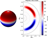 |
Fig. 1. Magnetic field model located at the base of the convection zone with Bmax = 300 kG, μ = 0.713 R⊙, σ = 0.05 R⊙ and harmonic degree s = 2. The right-hand side shows the radial and co-latitudinal distribution, while the left-hand side emphasises the longitudinal symmetry. |
Modes are affected by the direct effect of the toroidal magnetic field only if they pass through the layers where the field is present. The modes must penetrate at least to rthresh = 0.863 R⊙ to be within 3σ of the magnetic field distribution. The P-modes are confined between a lower turning point rt and the surface. The lower turning point rt for p-modes is located where the frequency is equal to the Lamb frequency, ω = Sl(rt). This gives
 (63)
(63)
Multiplets with lower turning points larger than rthresh are expected to exhibit negligible frequency shifts. Therefore, we excluded multiplets with rt > rthresh from this study. This is particularly true for multiplets with l ≥ 138.
5. Results
We computed the frequency shifts in a solar model caused by the direct effect of a toroidal magnetic field located at the base of the convection zone for modes up to 5200 μHz in the range 2 ≤ l ≤ 137. We excluded modes with l ≥ 138, since their lower turning points lie outside the region where the toroidal magnetic field is significant. For each degenerate multiplet ω0, x2 we constructed an eigenspace Kx around ωref2 = ω0, x2. Contributions from multiplets with frequency gaps larger than about 0.1 μHz are negligible compared to the self-coupling terms. Based on this, we chose an eigenspace width of  Hz2.
Hz2.
Figure 2 shows the m-averaged frequency shifts as a function of the unperturbed multiplet frequencies. Multiplets with the same harmonic degree l are connected. The overall form of the shifts matches those obtained by Kiefer & Roth (2018) (cf. Figure 3 therein), but their magnitudes, reaching up to 14 nHz, are about twice as large in our study. All multiplets show a positive frequency shift.
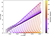 |
Fig. 2. Multiplet frequency shifts, averaged over m, as a function of their unperturbed mode frequencies. Multiplets with the same harmonic degree l are connected. |
Figure 3 presents the m-averaged frequency shifts as a function of the lower turning point rt. The vertical line marks the radius rthresh = 0.863 R⊙, beyond which modes are expected to be unaffected by the direct effect of the toroidal magnetic field. As rt approaches rthresh, the frequency shifts of the modes tend to zero. Modes with rt above rthresh propagate outside of the magnetised regions, where they experience negligible shifts due to the direct effect of the magnetic field. This can be confirmed by examining the radial contributions in Equation (50). Multiplets with turning points near the maximum of the magnetic field distribution exhibit the greatest frequency shift. The shifts decrease for multiplets with lower turning points beyond the location of the maximum field strength.
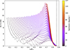 |
Fig. 3. Multiplet frequency shifts, averaged over m, as a function of their lower turning point. Multiplets with the same harmonic degree l are connected. The dashed vertical line indicates the threshold radius rthresh = 0.863 R⊙, above which modes are not affected by the magnetic field. |
Figure 4 displays the lifting of the degeneracy of the multiplet frequency with respect to the azimuthal order m. The absolute frequency shift of the multiplet modes is plotted against m/l and the harmonic degree l. The colour code indicates the radial order n. The degeneracy in m of the unperturbed multiplet is not completely lifted by the interaction with the toroidal magnetic field. Modes within a multiplet remain degenerate if they have the same absolute value of m. This is a result of the symmetry in the angular kernels under the exchange of m ↔ −m, assuming selection rule (59) is fulfilled. The symmetry of the angular kernels is verifiable using Equations (D.1), (D.5), and (D.16). For all multiplets with l ≥ 53 and n ≥ 9, the frequency shift reaches its maximum at m = 0 and decreases monotonically on both sides, approaching zero at |m|=l. For harmonic degrees l ≥ 65, the frequency shift at a fixed m/l increases with radial order n. The mode m = 0, l = 69, n = 19 exhibits the maximum frequency shift within the considered mode range. The plateau of the largest frequency shifts for m = 0 modes aligns with multiplets having lower turning points near the maximum of the magnetic field distribution at μ = 0.713 R⊙. For multiplets with l ≳ 80, the frequency shift magnitude decreases sharply due to their higher lower turning points. For multiplets with l < 53, only those with intermediate radial order n display a maximum shift at m = 0. The number of multiplets with l < 53 that exhibit this behaviour decreases with decreasing l. For modes in other multiplets, the frequency shifts exhibit a local minimum at m = 0 and two maxima.
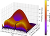 |
Fig. 4. Frequency shifts of m-resolved multiplet modes as a function of m/l and l. The colour represents the radial order n. |
6. Discussion and conclusion
Our calculations refine the results of Kiefer et al. (2017) and Kiefer & Roth (2018). While our corrected analysis produces quantitative differences, the qualitative trends and conclusions largely align with their findings. The theory presented here is also applicable to stellar models.
A toroidal magnetic field in the stellar interior couples stellar oscillation eigenmodes and partially lifts the degeneracy of the multiplet frequencies. The general matrix element between two modes quantifies their coupling strength. In this study, we present a revised expression of the general matrix element for the direct effect due to a toroidal magnetic field. Equation (50) is used for forward calculations of the direct effect of a strong toroidal field located at the base of the convection zone. The presented theory enables an investigation of the direct effect of subsurface toroidal magnetic field distributions on stellar oscillation frequencies. We obtained frequency shifts to the oscillation modes by computing the eigenvalues and eigenvectors of the supermatrix following the quasi-degenerate perturbation theory (Lavely & Ritzwoller 1992). Only modes with the same azimuthal order can couple through the toroidal magnetic field (Equation (59)). In addition, the sum of the harmonic degrees of the coupling modes and the toroidal magnetic field components must be even (Equation (61)).
We found that previous studies omit non-zero contributions when calculating integrals over products of scalar GSHs. To address this, we derived a complete method for computing such integrals. The general solution for these integrals, which also includes cases where N1 ≠ ∑i > 1Ni, is applicable outside helioseismology, for example in the addition of angular momentum in quantum dynamics.
This study does not include the indirect effect, which represents changes in the equilibrium structure induced by the magnetic field. For magnetic models with s = 2, the indirect effect on the mean multiplet shift is much smaller than the direct effect and can be neglected (Kiefer & Roth 2018). However, a complete description of the frequency perturbations requires its inclusion. Detailed computations of the indirect effect are provided by Kiefer & Roth (2018). The reported absolute values of the indirect effect are likely underestimated because Kiefer & Roth (2018) assumes that integrals with N1 ≠ ∑i > 1Ni, which are involved in the computation, vanish. This assumption leads to the neglect of non-zero contributions.
For a strong magnetic field distribution located at the base of the solar convection zone, the m-averaged shift of the multiplet frequencies is of the order of tens of nanohertz. Although this shift is nearly twice that obtained for the same magnetic field model by Kiefer & Roth (2018), it still does not explain the observed frequency shifts over a solar cycle. Broomhall (2017) measured the shift between the maximum and the minimum of solar cycle 23 using data from the Global Oscillation Network Group (GONG). These shifts are of the order of several hundred nanohertz up to microhertz. Hence, near-surface magnetic fields are likely responsible for the observed frequency shifts. However, the existence of deep magnetic field distributions cannot be ruled out. The detection of such fields is strongly hampered, as effects of near-surface fields are stronger by orders of magnitude. The case of the Sun thus differs from that of evolved stars, where a deep fossil field in the stellar core may strongly affect stellar oscillations (Fuller et al. 2015; Bugnet et al. 2021).
The recent study by Vasil et al. (2024), based on magnetohydrodynamic simulations, contributes to the discussion of whether the solar dynamo operates solely near the solar surface. Further studies on the effects of near-surface magnetic fields on oscillations are therefore of particular interest. For this purpose, the solar model should be extended to include an atmosphere. The refined theory is expected to yield significantly different constraints on the model parameters of a near-surface magnetic field that reproduce the observed shifts of Broomhall (2017), compared to those provided by Kiefer & Roth (2018).
Kiefer & Roth (2018) conclude that plotting observed frequency shifts as a function of their lower turning point, as shown in Figure 3, provides hints about the location of the magnetic field configuration. The location of a local maximum in the magnetic field strength can be inferred from the lower turning points of multiplets, whose shifts begin to decline monotonically at a specific harmonic degree. However, the superposition of differently located magnetic field components can hamper such conclusions, since deeper fields produce smaller shifts even if they are stronger than near-surface fields. The revised calculations, which yield larger frequency shifts, combined with sufficient observational resolution, could facilitate identifying dips in such plots that indicate local field maxima.
This work provides a refined analytical solution for the direct effect of a toroidal magnetic field, potentially serving as a stepping stone towards inversion techniques for solar and stellar magnetic field studies. The solution facilitates more detailed studies and tighter constraints on the location of solar and stellar dynamos. Furthermore, we developed a computational framework implementing the quasi-degenerate perturbation theory for a toroidal magnetic field, enabling precise calculations of supermatrices and frequency shifts. This extends its applicability to a wide range of astrophysical scenarios, including different stellar models and magnetic field configurations. For example, it allows parametric studies of detectability thresholds of magnetic field configurations in the Sun and other stars above the measurement noises of related instruments for helio- and asteroseismology (e.g. GONG, HMI, Kepler, TESS, and PLATO). The code is publicly available on GitHub1, promoting transparency and encouraging community collaboration in future research.
Acknowledgments
The authors thank René Kiefer for fruitful discussions. We thank the anonymous referee for valuable comments that improved the manuscript.
References
- Aerts, C., Christensen-Dalsgaard, J., & Kurtz, D. W. 2010, Asteroseismology (Dordrecht: Springer) [Google Scholar]
- Antia, H. M., Chitre, S. M., & Thompson, M. J. 2000, A&A, 360, 335 [NASA ADS] [Google Scholar]
- Antia, H. M., Chitre, S. M., & Gough, D. O. 2013, MNRAS, 428, 470 [Google Scholar]
- Arfken, G. B., Weber, H. J., & Harris, F. E. 2012, Mathematical Methods for Physicists: A Comprehensive Guide, 7th edn. (Boston, MA, USA: Academic Press) [Google Scholar]
- Baldner, C. S., Antia, H. M., Basu, S., & Larson, T. P. 2009, ApJ, 705, 1704 [NASA ADS] [CrossRef] [Google Scholar]
- Basu, S., Antia, H. M., & Tripathy, S. C. 1999, ApJ, 512, 458 [Google Scholar]
- Bernstein, I. B., Frieman, E. A., Kruskal, M. D., & Kulsrud, R. M. 1958, Proc. R. Soc. London Ser. A, 244, 17 [Google Scholar]
- Bhattacharya, S., Das, S. B., Bugnet, L., Panda, S., & Hanasoge, S. M. 2024, ApJ, 970, 42 [NASA ADS] [CrossRef] [Google Scholar]
- Braithwaite, J., & Spruit, H. C. 2004, Nature, 431, 819 [Google Scholar]
- Braun, D. C. 2019, ApJ, 873, 94 [NASA ADS] [CrossRef] [Google Scholar]
- Broomhall, A. M. 2017, Sol. Phys., 292, 67 [Google Scholar]
- Bugnet, L., Prat, V., Mathis, S., et al. 2021, A&A, 650, A53 [NASA ADS] [CrossRef] [EDP Sciences] [Google Scholar]
- Cally, P. S. 2000, Sol. Phys., 192, 395 [Google Scholar]
- Chandrasekhar, S. 1964, ApJ, 139, 664 [Google Scholar]
- Charbonneau, P. 2020, Liv. Rev. Sol. Phys., 17, 4 [Google Scholar]
- Christensen-Dalsgaard, J. 2002, Rev. Mod. Phys., 74, 1073 [Google Scholar]
- Christensen-Dalsgaard, J., Dappen, W., Ajukov, S. V., et al. 1996, Science, 272, 1286 [Google Scholar]
- Dahlen, F. A., & Tromp, J. 1998, Theoretical Global Seismology (Princeton University Press) [Google Scholar]
- Das, S. B., Chakraborty, T., Hanasoge, S. M., & Tromp, J. 2020, ApJ, 897, 38 [NASA ADS] [CrossRef] [Google Scholar]
- Das, S. B., Einramhof, L., & Bugnet, L. 2024, A&A, 690, A217 [NASA ADS] [CrossRef] [EDP Sciences] [Google Scholar]
- Dong, S.-H., & Lemus, R. 2002, Appl. Math. Lett., 15, 541 [CrossRef] [Google Scholar]
- Duez, V., & Mathis, S. 2010, A&A, 517, A58 [NASA ADS] [CrossRef] [EDP Sciences] [Google Scholar]
- Duvall, T. L., Jr, Jefferies, S. M., Harvey, J. W., & Pomerantz, M. A. 1993, Nature, 362, 430 [Google Scholar]
- Dziembowski, W. A., & Goode, P. R. 1991, ApJ, 376, 782 [Google Scholar]
- Dziembowski, W. A., & Goode, P. R. 2004, ApJ, 600, 464 [Google Scholar]
- Edmonds, A. R. 1960, Angular Momentum in Quantum Mechanics (Princeton University Press) [Google Scholar]
- Fan, Y. 2009, Liv. Rev. Sol. Phys., 6, 4 [Google Scholar]
- Fan, Y. 2021, Liv. Rev. Sol. Phys., 18, 5 [NASA ADS] [CrossRef] [Google Scholar]
- Fuller, J., Cantiello, M., Stello, D., Garcia, R. A., & Bildsten, L. 2015, Science, 350, 423 [Google Scholar]
- Giles, P. M. 2000, Ph.D. Thesis, Stanford University, California, [Google Scholar]
- Gizon, L., Schunker, H., Baldner, C. S., et al. 2009, Space Sci. Rev., 144, 249 [Google Scholar]
- Goedbloed, J. H., & Poedts, S. 2004, Principles of magnetohydrodynamics: with applications to laboratory and astrophysical plasmas (Cambridge University Press) [Google Scholar]
- Gough, D. O., & Thompson, M. J. 1990, MNRAS, 242, 25 [Google Scholar]
- Hanasoge, S. M. 2017, MNRAS, 470, 2780 [Google Scholar]
- Hanasoge, S., Birch, A., Gizon, L., & Tromp, J. 2012, Phys. Rev. Lett., 109, 101101 [Google Scholar]
- Hanasoge, S. M., Woodard, M., Antia, H. M., Gizon, L., & Sreenivasan, K. R. 2017, MNRAS, 470, 1404 [Google Scholar]
- Hathaway, D. H. 2015, Liv. Rev. Sol. Phys., 12, 4 [Google Scholar]
- Hill, F. 1988, ApJ, 333, 996 [Google Scholar]
- Jermyn, A. S., Bauer, E. B., Schwab, J., et al. 2023, ApJS, 265, 15 [NASA ADS] [CrossRef] [Google Scholar]
- Khomenko, E., & Collados, M. 2015, Liv. Rev. Sol. Phys., 12, 6 [Google Scholar]
- Kiefer, R., & Roth, M. 2018, ApJ, 854, 74 [Google Scholar]
- Kiefer, R., Schad, A., & Roth, M. 2017, ApJ, 846, 162 [Google Scholar]
- Lavely, E. M., & Ritzwoller, M. H. 1992, Phil. Trans. R. Soc. London Ser. A, 339, 431 [Google Scholar]
- Leighton, R. B., Noyes, R. W., & Simon, G. W. 1962, ApJ, 135, 474 [NASA ADS] [CrossRef] [Google Scholar]
- Li, G., Deheuvels, S., Li, T., Ballot, J., & Lignières, F. 2023, A&A, 680, A26 [NASA ADS] [CrossRef] [EDP Sciences] [Google Scholar]
- Loi, S. T. 2020, MNRAS, 496, 3829 [Google Scholar]
- Lynden-Bell, D., & Ostriker, J. P. 1967, MNRAS, 136, 293 [Google Scholar]
- Masters, G., & Richards-Dinger, K. 1998, Geophys. J. Int., 135, 307 [Google Scholar]
- Mathis, S., & de Brye, N. 2011, A&A, 526, A65 [CrossRef] [EDP Sciences] [Google Scholar]
- Miesch, M. S. 2005, Liv. Rev. Sol. Phys., 2, 1 [Google Scholar]
- Ossendrijver, M. 2003, A&ARv, 11, 287 [Google Scholar]
- Paxton, B., Bildsten, L., Dotter, A., et al. 2011, ApJS, 192, 3 [Google Scholar]
- Paxton, B., Cantiello, M., Arras, P., et al. 2013, ApJS, 208, 4 [Google Scholar]
- Paxton, B., Marchant, P., Schwab, J., et al. 2015, ApJS, 220, 15 [Google Scholar]
- Paxton, B., Schwab, J., Bauer, E. B., et al. 2018, ApJS, 234, 34 [NASA ADS] [CrossRef] [Google Scholar]
- Paxton, B., Smolec, R., Schwab, J., et al. 2019, ApJS, 243, 10 [Google Scholar]
- Phinney, R. A., & Burridge, R. 1973, Geophys. J., 34, 451 [CrossRef] [Google Scholar]
- Prat, V., Mathis, S., Buysschaert, B., et al. 2019, A&A, 627, A64 [NASA ADS] [CrossRef] [EDP Sciences] [Google Scholar]
- Press, W. H., Teukolsky, S. A., Vetterling, W. T., & Flannery, B. P. 2007, Numerical Recipes: The Art of Scientific Computing, 3rd edn. (Cambridge, New York, Melbourne, Madrid, Cape Town, Singapore, São Paulo: Cambridge University Press) [Google Scholar]
- Rabello-Soares, M. C., Bogart, R. S., & Scherrer, P. H. 2018, ApJ, 859, 7 [Google Scholar]
- Racah, G. 1942, Phys. Rev., 62, 438 [NASA ADS] [CrossRef] [Google Scholar]
- Ritzwoller, M. H., & Lavely, E. M. 1991, ApJ, 369, 557 [CrossRef] [Google Scholar]
- Roth, M. 2002, Ph.D. Thesis, Albert Ludwigs University of Freiburg, Germany [Google Scholar]
- Roth, M., & Stix, M. 2008, Sol. Phys., 251, 77 [Google Scholar]
- Schou, J., Christensen-Dalsgaard, J., & Thompson, M. J. 1994, ApJ, 433, 389 [NASA ADS] [CrossRef] [Google Scholar]
- Schunker, H., & Cally, P. S. 2006, MNRAS, 372, 551 [Google Scholar]
- Sekii, T. 1990, in Progress of Seismology of the Sun and Stars, eds. Y. Osaki, & H. Shibahashi, 367, 337 [Google Scholar]
- Sekii, T. 1991, PASJ, 43, 381 [Google Scholar]
- Stello, D., Cantiello, M., Fuller, J., et al. 2016, Nature, 529, 364 [Google Scholar]
- Townsend, R. H. D., & Teitler, S. A. 2013, MNRAS, 435, 3406 [Google Scholar]
- Townsend, R. H. D., Goldstein, J., & Zweibel, E. G. 2018, MNRAS, 475, 879 [Google Scholar]
- Unno, W., Osaki, Y., Ando, H., Saio, H., & Shibahashi, H. 1989, Nonradial oscillations of stars (University of Tokyo Press) [Google Scholar]
- Vasil, G. M., Lecoanet, D., Augustson, K., et al. 2024, Nature, 629, 769 [CrossRef] [Google Scholar]
- Weiss, N. O., Brownjohn, D. P., Matthews, P. C., & Proctor, M. R. E. 1996, MNRAS, 283, 1153 [Google Scholar]
- Woodard, M. F., & Noyes, R. W. 1988, in Advances in Helio- and Asteroseismology (Dordrecht, Netherlands: Springer), 197 [Google Scholar]
- Zhao, J., & Kosovichev, A. G. 2004, ApJ, 603, 776 [Google Scholar]
Appendix A: Mathematical auxiliaries
This appendix lists the vector identities and formulae used to calculate the general matrix element for a toroidal magnetic field described by equation (50). The calculations use spherical coordinates with radius r, co-latitude θ, and azimuthal angle ϕ.
Here, A(r, θ, ϕ) and B(r, θ, ϕ) denote general vector fields. The curl of the cross-product of two vector fields A and B is given by:
 (A.1)
(A.1)
The divergence of a vector field A in spherical coordinates is given by:
 (A.2)
(A.2)
and its curl is:
 (A.3)
(A.3)
The gradient of a scalar field f(r, θ, ϕ) in spherical coordinates is expressed as:
 (A.4)
(A.4)
The Laplace operator of a scalar field f in spherical coordinates is defined by:
 (A.5)
(A.5)
The material derivative of the vector fields A and B in spherical coordinates can be computed as:
 (A.6)
(A.6)
Appendix B: Perturbation operator of direct effect and calculation of general matrix element
Section 4 presents the general matrix element for the direct effect of a toroidal magnetic field. This appendix outlines the derivation of the general matrix element and provides an explicit expression for the perturbation operator.
Using the mathematical tools described in Appendix A, the operator for a toroidal magnetic field perturbation ℱB(ξ0, k), is derived for fixed values of s and s′ through a straightforward but lengthy calculation. For clarity, the eigenfunctions are represented as follows:
 (B.1)
(B.1)
The first expressions for the magnetic field components (46) and (47), along with the representation of the eigenfunctions (B.1), are substituted into the magnetic field perturbation operator (17), leading to the following result:
![Mathematical equation: $$ \begin{aligned}&{\mathcal{F} }_B(\boldsymbol{\xi }_{0,k}) = -\frac{1}{4\pi \rho _0}\Bigg [\bigg \{\frac{( \boldsymbol{\xi }_{0,k}\cdot \nabla ) \rho _0}{\rho _0}+\nabla \cdot \boldsymbol{\xi }_{0,k}\bigg \}\big (\nabla \times \mathbf B _s\big ) \times \mathbf B _{s^{\prime }} \nonumber \\&+\big (\nabla \times \mathbf B _s\big ) \times \Big \{ \nabla \times \big (\boldsymbol{\xi }_{0,k} \times \mathbf B _{s^{\prime }}\big )\Big \} +\bigg (\nabla \times \Big \{ \nabla \times \big (\boldsymbol{\xi }_{0,k} \times \mathbf B _s\big )\Big \}\bigg ) \times \mathbf B _{s^{\prime }}\Bigg ] \nonumber \\&=\ \frac{1}{4\pi \rho _0}{[}\Biggl \{\bigg (\frac{B_\phi \tilde{B}_\phi \xi ^r}{r}\frac{\partial {\ln \rho _0}}{\partial {r}}+\tilde{B}_\phi \xi ^r\frac{\partial {\ln \rho _0}}{\partial {r}}\frac{\partial {B_\phi }}{\partial {r}}\bigg )\hat{\mathbf{e }}_r +\bigg (\frac{B_\phi \tilde{B}_\phi \xi ^r\cot \theta }{r} \nonumber \\&\quad \cdot \frac{\partial {\ln \rho _0}}{\partial {r}} +\frac{\tilde{B}_\phi \xi ^r}{r}\frac{\partial {\ln \rho _0}}{\partial {r}}\frac{\partial {B_\phi }}{\partial {\theta }}\bigg )\hat{\mathbf{e }}_\theta \Biggr \}+\Bigg \{\bigg (\frac{2B_\phi \tilde{B}_\phi \xi ^r}{r^2}+\frac{B_\phi \tilde{B}_\phi \xi ^\theta \cot \theta }{r^2} \nonumber \\&\quad +\frac{B_\phi \tilde{B}_\phi }{r}\frac{\partial {\xi ^r}}{\partial {r}} +\frac{B_\phi \tilde{B}_\phi }{r^2}\frac{\partial {\xi ^\theta }}{\partial {\theta }}+\frac{B_\phi \tilde{B}_\phi }{r^2\sin \theta }\frac{\partial {\xi ^\phi }}{\partial {\phi }} +\frac{2\tilde{B}_\phi \xi ^r}{r}\frac{\partial {B_\phi }}{\partial {r}}\nonumber \\&\quad +\frac{\tilde{B}_\phi \xi ^\theta \cot \theta }{r}\frac{\partial {B_\phi }}{\partial {r}}+\tilde{B}_\phi \frac{\partial {\xi ^r}}{\partial {r}}\frac{\partial {B_\phi }}{\partial {r}} +\frac{\tilde{B}_\phi }{r}\frac{\partial {\xi ^\theta }}{\partial {\theta }}\frac{\partial {B_\phi }}{\partial {r}}+\frac{\tilde{B}_\phi }{r\sin \theta }\frac{\partial {\xi ^\phi }}{\partial {\phi }} \nonumber \\&\quad \cdot \frac{\partial {B_\phi }}{\partial {r}}\bigg )\hat{\mathbf{e }}_r+\bigg (\frac{2B_\phi \tilde{B}_\phi \xi ^r\cot \theta }{r^2}+\frac{B_\phi \tilde{B}_\phi \xi ^\theta \cot ^2\theta }{r^2}+\frac{B_\phi \tilde{B}_\phi \cot \theta }{r}\frac{\partial {\xi ^r}}{\partial {r}} \nonumber \\&\quad +\frac{B_\phi \tilde{B}_\phi \cot \theta }{r^2}\frac{\partial {\xi ^\theta }}{\partial {\theta }}+\frac{B_\phi \tilde{B}_\phi \cot \theta }{r^2\sin \theta }\frac{\partial {\xi ^\phi }}{\partial {\phi }} +\frac{2\tilde{B}_\phi \xi ^r}{r^2}\frac{\partial {B_\phi }}{\partial {\theta }}+\frac{\tilde{B}_\phi \xi ^\theta \cot \theta }{r^2} \nonumber \\&\quad \cdot \frac{\partial {B_\phi }}{\partial {\theta }}+\frac{\tilde{B}_\phi }{r}\frac{\partial {\xi ^r}}{\partial {r}}\frac{\partial {B_\phi }}{\partial {\theta }}+\frac{\tilde{B}_\phi }{r^2}\frac{\partial {\xi ^\theta }}{\partial {\theta }}\frac{\partial {B_\phi }}{\partial {\theta }}+\frac{\tilde{B}_\phi }{r^2\sin \theta }\frac{\partial {\xi ^\phi }}{\partial {\phi }}\frac{\partial {B_\phi }}{\partial {\theta }}\bigg )\hat{\mathbf{e }}_\theta \Bigg \} \nonumber \\&\quad -\Bigg \{\bigg (\frac{B_\phi \tilde{B}_\phi \xi ^r}{r^2}+\frac{B_\phi \tilde{B}_\phi }{r}\frac{\partial {\xi ^r}}{\partial {r}}+\frac{B_\phi \tilde{B}_\phi }{r^2}\frac{\partial {\xi ^\theta }}{\partial {\theta }}+\frac{\tilde{B}_\phi \xi ^r}{r}\frac{\partial {B_\phi }}{\partial {r}}+\frac{B_\phi \xi ^r}{r}\frac{\partial {\tilde{B}_\phi }}{\partial {r}} \nonumber \\&\quad +\frac{B_\phi \xi ^\theta }{r^2}\frac{\partial {\tilde{B}_\phi }}{\partial {\theta }} +\tilde{B}_\phi \frac{\partial {\xi ^r}}{\partial {r}}\frac{\partial {B_\phi }}{\partial {r}}+\frac{\tilde{B}_\phi }{r}\frac{\partial {\xi ^\theta }}{\partial {\theta }}\frac{\partial {B_\phi }}{\partial {r}}+\xi ^r\frac{\partial {B_\phi }}{\partial {r}}\frac{\partial {\tilde{B}_\phi }}{\partial {r}}+\frac{\xi ^\theta }{r} \nonumber \\&\quad \cdot \frac{\partial {B_\phi }}{\partial {r}}\frac{\partial {\tilde{B}_\phi }}{\partial {\theta }}\bigg )\hat{\mathbf{e }}_r +\bigg (\frac{B_\phi \tilde{B}_\phi \xi ^r\cot \theta }{r^2}+\frac{B_\phi \tilde{B}_\phi \cot \theta }{r}\frac{\partial {\xi ^r}}{\partial {r}}+\frac{B_\phi \tilde{B}_\phi \cot \theta }{r^2} \nonumber \\&\quad \cdot \frac{\partial {\xi ^\theta }}{\partial {\theta }}+\frac{B_\phi \xi ^r\cot \theta }{r}\frac{\partial {\tilde{B}_\phi }}{\partial {r}} +\frac{B_\phi \xi ^\theta \cot \theta }{r^2}\frac{\partial {\tilde{B}_\phi }}{\partial {\theta }} +\frac{\tilde{B}_\phi \xi ^r}{r^2}\frac{\partial {B_\phi }}{\partial {\theta }}+\frac{\tilde{B}_\phi }{r}\frac{\partial {\xi ^r}}{\partial {r}} \nonumber \\&\quad \cdot \frac{\partial {B_\phi }}{\partial {\theta }}+\frac{\tilde{B}_\phi }{r^2}\frac{\partial {\xi ^\theta }}{\partial {\theta }}\frac{\partial {B_\phi }}{\partial {\theta }}+\frac{\xi ^r}{r}\frac{\partial {\tilde{B}_\phi }}{\partial {r}}\frac{\partial {B_\phi }}{\partial {\theta }} +\frac{\xi ^\theta }{r^2}\frac{\partial {\tilde{B}_\phi }}{\partial {\theta }}\frac{\partial {B_\phi }}{\partial {\theta }}\bigg )\hat{\mathbf{e }}_\theta \nonumber \\&\quad +\bigg (\frac{B_\phi \tilde{B}_\phi }{r^2\sin \theta }\frac{\partial {\xi ^r}}{\partial {\phi }}+\frac{B_\phi \tilde{B}_\phi \cot \theta }{r^2\sin \theta }\frac{\partial {\xi ^\theta }}{\partial {\phi }}+\frac{\tilde{B}_\phi }{r\sin \theta }\frac{\partial {\xi ^r}}{\partial {\phi }}\frac{\partial {B_\phi }}{\partial {r}} +\frac{\tilde{B}_\phi }{r^2\sin \theta } \nonumber \\&\quad \cdot \frac{\partial {\xi ^\theta }}{\partial {\phi }}\frac{\partial {B_\phi }}{\partial {\theta }}\bigg )\hat{\mathbf{e }}_\phi \Bigg \} -\Bigg \{\bigg (\frac{2B_\phi \tilde{B}_\phi }{r}\frac{\partial {\xi ^r}}{\partial {r}}+\frac{2\tilde{B}_\phi \xi ^r}{r}\frac{\partial {B_\phi }}{\partial {r}}+B_\phi \tilde{B}_\phi \frac{\partial {^2\xi ^r}}{\partial {r^2}} \nonumber \\&\quad +\frac{B_\phi \tilde{B}_\phi }{r^2\sin ^2\theta }\frac{\partial {^2\xi ^r}}{\partial {\phi ^2}}+\frac{B_\phi \tilde{B}_\phi }{r}\frac{\partial {^2\xi ^\theta }}{\partial {r\partial \theta }} +2\tilde{B}_\phi \frac{\partial {\xi ^r}}{\partial {r}}\frac{\partial {B_\phi }}{\partial {r}}+\frac{\tilde{B}_\phi }{r}\frac{\partial {\xi ^\theta }}{\partial {\theta }}\frac{\partial {B_\phi }}{\partial {r}} \nonumber \\&\quad +\frac{\tilde{B}_\phi }{r}\frac{\partial {\xi ^\theta }}{\partial {r}}\frac{\partial {B_\phi }}{\partial {\theta }} +\xi ^r\tilde{B}_\phi \frac{\partial {^2B_\phi }}{\partial {r^2}}+\frac{\tilde{B}_\phi \xi ^\theta }{r}\frac{\partial {^2B_\phi }}{\partial {r\partial \theta }}\bigg )\hat{\mathbf{e }}_r +\bigg (\frac{B_\phi \tilde{B}_\phi \xi ^r\cot \theta }{r^2} \nonumber \\&\quad +\frac{B_\phi \tilde{B}_\phi }{r^2}\frac{\partial {\xi ^r}}{\partial {\theta }}+\frac{B_\phi \tilde{B}_\phi \cot \theta }{r}\frac{\partial {\xi ^r}}{\partial {r}} +\frac{B_\phi \tilde{B}_\phi \cot \theta }{r^2}\frac{\partial {\xi ^\theta }}{\partial {\theta }}+\frac{\tilde{B}_\phi \xi ^r\cot \theta }{r} \nonumber \\&\quad \cdot \frac{\partial {B_\phi }}{\partial {r}}+\frac{\tilde{B}_\phi \xi ^r}{r^2}\frac{\partial {B_\phi }}{\partial {\theta }}+\frac{\tilde{B}_\phi \xi ^\theta \cot \theta }{r^2}\frac{\partial {B_\phi }}{\partial {\theta }}+\frac{B_\phi \tilde{B}_\phi }{r^2}\frac{\partial {^2\xi ^\theta }}{\partial {\theta ^2}} +\frac{B_\phi \tilde{B}_\phi }{r^2\sin ^2\theta } \nonumber \\&\quad \cdot \frac{\partial {^2\xi ^\theta }}{\partial {\phi ^2}}+\frac{B_\phi \tilde{B}_\phi }{r}\frac{\partial {^2\xi ^r}}{\partial {r\partial \theta }}+\frac{\tilde{B}_\phi }{r}\frac{\partial {\xi ^r}}{\partial {r}}\frac{\partial {B_\phi }}{\partial {\theta }}+\frac{2\tilde{B}_\phi }{r^2}\frac{\partial {\xi ^\theta }}{\partial {\theta }}\frac{\partial {B_\phi }}{\partial {\theta }}+\frac{\tilde{B}_\phi }{r}\frac{\partial {\xi ^r}}{\partial {\theta }} \nonumber \\&\quad \cdot \frac{\partial {B_\phi }}{\partial {r}}+\frac{\tilde{B}_\phi \xi ^\theta }{r^2}\frac{\partial {^2B_\phi }}{\partial {\theta ^2}}+\frac{\tilde{B}_\phi \xi ^r}{r}\frac{\partial {^2B_\phi }}{\partial {r\partial \theta }}\bigg )\hat{\mathbf{e }}_\theta \Bigg \}{]} \ . \end{aligned} $$](/articles/aa/full_html/2026/03/aa54413-25/aa54413-25-eq94.gif) (B.2)
(B.2)
The four terms in the first equality are kept separate and enclosed within curly brackets. The left scalar product of equation (B.2) with ρ0ξ0, k′* is computed and integrated over the entire stellar volume. Subsequently, the second expressions from equations (46), (47), and (B.1) are inserted, using the notation for the complex conjugated eigenfunctions given in (49). Finally, sorting by the angular kernels S1 – S23, as defined in equations (G.1) – (G.23) in Appendix G, results in the general matrix element for the direct effect of a toroidal magnetic field, given in equation (50).
Appendix C: Restoration of hermiticity in the total force operator
In this appendix, we demonstrate that our full force operator, defined in equation (16), reduces to the expression given in equation (6.23) of Goedbloed & Poedts (2004). We note that Goedbloed & Poedts (2004) used a magnetised equilibrium, did not include perturbations of the gravitational potential, and did not use cgs units.
We begin by rewriting the first term of the operator of the direct magnetic effect ℱB, presented in equation (17), as:
 (C.1)
(C.1)
Here, we used the magnetised equilibrium condition (14) to eliminate the term containing the equilibrium magnetic field. We also applied the product rule for divergence:
 (C.2)
(C.2)
and the linearised continuity equation (e.g., Lynden-Bell & Ostriker 1967; Christensen-Dalsgaard 2002; Goedbloed & Poedts 2004):
 (C.3)
(C.3)
We can express the modified equilibrium operator  as:
as:
 (C.4)
(C.4)
 (C.5)
(C.5)
where we used equation (C.3) and the linearised energy equation (e.g., Lynden-Bell & Ostriker 1967; Christensen-Dalsgaard 2002; Goedbloed & Poedts 2004):
 (C.6)
(C.6)
Plugging equation (C.1) into the expression for ℱB given in equation (17) and summing it with  yields:
 (C.7)
(C.7)
This is equivalent to  , where FGP is given in equation (6.23) of Goedbloed & Poedts (2004), except that we applied the linearised continuity equation and perturbed the gravitational potential resulting in an additional ∇ϕ′ term.
Next, we explicitly identify where the Hermiticity breaks down in ℱB and find the symmetric partners in  . We use the inner product:
 (C.8)
(C.8)
where η, ξ are two displacement fields. To simplify the proof and follow the formalism of Goedbloed & Poedts (2004) more closely, we assumed fixed boundary conditions:
 (C.9)
(C.9)
where n is the normal vector of the surface. Under these boundary conditions, surface integrals vanish; these are equivalent to the volume integrals of divergence terms after applying the Gauss-divergence theorem. For the zero-boundary conditions (Unno et al. 1989) discussed in Section 2.1, the surface terms do not vanish but instead form a symmetric boundary energy term (Bernstein et al. 1958; Lynden-Bell & Ostriker 1967). Therefore, Hermiticity is preserved even when ξ ⋅ n ≠ 0. We split ℱB(ξ) into three parts:
 (C.10)
 (C.11)
 (C.12)
where in the last operator we applied equation (C.1). Goedbloed & Poedts (2004) show that  and the second pressure term
  form symmetric expressions plus divergence terms, which can be discarded upon integration due to the boundary condition (C.9). We can also show explicitly that the work done by the perturbed gravitational field is Hermitian:
![Mathematical equation: $$ \begin{aligned} -\int _{V}\boldsymbol{\eta }^{*}\cdot \boldsymbol{g}^{\prime }(\boldsymbol{\xi })\tilde{\rho }_0\mathrm{d} V=&\int _{V}\boldsymbol{\eta }^{*}\cdot \nabla \phi ^{\prime }[\boldsymbol{\xi }]\tilde{\rho }_0\mathrm{d} V \nonumber \\ \overset{{(\mathrm{C.2})}}{=}&\int _{V}\nabla \cdot (\boldsymbol{\eta }^{*}\phi ^{\prime }[\boldsymbol{\xi }]\tilde{\rho }_0)\mathrm{d} V \nonumber \\&-\int _{V}\phi ^{\prime }[\boldsymbol{\xi }]\nabla \cdot (\tilde{\rho }_0\boldsymbol{\eta }^{*})\mathrm{d} V \ , \end{aligned} $$](/articles/aa/full_html/2026/03/aa54413-25/aa54413-25-eq113.gif) (C.13)
(C.13)
where we used g′(ξ) = − ∇ϕ′[ξ] in the first equality. The first integral in the last equation is again a vanishing boundary term. Using the continuity equation in the form ![Mathematical equation: $ \rho\prime[\boldsymbol{\eta}^{\ast}]=-\nabla\cdot(\tilde{\rho}_0\boldsymbol{\eta}^{\ast}) $](/articles/aa/full_html/2026/03/aa54413-25/aa54413-25-eq114.gif) and the Poisson equation ∇2ϕ′ = 4πGρ′, we get:
and the Poisson equation ∇2ϕ′ = 4πGρ′, we get:
![Mathematical equation: $$ \begin{aligned} -\int _{V}\boldsymbol{\eta }^*\cdot \boldsymbol{g}^{\prime }(\boldsymbol{\xi })\rho _0\mathrm{d} V=&\int _{V}\phi ^{\prime }[\boldsymbol{\xi }]\rho ^{\prime }[\boldsymbol{\eta ^{*}}]\mathrm{d} V \nonumber \\ =&\frac{1}{4\pi G}\int _{V}\phi ^{\prime }[\boldsymbol{\xi }]\nabla ^2\phi ^{\prime }[\boldsymbol{\eta ^{*}}]\mathrm{d} V \nonumber \\ \overset{{(\mathrm{C.2})}}{=}&\frac{1}{4\pi G}\bigg [\int _{V}\nabla \cdot (\phi ^{\prime }[\boldsymbol{\xi }]\nabla \phi ^{\prime }[\boldsymbol{\eta ^{*}}])\mathrm{d} V \nonumber \\&-\int _{V}\nabla \phi ^{\prime }[\boldsymbol{\xi }]\cdot \nabla \phi ^{\prime }[\boldsymbol{\eta ^{*}}]\mathrm{d} V \bigg ]\nonumber \\ =&-\frac{1}{4\pi G}\int _{V}\nabla \phi ^{\prime }[\boldsymbol{\xi }]\cdot \nabla \phi ^{\prime }[\boldsymbol{\eta ^{*}}]\mathrm{d} V \ , \end{aligned} $$](/articles/aa/full_html/2026/03/aa54413-25/aa54413-25-eq115.gif) (C.14)
(C.14)
where in the last step we again discard the boundary term.
The remaining terms are exactly the inhomogeneity terms given in Goedbloed & Poedts (2004):
![Mathematical equation: $$ \begin{aligned}&\boldsymbol{\eta ^*}\big [-\nabla \big (\boldsymbol{\xi }\cdot \nabla \tilde{p}_0\big )-\frac{\rho ^{\prime }}{\tilde{\rho }_0}\nabla \tilde{p}_0+\mathcal{O} (\boldsymbol{\xi })+\mathcal{M} (\boldsymbol{\xi })\big ] \nonumber \\ =&-\boldsymbol{\eta ^*}\big [\nabla \big (\boldsymbol{\xi }\cdot \nabla \tilde{p}_0\big )+\nabla \cdot (\tilde{\rho }_0\boldsymbol{\xi })\nabla \tilde{\phi }_0+\frac{1}{4\pi }\big (\nabla \times \tilde{\mathbf{B }}_0\big ) \times \mathbf B ^{\prime }\big ] \ . \end{aligned} $$](/articles/aa/full_html/2026/03/aa54413-25/aa54413-25-eq116.gif) (C.15)
(C.15)
Following the derivation in Goedbloed & Poedts (2004), these terms reduce to a symmetric form plus divergence terms that vanish upon integration. Thus, we have shown that the Hermiticity of ℳ(ξ) and 𝒪(ξ) is restored by combining them with terms in  .
.
Appendix D: Properties of generalised spherical harmonics
Here, an overview of generalised spherical harmonics (GSHs) and their properties is presented based on the conventions from Dahlen & Tromp (1998). The GSHs constitute an orthonormal basis, allowing tensor fields of any order to be expanded in terms of GSHs. Scalar GSHs are used to represent the oscillation eigenfunctions and the toroidal magnetic fields in this study. This approach facilitates the analytical calculation of integrals over products of scalar GSHs. All essential identities and relations of the GSHs and the generalised Legendre functions necessary for our calculations are provided. The formulae from Dahlen & Tromp (1998) are applied to derive expressions for derivatives of GSHs and eliminate trigonometric functions.
The scalar GSHs YlN, m(θ, ϕ) are defined as:
 (D.1)
(D.1)
where μ = cos θ,  , and PlN, m(μ) are the generalised Legendre functions. In this notation, the GSH reduces to the ordinary spherical harmonic function Yl0, m ≡ Ylm for N = 0. The generalised Legendre functions of degree l, order −l ≤ m ≤ l, and upper index −l ≤ N ≤ l are defined by Phinney & Burridge (1973) as:
![Mathematical equation: $$ \begin{aligned} P^{N,m}_l=&\frac{1}{2^l}\sqrt{\frac{(l+m)!}{(l+N)!(l-N)!(l-m)!}}\big (1-\mu \big )^{-\frac{1}{2}(m-N)}\nonumber \\&\cdot \big (1+\mu \big )^{-\frac{1}{2}(m+N)} \frac{\text{ d}^{l-m}}{\text{ d}\mu ^{l-m}}\Big [\big (\mu -1\big )^{l-N}\big (\mu +1\big )^{l+N}\Big ] \ , \end{aligned} $$](/articles/aa/full_html/2026/03/aa54413-25/aa54413-25-eq120.gif) (D.2)
(D.2)
and satisfy the following ordinary differential equation:
![Mathematical equation: $$ \begin{aligned}&\Bigg \{\big (1-\mu ^2\big )\frac{\text{ d}^2}{\text{ d}\mu ^2}-2\mu \frac{\text{ d}}{\text{ d}\mu }+\bigg [l(l+1) \nonumber \\&\quad -\frac{m^2-2mN\mu +N^2}{1-\mu ^2}\bigg ]\Bigg \}P_l^{N,m}(\mu ) = 0 \ . \end{aligned} $$](/articles/aa/full_html/2026/03/aa54413-25/aa54413-25-eq121.gif) (D.3)
(D.3)
This differential equation has non-zero solutions in the form of equation (D.2) only for |m|≤l and |N|≤l, while it is trivially solved for other values. Therefore, a logical extension for the definition of the generalised Legendre functions is to set PlN, m = 0 for |N|> l or |m|> l.
For a fixed N, the generalised Legendre functions fulfil the following recursion relation:
 (D.4)
(D.4)
This equation forms the foundation for numerically computing the (2l + 1)⋅(2l + 1) generalised Legendre functions for a given l, with |m|≤l and |N|≤l (e.g. Masters & Richards-Dinger 1998). The longitudinal derivative of order k of a GSH, as derived from equation (D.1), is:
 (D.5)
(D.5)
The co-latitudinal derivative of a GSH is expressed in terms of YlN ± 1, m as:
 (D.6)
(D.6)
where  is a constant that satisfies two symmetry properties:
 (D.7)
(D.7)
We regularly employ these symmetry relations throughout the thesis. To obtain higher-order derivatives, we apply equation (D.6) iteratively. For example, the second- and third-order co-latitudinal derivatives are given by:
![Mathematical equation: $$ \begin{aligned} \frac{\partial {^2}}{\partial {\theta ^2}}Y_{l}^{N,m}=&\frac{1}{4}\Big [c_l^Nc_l^{N-1}Y_{l}^{N-2,m}-\big (c_l^Nc_l^N+c_l^{N+1}c_l^{N+1}\big )Y_{l}^{N,m}\nonumber \\ &+c_l^{N+1}c_l^{N+2}Y_{l}^{N+2,m}\Big ] \ ,\end{aligned} $$](/articles/aa/full_html/2026/03/aa54413-25/aa54413-25-eq127.gif) (D.8)
(D.8)
![Mathematical equation: $$ \begin{aligned} \frac{\partial {^3}}{\partial {\theta ^3}}Y_{l}^{N,m}=&\frac{1}{8}\Big [c_l^Nc_l^{N-1}c_l^{N-2}Y_{l}^{N-3,m}-\big (c_l^Nc_l^{N-1}c_l^{N-1}+c_l^Nc_l^Nc_l^N\nonumber \\&+c_l^Nc_l^{N+1}c_l^{N+1}\big )Y_{l}^{N-1,m} +\big (c_l^Nc_l^Nc_l^{N+1}+c_l^{N+1}c_l^{N+1}c_l^{N+1}\nonumber \\&+c_l^{N+1}c_l^{N+2}c_l^{N+2}\big )Y_{l}^{N+1,m}-c_l^{N+1}c_l^{N+2}c_l^{N+3}Y_{l}^{N+3,m}\Big ] \ . \end{aligned} $$](/articles/aa/full_html/2026/03/aa54413-25/aa54413-25-eq128.gif) (D.9)
(D.9)
We discuss the cases in which these recursive relations are valid. In general, we define GSHs only for |N|≤l. Therefore, we conclude that |N|≤l − k, where k is the order of the derivative. However, by setting YlN, m = 0 for |N|> l, the relations are valid for |N|≤l − k + 1, as the prefactors of the terms containing a GSH with |N|=l − k + 1 are zero. Thus, the value assigned to YlN, m for |N|> l is arbitrary. In other cases, the formulae break down because some of the prefactors become imaginary. Therefore, we can also use equation (D.9) for l = 2 and N = 0. This is relevant for the calculation with s = 2 in the angular kernel S20, given in equation (G.20). Similar reasoning applies to the recursion relations discussed later in this section.
The GSHs satisfy the following recursion relation for |N|≤l:
![Mathematical equation: $$ \begin{aligned} \bigg [N\cot \theta -\frac{m}{\sin \theta }\bigg ]Y_{l}^{N,m}=\frac{1}{2}\big (c_l^NY_{l}^{N-1,m}+c_l^{N+1}Y_{l}^{N+1,m}\big ) \ . \end{aligned} $$](/articles/aa/full_html/2026/03/aa54413-25/aa54413-25-eq129.gif) (D.10)
(D.10)
We aim to express trigonometric functions in terms of GSHs in order to exploit methods for calculating integrals over products of GSHs. We can find suitable relations by setting N = 0 or m = 0 in the recursion relation above. This yields a relation for eliminating a factor of  when N = 0, m ≠ 0, and l ≥ 1:
 (D.11)
If m = 0, N ≠ 0, and |N|≤l, then we obtain an expression for cotθ:
 (D.12)
We can derive further relations by taking the co-latitudinal derivative of the recursion relation (D.10):
![Mathematical equation: $$ \begin{aligned}&\bigg [N\cot \theta - \frac{m}{\sin \theta }\bigg ] \frac{1}{2}\big (c_l^NY_{l}^{N-1,m} + c_l^{N+1}Y_{l}^{N+1,m}\big )\nonumber \\&\quad + \bigg [\frac{m\cot \theta }{\sin \theta } - \frac{N}{\sin ^2\theta }\bigg ] Y_{l}^{N,m} \nonumber \\&= \frac{1}{4}\Big [c_l^Nc_l^{N-1}Y_{l}^{N-2,m} + \big (c_l^{N+1}c_l^{N+1} - c_l^Nc_l^N\big )Y_{l}^{N,m}\nonumber \\&\quad - c_l^{N+1}c_l^{N+2}Y_{l}^{N+2,m}\Big ] \ . \end{aligned} $$](/articles/aa/full_html/2026/03/aa54413-25/aa54413-25-eq133.gif) (D.13)
(D.13)
Substituting N = 0 into this equation and using the identity  gives the following for m ≠ 0 and l ≥ 1:
 (D.14)
If we set m = 0 and use in addition to  the identity
  , we get for N ≠ 0 and |N|≤l − 1:
![Mathematical equation: $$ \begin{aligned} \frac{1}{\sin \theta }Y_{l}^{N,0}=&\sqrt{\frac{\pi }{3}}\big (c_l^NY_{l}^{N-1,0}Y_{1}^{0,0}-c_l^{N+1}Y_{l}^{N+1,0}Y_{1}^{0,0}\big )\nonumber \\&-\frac{1}{N}\sqrt{\frac{\pi }{6}}\Big [c_l^Nc_l^{N-1}Y_{l}^{N-2,0}Y_{1}^{1,0}+\big (c_l^{N+1}c_l^{N+1}\nonumber \\&-c_l^Nc_l^N\big )Y_{l}^{N,0}Y_{1}^{1,0}-c_l^{N+1}c_l^{N+2}Y_{l}^{N+2,0}Y_{1}^{1,0}\Big ] \ . \end{aligned} $$](/articles/aa/full_html/2026/03/aa54413-25/aa54413-25-eq138.gif) (D.15)
(D.15)
We emphasise that this relation remains valid even for l = 2 and N = 1. This is particularly important for calculating the angular kernels S11, S14, S19, S22, and S23, given by equations (G.11), (G.14), (G.19), (G.22), and (G.23), respectively, where s = s′ = 2. Therefore, no modifications to the equations are required for the case of s = s′ = 2.
An important symmetry relation for the GSHs is derived from the following symmetry relation of the generalised Legendre function:
 (D.16)
For m = 0, the GSHs satisfy:
 (D.17)
This relation is applied throughout the calculation of the explicit expressions of the angular kernels. Additionally, we have the following symmetry relation for the generalised Legendre functions:
 (D.18)
This relation is used to derive the solution to the integral over the product of three GSHs.
We relate the generalised Legendre functions to the associated Legendre functions Plm(μ):
 (D.19)
where we define the associated Legendre function in contrast to Dahlen & Tromp (1998) as (Arfken et al. 2012):
 (D.20)
This definition is more commonly used. This is important for the correct application of the symmetric integral formula over the associated Legendre function, as given in equation (58).
The associated Legendre functions obey the following symmetry:
 (D.21)
The following three GSH relations are used to analyse the symmetries of the angular kernels about the equatorial axis at θ = π/2 (Dahlen & Tromp 1998):
 (D.22)
 (D.23)
 (D.24)
Appendix E: Wigner 3-j symbols
The Wigner 3-j symbols provide the maximal symmetric form for expressing the addition of three angular momenta resulting in zero total momentum. They are closely related to the Clebsch-Gordon coefficients. The most symmetric form is given by (Racah 1942; Edmonds 1960):
 (E.1)
(E.1)
Here, li are non-negative integers, −li ≤ mi ≤ li are integers, and
 (E.2)
(E.2)
where k ∈ ℕ0 runs over all values for which Dk ≠ 0. The Wigner 3-j symbol remains unchanged for even permutations of columns:
 (E.3)
(E.3)
For odd permutations of the columns, the following holds:
 (E.4)
(E.4)
Changing the sign of the bottom indices yields:
 (E.5)
(E.5)
From this property, we conclude for m1 = m2 = m3 = 0 that:
 (E.6)
(E.6)
The coupling of angular momenta obeys certain selection rules, which are also expressed in the Wigner 3-j symbols. These rules are summarised as follows:
 (E.7)
(E.7)
if and only if:
 (E.8)
(E.8)
 (E.9)
(E.9)
 (E.10)
 (E.11)
Appendix F: Convergence of general solution for integrals over product of three GSHs
We briefly demonstrate how the general solution in equation (56) for integrals over the product of three GSHs converges to the expression presented by Dahlen & Tromp (1998), given by equation (51), in the case N1 = N2 + N3.
The orthonormality relation for two generalised Legendre functions of the same order m and upper index N is given by Dahlen & Tromp (1998) as:
 (F.1)
(F.1)
For N = 0, m = 0 and l = 0, this simplifies to:
 (F.2)
(F.2)
since P00, 0 = 1. This corresponds to the result of the integral over the generalised Legendre function in equation (56) for the special case N1 = N2 + N3. The Kronecker delta δl′0 eliminates the sum over l′ in equation (56), resulting in two Wigner 3-j symbols of the form:
Applying the triangle condition (E.10) of the Wigner 3-j symbols restricts the second sum over l, yielding a factor δl1l. The two Wigner 3-j symbols then reduce to:
 (F.3)
(F.3)
where we have used equation (E.3) and equation (C.229) in Dahlen & Tromp (1998). Combining the above results recovers equation (51).
Appendix G: Angular kernels
Section 4 presents the general matrix element for a toroidal magnetic field. The terms in the general matrix element, as shown in equation (50), are sorted by their angular contributions. This yields 23 distinct angular kernels, denoted S1 through S23. These kernels include contributions from the GSHs associated with the two eigenfunctions and the magnetic field components arising from the Lorentz force. They also include trigonometric functions from spherical coordinates and derivatives of the magnetic fields and eigenfunctions in spherical geometry. Although the radial part corresponding to the angular kernel S12 cancels out, we list it here for completeness. The angular kernels are defined as:
 (G.1)
(G.1)
 (G.2)
(G.2)
 (G.3)
(G.3)
 (G.4)
(G.4)
 (G.5)
(G.5)
 (G.6)
(G.6)
 (G.7)
(G.7)
 (G.8)
(G.8)
 (G.9)
(G.9)
 (G.10)
 (G.11)
 (G.12)
 (G.13)
 (G.14)
 (G.15)
 (G.16)
 (G.17)
 (G.18)
 (G.19)
 (G.20)
 (G.21)
 (G.22)
 (G.23)
In all angular kernels, we express the derivatives of the GSHs using equations (D.5) – (D.9) and eliminate the trigonometric functions using equations (D.11), (D.12), (D.14), and (D.15). This leads to angular kernels depending only on constant factors and products of GSHs. The equations derived in Section 4.1 allow us to perform the angular integral over these products of GSHs analytically. The explicit expressions of the angular kernels are listed below, incorporating the symmetry relations for the constants and the GSHs, as provided by equations (D.7) and (D.17), respectively, to improve readability:
 (G.24)
 (G.25)
 (G.26)
 (G.27)
 (G.28)
 (G.29)
 (G.30)
 (G.31)
 (G.32)
 (G.33)
![Mathematical equation: $$ \begin{aligned} S_{11}&= \frac{m}{8}c_{l^{\prime }}^0c_l^0c_s^0c_{s^{\prime }}^0 \bigg (\sqrt{\frac{\pi }{3}} \Big [ c_s^0c_{s^{\prime }}^0Y_{l^{\prime }}^{-1,m^{\prime }*}Y_{l}^{-1,m}Y_{s}^{0,0}Y_{s^{\prime }}^{0,0}Y_{1}^{0,0} \nonumber \\&\quad -c_s^0c_{s^{\prime }}^2Y_{l^{\prime }}^{-1,m^{\prime }*}Y_{l}^{-1,m}Y_{s}^{0,0}Y_{s^{\prime }}^{2,0}Y_{1}^{0,0} \nonumber \\&\quad +c_s^2c_{s^{\prime }}^0Y_{l^{\prime }}^{-1,m^{\prime }*}Y_{l}^{-1,m}Y_{s}^{2,0}Y_{s^{\prime }}^{0,0}Y_{1}^{0,0} \nonumber \\&\quad -c_s^2c_{s^{\prime }}^2Y_{l^{\prime }}^{-1,m^{\prime }*}Y_{l}^{-1,m}Y_{s}^{2,0}Y_{s^{\prime }}^{2,0}Y_{1}^{0,0} \nonumber \\&\quad +c_s^0c_{s^{\prime }}^0Y_{l^{\prime }}^{-1,m^{\prime }*}Y_{l}^{1,m}Y_{s}^{0,0}Y_{s^{\prime }}^{0,0}Y_{1}^{0,0} \nonumber \\&\quad -c_s^0c_{s^{\prime }}^2Y_{l^{\prime }}^{-1,m^{\prime }*}Y_{l}^{1,m}Y_{s}^{0,0}Y_{s^{\prime }}^{2,0}Y_{1}^{0,0} \nonumber \\&\quad +c_s^2c_{s^{\prime }}^0Y_{l^{\prime }}^{-1,m^{\prime }*}Y_{l}^{1,m}Y_{s}^{2,0}Y_{s^{\prime }}^{0,0}Y_{1}^{0,0} \nonumber \\&\quad -c_s^2c_{s^{\prime }}^2Y_{l^{\prime }}^{-1,m^{\prime }*}Y_{l}^{1,m}Y_{s}^{2,0}Y_{s^{\prime }}^{2,0}Y_{1}^{0,0} \nonumber \\&\quad -c_s^0c_{s^{\prime }}^0Y_{l^{\prime }}^{1,m^{\prime }*}Y_{l}^{-1,m}Y_{s}^{0,0}Y_{s^{\prime }}^{0,0}Y_{1}^{0,0} \nonumber \\&\quad +c_s^0c_{s^{\prime }}^2Y_{l^{\prime }}^{1,m^{\prime }*}Y_{l}^{-1,m}Y_{s}^{0,0}Y_{s^{\prime }}^{2,0}Y_{1}^{0,0} \nonumber \\&\quad -c_s^2c_{s^{\prime }}^0Y_{l^{\prime }}^{1,m^{\prime }*}Y_{l}^{-1,m}Y_{s}^{2,0}Y_{s^{\prime }}^{0,0}Y_{1}^{0,0} \nonumber \\&\quad +c_s^2c_{s^{\prime }}^2Y_{l^{\prime }}^{1,m^{\prime }*}Y_{l}^{-1,m}Y_{s}^{2,0}Y_{s^{\prime }}^{2,0}Y_{1}^{0,0} \nonumber \\&\quad -c_s^0c_{s^{\prime }}^0Y_{l^{\prime }}^{1,m^{\prime }*}Y_{l}^{1,m}Y_{s}^{0,0}Y_{s^{\prime }}^{0,0}Y_{1}^{0,0} \nonumber \\&\quad +c_s^0c_{s^{\prime }}^2Y_{l^{\prime }}^{1,m^{\prime }*}Y_{l}^{1,m}Y_{s}^{0,0}Y_{s^{\prime }}^{2,0}Y_{1}^{0,0} \nonumber \\&\quad -c_s^2c_{s^{\prime }}^0Y_{l^{\prime }}^{1,m^{\prime }*}Y_{l}^{1,m}Y_{s}^{2,0}Y_{s^{\prime }}^{0,0}Y_{1}^{0,0} \nonumber \\&\quad +c_s^2c_{s^{\prime }}^2Y_{l^{\prime }}^{1,m^{\prime }*}Y_{l}^{1,m}Y_{s}^{2,0}Y_{s^{\prime }}^{2,0}Y_{1}^{0,0} \Big ] \nonumber \\&\quad - \sqrt{\frac{\pi }{6}} \Big [ c_s^0\big (c_{s^{\prime }}^2c_{s^{\prime }}^2-2c_{s^{\prime }}^0c_{s^{\prime }}^0\big )Y_{l^{\prime }}^{-1,m^{\prime }*}Y_{l}^{-1,m}Y_{s}^{0,0}Y_{s^{\prime }}^{1,0}Y_{1}^{1,0} \nonumber \\&\quad -c_s^0c_{s^{\prime }}^2c_{s^{\prime }}^3Y_{l^{\prime }}^{-1,m^{\prime }*}Y_{l}^{-1,m}Y_{s}^{0,0}Y_{s^{\prime }}^{3,0}Y_{1}^{1,0} \nonumber \\&\quad +c_s^2\big (c_{s^{\prime }}^2c_{s^{\prime }}^2-2c_{s^{\prime }}^0c_{s^{\prime }}^0\big )Y_{l^{\prime }}^{-1,m^{\prime }*}Y_{l}^{-1,m}Y_{s}^{2,0}Y_{s^{\prime }}^{1,0}Y_{1}^{1,0} \nonumber \\&\quad -c_s^2c_{s^{\prime }}^2c_{s^{\prime }}^3Y_{l^{\prime }}^{-1,m^{\prime }*}Y_{l}^{-1,m}Y_{s}^{2,0}Y_{s^{\prime }}^{3,0}Y_{1}^{1,0} \nonumber \\&\quad +c_s^0\big (c_{s^{\prime }}^2c_{s^{\prime }}^2-2c_{s^{\prime }}^0c_{s^{\prime }}^0\big )Y_{l^{\prime }}^{-1,m^{\prime }*}Y_{l}^{1,m}Y_{s}^{0,0}Y_{s^{\prime }}^{1,0}Y_{1}^{1,0} \nonumber \\&\quad -c_s^0c_{s^{\prime }}^2c_{s^{\prime }}^3Y_{l^{\prime }}^{-1,m^{\prime }*}Y_{l}^{1,m}Y_{s}^{0,0}Y_{s^{\prime }}^{3,0}Y_{1}^{1,0} \nonumber \\&\quad +c_s^2\big (c_{s^{\prime }}^2c_{s^{\prime }}^2-2c_{s^{\prime }}^0c_{s^{\prime }}^0\big )Y_{l^{\prime }}^{-1,m^{\prime }*}Y_{l}^{1,m}Y_{s}^{2,0}Y_{s^{\prime }}^{1,0}Y_{1}^{1,0} \nonumber \\&\quad -c_s^2c_{s^{\prime }}^2c_{s^{\prime }}^3Y_{l^{\prime }}^{-1,m^{\prime }*}Y_{l}^{1,m}Y_{s}^{2,0}Y_{s^{\prime }}^{3,0}Y_{1}^{1,0} \nonumber \\&\quad -c_s^0\big (c_{s^{\prime }}^2c_{s^{\prime }}^2-2c_{s^{\prime }}^0c_{s^{\prime }}^0\big )Y_{l^{\prime }}^{1,m^{\prime }*}Y_{l}^{-1,m}Y_{s}^{0,0}Y_{s^{\prime }}^{1,0}Y_{1}^{1,0} \nonumber \\&\quad +c_s^0c_{s^{\prime }}^2c_{s^{\prime }}^3Y_{l^{\prime }}^{1,m^{\prime }*}Y_{l}^{-1,m}Y_{s}^{0,0}Y_{s^{\prime }}^{3,0}Y_{1}^{1,0} \nonumber \\&\quad -c_s^2\big (c_{s^{\prime }}^2c_{s^{\prime }}^2-2c_{s^{\prime }}^0c_{s^{\prime }}^0\big )Y_{l^{\prime }}^{1,m^{\prime }*}Y_{l}^{-1,m}Y_{s}^{2,0}Y_{s^{\prime }}^{1,0}Y_{1}^{1,0} \nonumber \\&\quad +c_s^2c_{s^{\prime }}^2c_{s^{\prime }}^3Y_{l^{\prime }}^{1,m^{\prime }*}Y_{l}^{-1,m}Y_{s}^{2,0}Y_{s^{\prime }}^{3,0}Y_{1}^{1,0} \nonumber \\&\quad -c_s^0\big (c_{s^{\prime }}^2c_{s^{\prime }}^2-2c_{s^{\prime }}^0c_{s^{\prime }}^0\big )Y_{l^{\prime }}^{1,m^{\prime }*}Y_{l}^{1,m}Y_{s}^{0,0}Y_{s^{\prime }}^{1,0}Y_{1}^{1,0} \nonumber \\&\quad +c_s^0c_{s^{\prime }}^2c_{s^{\prime }}^3Y_{l^{\prime }}^{1,m^{\prime }*}Y_{l}^{1,m}Y_{s}^{0,0}Y_{s^{\prime }}^{3,0}Y_{1}^{1,0} \nonumber \\&\quad -c_s^2\big (c_{s^{\prime }}^2c_{s^{\prime }}^2-2c_{s^{\prime }}^0c_{s^{\prime }}^0\big )Y_{l^{\prime }}^{1,m^{\prime }*}Y_{l}^{1,m}Y_{s}^{2,0}Y_{s^{\prime }}^{1,0}Y_{1}^{1,0} \nonumber \\&\quad +c_s^2c_{s^{\prime }}^2c_{s^{\prime }}^3Y_{l^{\prime }}^{1,m^{\prime }*}Y_{l}^{1,m}Y_{s}^{2,0}Y_{s^{\prime }}^{3,0}Y_{1}^{1,0}\Big ]\bigg ) \end{aligned} $$](/articles/aa/full_html/2026/03/aa54413-25/aa54413-25-eq196.gif) (G.34)
(G.34)
 (G.35)
 (G.36)
![Mathematical equation: $$ \begin{aligned} S_{14}&= \frac{m}{8} c_{l^{\prime }}^{0} c_{l}^{0} c_{s}^{0} c_{s^{\prime }}^{0} \bigg ( \sqrt{\frac{\pi }{3}} \Big [ c_{s}^{0} c_{s^{\prime }}^{0} Y_{l^{\prime }}^{-1,m^{\prime }*}Y_{l}^{-1,m}Y_{s}^{0,0}Y_{s^{\prime }}^{0,0}Y_{1}^{0,0} \nonumber \\&\quad - c_{s}^{0} c_{s^{\prime }}^{2} Y_{l^{\prime }}^{-1,m^{\prime }*}Y_{l}^{-1,m}Y_{s}^{0,0}Y_{s^{\prime }}^{2,0}Y_{1}^{0,0} \nonumber \\&\quad - c_{s}^{2} c_{s^{\prime }}^{0} Y_{l^{\prime }}^{-1,m^{\prime }*}Y_{l}^{-1,m}Y_{s}^{2,0}Y_{s^{\prime }}^{0,0}Y_{1}^{0,0} \nonumber \\&\quad + c_{s}^{2} c_{s^{\prime }}^{2} Y_{l^{\prime }}^{-1,m^{\prime }*}Y_{l}^{-1,m}Y_{s}^{2,0}Y_{s^{\prime }}^{2,0}Y_{1}^{0,0} \nonumber \\&\quad + c_{s}^{0} c_{s^{\prime }}^{0} Y_{l^{\prime }}^{-1,m^{\prime }*}Y_{l}^{1,m}Y_{s}^{0,0}Y_{s^{\prime }}^{0,0}Y_{1}^{0,0} \nonumber \\&\quad - c_{s}^{0} c_{s^{\prime }}^{2} Y_{l^{\prime }}^{-1,m^{\prime }*}Y_{l}^{1,m}Y_{s}^{0,0}Y_{s^{\prime }}^{2,0}Y_{1}^{0,0} \nonumber \\&\quad - c_{s}^{2} c_{s^{\prime }}^{0} Y_{l^{\prime }}^{-1,m^{\prime }*}Y_{l}^{1,m}Y_{s}^{2,0}Y_{s^{\prime }}^{0,0}Y_{1}^{0,0} \nonumber \\&\quad + c_{s}^{2} c_{s^{\prime }}^{2} Y_{l^{\prime }}^{-1,m^{\prime }*}Y_{l}^{1,m}Y_{s}^{2,0}Y_{s^{\prime }}^{2,0}Y_{1}^{0,0} \nonumber \\&\quad - c_{s}^{0} c_{s^{\prime }}^{0} Y_{l^{\prime }}^{1,m^{\prime }*}Y_{l}^{-1,m}Y_{s}^{0,0}Y_{s^{\prime }}^{0,0}Y_{1}^{0,0} \nonumber \\&\quad + c_{s}^{0} c_{s^{\prime }}^{2} Y_{l^{\prime }}^{1,m^{\prime }*}Y_{l}^{-1,m}Y_{s}^{0,0}Y_{s^{\prime }}^{2,0}Y_{1}^{0,0} \nonumber \\&\quad + c_{s}^{2} c_{s^{\prime }}^{0} Y_{l^{\prime }}^{1,m^{\prime }*}Y_{l}^{-1,m}Y_{s}^{2,0}Y_{s^{\prime }}^{0,0}Y_{1}^{0,0} \nonumber \\&\quad - c_{s}^{2} c_{s^{\prime }}^{2} Y_{l^{\prime }}^{1,m^{\prime }*}Y_{l}^{-1,m}Y_{s}^{2,0}Y_{s^{\prime }}^{2,0}Y_{1}^{0,0} \nonumber \\&\quad - c_{s}^{0} c_{s^{\prime }}^{0} Y_{l^{\prime }}^{1,m^{\prime }*}Y_{l}^{1,m}Y_{s}^{0,0}Y_{s^{\prime }}^{0,0}Y_{1}^{0,0} \nonumber \\&\quad + c_{s}^{0} c_{s^{\prime }}^{2} Y_{l^{\prime }}^{1,m^{\prime }*}Y_{l}^{1,m}Y_{s}^{0,0}Y_{s^{\prime }}^{2,0}Y_{1}^{0,0} \nonumber \\&\quad + c_{s}^{2} c_{s^{\prime }}^{0} Y_{l^{\prime }}^{1,m^{\prime }*}Y_{l}^{1,m}Y_{s}^{2,0}Y_{s^{\prime }}^{0,0}Y_{1}^{0,0} \nonumber \\&\quad - c_{s}^{2} c_{s^{\prime }}^{2} Y_{l^{\prime }}^{1,m^{\prime }*}Y_{l}^{1,m}Y_{s}^{2,0}Y_{s^{\prime }}^{2,0}Y_{1}^{0,0} \Big ] \nonumber \\&\quad -\sqrt{\frac{\pi }{6}} \Big [ c_{s}^{0} \big [c_{s^{\prime }}^{2} c_{s^{\prime }}^{2} - 2 c_{s^{\prime }}^{0} c_{s^{\prime }}^{0}\big ] Y_{l^{\prime }}^{-1,m^{\prime }*}Y_{l}^{-1,m}Y_{s}^{0,0}Y_{s^{\prime }}^{1,0}Y_{1}^{1,0} \nonumber \\&\quad - c_{s}^{0} c_{s^{\prime }}^{2} c_{s^{\prime }}^{3} Y_{l^{\prime }}^{-1,m^{\prime }*}Y_{l}^{-1,m}Y_{s}^{0,0}Y_{s^{\prime }}^{3,0}Y_{1}^{1,0} \nonumber \\&\quad - c_{s}^{2} \big [c_{s^{\prime }}^{2} c_{s^{\prime }}^{2} - 2 c_{s^{\prime }}^{0} c_{s^{\prime }}^{0}\big ] Y_{l^{\prime }}^{-1,m^{\prime }*}Y_{l}^{-1,m}Y_{s}^{2,0}Y_{s^{\prime }}^{1,0}Y_{1}^{1,0} \nonumber \\&\quad + c_{s}^{2} c_{s^{\prime }}^{2} c_{s^{\prime }}^{3} Y_{l^{\prime }}^{-1,m^{\prime }*}Y_{l}^{-1,m}Y_{s}^{2,0}Y_{s^{\prime }}^{3,0}Y_{1}^{1,0} \nonumber \\&\quad + c_{s}^{0} \big [c_{s^{\prime }}^{2} c_{s^{\prime }}^{2} - 2 c_{s^{\prime }}^{0} c_{s^{\prime }}^{0}\big ] Y_{l^{\prime }}^{-1,m^{\prime }*}Y_{l}^{1,m}Y_{s}^{0,0}Y_{s^{\prime }}^{1,0}Y_{1}^{1,0} \nonumber \\&\quad - c_{s}^{0} c_{s^{\prime }}^{2} c_{s^{\prime }}^{3} Y_{l^{\prime }}^{-1,m^{\prime }*}Y_{l}^{1,m}Y_{s}^{0,0}Y_{s^{\prime }}^{3,0}Y_{1}^{1,0} \nonumber \\&\quad - c_{s}^{2} \big [c_{s^{\prime }}^{2} c_{s^{\prime }}^{2} - 2 c_{s^{\prime }}^{0} c_{s^{\prime }}^{0}\big ] Y_{l^{\prime }}^{-1,m^{\prime }*}Y_{l}^{1,m}Y_{s}^{2,0}Y_{s^{\prime }}^{1,0}Y_{1}^{1,0} \nonumber \\&\quad + c_{s}^{2} c_{s^{\prime }}^{2} c_{s^{\prime }}^{3} Y_{l^{\prime }}^{-1,m^{\prime }*}Y_{l}^{1,m}Y_{s}^{2,0}Y_{s^{\prime }}^{3,0}Y_{1}^{1,0} \nonumber \\&\quad - c_{s}^{0} \big [c_{s^{\prime }}^{2} c_{s^{\prime }}^{2} - 2 c_{s^{\prime }}^{0} c_{s^{\prime }}^{0}\big ] Y_{l^{\prime }}^{1,m^{\prime }*}Y_{l}^{-1,m}Y_{s}^{0,0}Y_{s^{\prime }}^{1,0}Y_{1}^{1,0} \nonumber \\&\quad + c_{s}^{0} c_{s^{\prime }}^{2} c_{s^{\prime }}^{3} Y_{l^{\prime }}^{1,m^{\prime }*}Y_{l}^{-1,m}Y_{s}^{0,0}Y_{s^{\prime }}^{3,0}Y_{1}^{1,0} \nonumber \\&\quad + c_{s}^{2} \big [c_{s^{\prime }}^{2} c_{s^{\prime }}^{2} - 2 c_{s^{\prime }}^{0} c_{s^{\prime }}^{0}\big ] Y_{l^{\prime }}^{1,m^{\prime }*}Y_{l}^{-1,m}Y_{s}^{2,0}Y_{s^{\prime }}^{1,0}Y_{1}^{1,0} \nonumber \\&\quad - c_{s}^{2} c_{s^{\prime }}^{2} c_{s^{\prime }}^{3} Y_{l^{\prime }}^{1,m^{\prime }*}Y_{l}^{-1,m}Y_{s}^{2,0}Y_{s^{\prime }}^{3,0}Y_{1}^{1,0} \nonumber \\&\quad - c_{s}^{0} \big [c_{s^{\prime }}^{2} c_{s^{\prime }}^{2} - 2 c_{s^{\prime }}^{0} c_{s^{\prime }}^{0}\big ] Y_{l^{\prime }}^{1,m^{\prime }*}Y_{l}^{1,m}Y_{s}^{0,0}Y_{s^{\prime }}^{1,0}Y_{1}^{1,0} \nonumber \\&\quad + c_{s}^{0} c_{s^{\prime }}^{2} c_{s^{\prime }}^{3} Y_{l^{\prime }}^{1,m^{\prime }*}Y_{l}^{1,m}Y_{s}^{0,0}Y_{s^{\prime }}^{3,0}Y_{1}^{1,0} \nonumber \\&\quad + c_{s}^{2} \big [c_{s^{\prime }}^{2} c_{s^{\prime }}^{2} - 2 c_{s^{\prime }}^{0} c_{s^{\prime }}^{0}\big ] Y_{l^{\prime }}^{1,m^{\prime }*}Y_{l}^{1,m}Y_{s}^{2,0}Y_{s^{\prime }}^{1,0}Y_{1}^{1,0} \nonumber \\&\quad - c_{s}^{2} c_{s^{\prime }}^{2} c_{s^{\prime }}^{3} Y_{l^{\prime }}^{1,m^{\prime }*}Y_{l}^{1,m}Y_{s}^{2,0}Y_{s^{\prime }}^{3,0}Y_{1}^{1,0} \Big ]\bigg ) \end{aligned} $$](/articles/aa/full_html/2026/03/aa54413-25/aa54413-25-eq199.gif) (G.37)
(G.37)
 (G.38)
 (G.39)
 (G.40)
![Mathematical equation: $$ \begin{aligned} S_{18}&= \frac{1}{16} c_{l^{\prime }}^{0} c_{l}^{0} c_{s}^{0} c_{s^{\prime }}^{0} \bigg ( c_{l}^{2} c_{l}^{3} Y_{l^{\prime }}^{-1,m^{\prime }*}Y_{l}^{-3,m}Y_{s}^{1,0}Y_{s^{\prime }}^{1,0} \nonumber \\&\quad - \big [c_{l}^{2} c_{l}^{2} + 2 c_{l}^{0} c_{l}^{0}\big ] Y_{l^{\prime }}^{-1,m^{\prime }*}Y_{l}^{-1,m}Y_{s}^{1,0}Y_{s^{\prime }}^{1,0} \nonumber \\&\quad + \big [c_{l}^{2} c_{l}^{2} + 2 c_{l}^{0} c_{l}^{0}\big ] Y_{l^{\prime }}^{-1,m^{\prime }*}Y_{l}^{1,m}Y_{s}^{1,0}Y_{s^{\prime }}^{1,0} \nonumber \\&\quad - c_{l}^{2} c_{l}^{3} Y_{l^{\prime }}^{-1,m^{\prime }*}Y_{l}^{3,m}Y_{s}^{1,0}Y_{s^{\prime }}^{1,0} - c_{l}^{2} c_{l}^{3} Y_{l^{\prime }}^{1,m^{\prime }*}Y_{l}^{-3,m}Y_{s}^{1,0}Y_{s^{\prime }}^{1,0} \nonumber \\&\quad + \big [c_{l}^{2} c_{l}^{2} + 2 c_{l}^{0} c_{l}^{0}\big ] Y_{l^{\prime }}^{1,m^{\prime }*}Y_{l}^{-1,m}Y_{s}^{1,0}Y_{s^{\prime }}^{1,0} \nonumber \\&\quad - \big [c_{l}^{2} c_{l}^{2} + 2 c_{l}^{0} c_{l}^{0}\big ] Y_{l^{\prime }}^{1,m^{\prime }*}Y_{l}^{1,m}Y_{s}^{1,0}Y_{s^{\prime }}^{1,0} \nonumber \\&\quad + c_{l}^{2} c_{l}^{3} Y_{l^{\prime }}^{1,m^{\prime }*}Y_{l}^{3,m}Y_{s}^{1,0}Y_{s^{\prime }}^{1,0} \bigg ) \end{aligned} $$](/articles/aa/full_html/2026/03/aa54413-25/aa54413-25-eq203.gif) (G.41)
(G.41)
![Mathematical equation: $$ \begin{aligned} S_{19}&=-\frac{m^2}{4}c_{l^{\prime }}^{0} c_{l}^{0} c_{s}^{0} c_{s^{\prime }}^{0} \bigg (\frac{\pi }{3}\Big [ c_{s}^{0} c_{s^{\prime }}^{0}Y_{l^{\prime }}^{-1,m^{\prime }*}Y_{l}^{-1,m}Y_{s}^{0,0}Y_{1}^{0,0}Y_{s^{\prime }}^{0,0}Y_{1}^{0,0} \nonumber \\&\quad -c_{s}^{0} c_{s^{\prime }}^{2}Y_{l^{\prime }}^{-1,m^{\prime }*}Y_{l}^{-1,m}Y_{s}^{0,0}Y_{1}^{0,0}Y_{s^{\prime }}^{2,0}Y_{1}^{0,0} \nonumber \\&\quad -c_{s}^{2}c_{s^{\prime }}^{0}Y_{l^{\prime }}^{-1,m^{\prime }*}Y_{l}^{-1,m}Y_{s}^{2,0}Y_{1}^{0,0}Y_{s^{\prime }}^{0,0}Y_{1}^{0,0} \nonumber \\&\quad +c_{s}^{2} c_{s^{\prime }}^{2}Y_{l^{\prime }}^{-1,m^{\prime }*}Y_{l}^{-1,m}Y_{s}^{2,0}Y_{1}^{0,0}Y_{s^{\prime }}^{2,0}Y_{1}^{0,0} \nonumber \\&\quad -c_{s}^{0} c_{s^{\prime }}^{0}Y_{l^{\prime }}^{-1,m^{\prime }*}Y_{l}^{1,m}Y_{s}^{0,0}Y_{1}^{0,0}Y_{s^{\prime }}^{0,0}Y_{1}^{0,0} \nonumber \\&\quad +c_{s}^{0} c_{s^{\prime }}^{2}Y_{l^{\prime }}^{-1,m^{\prime }*}Y_{l}^{1,m}Y_{s}^{0,0}Y_{1}^{0,0}Y_{s^{\prime }}^{2,0}Y_{1}^{0,0} \nonumber \\&\quad +c_{s}^{2}c_{s^{\prime }}^{0}Y_{l^{\prime }}^{-1,m^{\prime }*}Y_{l}^{1,m}Y_{s}^{2,0}Y_{1}^{0,0}Y_{s^{\prime }}^{0,0}Y_{1}^{0,0} \nonumber \\&\quad -c_{s}^{2} c_{s^{\prime }}^{2}Y_{l^{\prime }}^{-1,m^{\prime }*}Y_{l}^{1,m}Y_{s}^{2,0}Y_{1}^{0,0}Y_{s^{\prime }}^{2,0}Y_{1}^{0,0} \nonumber \\&\quad -c_{s}^{0} c_{s^{\prime }}^{0}Y_{l^{\prime }}^{1,m^{\prime }*}Y_{l}^{-1,m}Y_{s}^{0,0}Y_{1}^{0,0}Y_{s^{\prime }}^{0,0}Y_{1}^{0,0} \nonumber \\&\quad +c_{s}^{0} c_{s^{\prime }}^{2}Y_{l^{\prime }}^{1,m^{\prime }*}Y_{l}^{-1,m}Y_{s}^{0,0}Y_{1}^{0,0}Y_{s^{\prime }}^{2,0}Y_{1}^{0,0} \nonumber \\&\quad +c_{s}^{2}c_{s^{\prime }}^{0}Y_{l^{\prime }}^{1,m^{\prime }*}Y_{l}^{-1,m}Y_{s}^{2,0}Y_{1}^{0,0}Y_{s^{\prime }}^{0,0}Y_{1}^{0,0} \nonumber \\&\quad -c_{s}^{2} c_{s^{\prime }}^{2}Y_{l^{\prime }}^{1,m^{\prime }*}Y_{l}^{-1,m}Y_{s}^{2,0}Y_{1}^{0,0}Y_{s^{\prime }}^{2,0}Y_{1}^{0,0} \nonumber \\&\quad +c_{s}^{0} c_{s^{\prime }}^{0}Y_{l^{\prime }}^{1,m^{\prime }*}Y_{l}^{1,m}Y_{s}^{0,0}Y_{1}^{0,0}Y_{s^{\prime }}^{0,0}Y_{1}^{0,0} \nonumber \\&\quad -c_{s}^{0} c_{s^{\prime }}^{2}Y_{l^{\prime }}^{1,m^{\prime }*}Y_{l}^{1,m}Y_{s}^{0,0}Y_{1}^{0,0}Y_{s^{\prime }}^{2,0}Y_{1}^{0,0} \nonumber \\&\quad -c_{s}^{2}c_{s^{\prime }}^{0}Y_{l^{\prime }}^{1,m^{\prime }*}Y_{l}^{1,m}Y_{s}^{2,0}Y_{1}^{0,0}Y_{s^{\prime }}^{0,0}Y_{1}^{0,0} \nonumber \\&\quad +c_{s}^{2} c_{s^{\prime }}^{2}Y_{l^{\prime }}^{1,m^{\prime }*}Y_{l}^{1,m}Y_{s}^{2,0}Y_{1}^{0,0}Y_{s^{\prime }}^{2,0}Y_{1}^{0,0} \Big ]\nonumber \\&\quad -\frac{\pi }{3\sqrt{2}}\Big [\big [c_s^2c_s^2-2c_s^0c_s^0\big ]c_{s^{\prime }}^{0}Y_{l^{\prime }}^{-1,m^{\prime }*}Y_{l}^{-1,m}Y_{s}^{1,0}Y_{1}^{1,0}Y_{s^{\prime }}^{0,0}Y_{1}^{0,0} \nonumber \\&\quad -\big [c_s^2c_s^2-2c_s^0c_s^0\big ]c_{s^{\prime }}^{2}Y_{l^{\prime }}^{-1,m^{\prime }*}Y_{l}^{-1,m}Y_{s}^{1,0}Y_{1}^{1,0}Y_{s^{\prime }}^{2,0}Y_{1}^{0,0} \nonumber \\&\quad -c_s^2c_s^3c_{s^{\prime }}^{0}Y_{l^{\prime }}^{-1,m^{\prime }*}Y_{l}^{-1,m}Y_{s}^{3,0}Y_{1}^{1,0}Y_{s^{\prime }}^{0,0}Y_{1}^{0,0} \nonumber \\&\quad +c_s^2c_s^3c_{s^{\prime }}^{2}Y_{l^{\prime }}^{-1,m^{\prime }*}Y_{l}^{-1,m}Y_{s}^{3,0}Y_{1}^{1,0}Y_{s^{\prime }}^{2,0}Y_{1}^{0,0} \nonumber \\&\quad -\big [c_s^2c_s^2-2c_s^0c_s^0\big ]c_{s^{\prime }}^{0}Y_{l^{\prime }}^{-1,m^{\prime }*}Y_{l}^{1,m}Y_{s}^{1,0}Y_{1}^{1,0}Y_{s^{\prime }}^{0,0}Y_{1}^{0,0} \nonumber \\&\quad +\big [c_s^2c_s^2-2c_s^0c_s^0\big ]c_{s^{\prime }}^{2}Y_{l^{\prime }}^{-1,m^{\prime }*}Y_{l}^{1,m}Y_{s}^{1,0}Y_{1}^{1,0}Y_{s^{\prime }}^{2,0}Y_{1}^{0,0} \nonumber \\&\quad +c_s^2c_s^3c_{s^{\prime }}^{0}Y_{l^{\prime }}^{-1,m^{\prime }*}Y_{l}^{1,m}Y_{s}^{3,0}Y_{1}^{1,0}Y_{s^{\prime }}^{0,0}Y_{1}^{0,0} \nonumber \\&\quad -c_s^2c_s^3c_{s^{\prime }}^{2}Y_{l^{\prime }}^{-1,m^{\prime }*}Y_{l}^{1,m}Y_{s}^{3,0}Y_{1}^{1,0}Y_{s^{\prime }}^{2,0}Y_{1}^{0,0} \nonumber \\&\quad -\big [c_s^2c_s^2-2c_s^0c_s^0\big ]c_{s^{\prime }}^{0}Y_{l^{\prime }}^{1,m^{\prime }*}Y_{l}^{-1,m}Y_{s}^{1,0}Y_{1}^{1,0}Y_{s^{\prime }}^{0,0}Y_{1}^{0,0} \nonumber \\&\quad +\big [c_s^2c_s^2-2c_s^0c_s^0\big ]c_{s^{\prime }}^{2}Y_{l^{\prime }}^{1,m^{\prime }*}Y_{l}^{-1,m}Y_{s}^{1,0}Y_{1}^{1,0}Y_{s^{\prime }}^{2,0}Y_{1}^{0,0} \nonumber \\&\quad +c_s^2c_s^3c_{s^{\prime }}^{0}Y_{l^{\prime }}^{1,m^{\prime }*}Y_{l}^{-1,m}Y_{s}^{3,0}Y_{1}^{1,0}Y_{s^{\prime }}^{0,0}Y_{1}^{0,0} \nonumber \\&\quad -c_s^2c_s^3c_{s^{\prime }}^{2}Y_{l^{\prime }}^{1,m^{\prime }*}Y_{l}^{-1,m}Y_{s}^{3,0}Y_{1}^{1,0}Y_{s^{\prime }}^{2,0}Y_{1}^{0,0} \nonumber \\&\quad +\big [c_s^2c_s^2-2c_s^0c_s^0\big ]c_{s^{\prime }}^{0}Y_{l^{\prime }}^{1,m^{\prime }*}Y_{l}^{1,m}Y_{s}^{1,0}Y_{1}^{1,0}Y_{s^{\prime }}^{0,0}Y_{1}^{0,0} \nonumber \\&\quad -\big [c_s^2c_s^2-2c_s^0c_s^0\big ]c_{s^{\prime }}^{2}Y_{l^{\prime }}^{1,m^{\prime }*}Y_{l}^{1,m}Y_{s}^{1,0}Y_{1}^{1,0}Y_{s^{\prime }}^{2,0}Y_{1}^{0,0} \nonumber \\&\quad -c_s^2c_s^3c_{s^{\prime }}^{0}Y_{l^{\prime }}^{1,m^{\prime }*}Y_{l}^{1,m}Y_{s}^{3,0}Y_{1}^{1,0}Y_{s^{\prime }}^{0,0}Y_{1}^{0,0} \nonumber \\&\quad +c_s^2c_s^3c_{s^{\prime }}^{2}Y_{l^{\prime }}^{1,m^{\prime }*}Y_{l}^{1,m}Y_{s}^{3,0}Y_{1}^{1,0}Y_{s^{\prime }}^{2,0}Y_{1}^{0,0} \nonumber \\&\quad +c_s^0\big [c_{s^{\prime }}^{2} c_{s^{\prime }}^{2} - 2 c_{s^{\prime }}^{0} c_{s^{\prime }}^{0}\big ]Y_{l^{\prime }}^{-1,m^{\prime }*}Y_{l}^{-1,m}Y_{s}^{0,0}Y_{1}^{0,0}Y_{s^{\prime }}^{1,0}Y_{1}^{1,0} \nonumber \\&\quad -c_s^0c_{s^{\prime }}^{2}c_{s^{\prime }}^{3}Y_{l^{\prime }}^{-1,m^{\prime }*}Y_{l}^{-1,m}Y_{s}^{0,0}Y_{1}^{0,0}Y_{s^{\prime }}^{3,0}Y_{1}^{1,0} \nonumber \\&\quad -c_s^2\big [c_{s^{\prime }}^{2} c_{s^{\prime }}^{2} - 2 c_{s^{\prime }}^{0} c_{s^{\prime }}^{0}\big ]Y_{l^{\prime }}^{-1,m^{\prime }*}Y_{l}^{-1,m}Y_{s}^{2,0}Y_{1}^{0,0}Y_{s^{\prime }}^{1,0}Y_{1}^{1,0} \nonumber \\&\quad +c_s^2c_{s^{\prime }}^{2}c_{s^{\prime }}^{3}Y_{l^{\prime }}^{-1,m^{\prime }*}Y_{l}^{-1,m}Y_{s}^{2,0}Y_{1}^{0,0}Y_{s^{\prime }}^{3,0}Y_{1}^{1,0} \nonumber \\&\quad -c_s^0\big [c_{s^{\prime }}^{2} c_{s^{\prime }}^{2} - 2 c_{s^{\prime }}^{0} c_{s^{\prime }}^{0}\big ]Y_{l^{\prime }}^{-1,m^{\prime }*}Y_{l}^{1,m}Y_{s}^{0,0}Y_{1}^{0,0}Y_{s^{\prime }}^{1,0}Y_{1}^{1,0} \nonumber \\&\quad +c_s^0c_{s^{\prime }}^{2}c_{s^{\prime }}^{3}Y_{l^{\prime }}^{-1,m^{\prime }*}Y_{l}^{1,m}Y_{s}^{0,0}Y_{1}^{0,0}Y_{s^{\prime }}^{3,0}Y_{1}^{1,0} \nonumber \\&\quad +c_s^2\big [c_{s^{\prime }}^{2} c_{s^{\prime }}^{2} - 2 c_{s^{\prime }}^{0} c_{s^{\prime }}^{0}\big ]Y_{l^{\prime }}^{-1,m^{\prime }*}Y_{l}^{1,m}Y_{s}^{2,0}Y_{1}^{0,0}Y_{s^{\prime }}^{1,0}Y_{1}^{1,0} \nonumber \\&\quad -c_s^2c_{s^{\prime }}^{2}c_{s^{\prime }}^{3}Y_{l^{\prime }}^{-1,m^{\prime }*}Y_{l}^{1,m}Y_{s}^{2,0}Y_{1}^{0,0}Y_{s^{\prime }}^{3,0}Y_{1}^{1,0} \nonumber \\&\quad -c_s^0\big [c_{s^{\prime }}^{2} c_{s^{\prime }}^{2} - 2 c_{s^{\prime }}^{0} c_{s^{\prime }}^{0}\big ]Y_{l^{\prime }}^{1,m^{\prime }*}Y_{l}^{-1,m}Y_{s}^{0,0}Y_{1}^{0,0}Y_{s^{\prime }}^{1,0}Y_{1}^{1,0} \nonumber \\&\quad +c_s^0c_{s^{\prime }}^{2}c_{s^{\prime }}^{3}Y_{l^{\prime }}^{1,m^{\prime }*}Y_{l}^{-1,m}Y_{s}^{0,0}Y_{1}^{0,0}Y_{s^{\prime }}^{3,0}Y_{1}^{1,0} \nonumber \\&\quad +c_s^2\big [c_{s^{\prime }}^{2} c_{s^{\prime }}^{2} - 2 c_{s^{\prime }}^{0} c_{s^{\prime }}^{0}\big ]Y_{l^{\prime }}^{1,m^{\prime }*}Y_{l}^{-1,m}Y_{s}^{2,0}Y_{1}^{0,0}Y_{s^{\prime }}^{1,0}Y_{1}^{1,0} \nonumber \\&\quad -c_s^2c_{s^{\prime }}^{2}c_{s^{\prime }}^{3}Y_{l^{\prime }}^{1,m^{\prime }*}Y_{l}^{-1,m}Y_{s}^{2,0}Y_{1}^{0,0}Y_{s^{\prime }}^{3,0}Y_{1}^{1,0} \nonumber \\&\quad +c_s^0\big [c_{s^{\prime }}^{2} c_{s^{\prime }}^{2} - 2 c_{s^{\prime }}^{0} c_{s^{\prime }}^{0}\big ]Y_{l^{\prime }}^{1,m^{\prime }*}Y_{l}^{1,m}Y_{s}^{0,0}Y_{1}^{0,0}Y_{s^{\prime }}^{1,0}Y_{1}^{1,0} \nonumber \\&\quad -c_s^0c_{s^{\prime }}^{2}c_{s^{\prime }}^{3}Y_{l^{\prime }}^{1,m^{\prime }*}Y_{l}^{1,m}Y_{s}^{0,0}Y_{1}^{0,0}Y_{s^{\prime }}^{3,0}Y_{1}^{1,0} \nonumber \\&\quad -c_s^2\big [c_{s^{\prime }}^{2} c_{s^{\prime }}^{2} - 2 c_{s^{\prime }}^{0} c_{s^{\prime }}^{0}\big ]Y_{l^{\prime }}^{1,m^{\prime }*}Y_{l}^{1,m}Y_{s}^{2,0}Y_{1}^{0,0}Y_{s^{\prime }}^{1,0}Y_{1}^{1,0} \nonumber \\&\quad +c_s^2c_{s^{\prime }}^{2}c_{s^{\prime }}^{3}Y_{l^{\prime }}^{1,m^{\prime }*}Y_{l}^{1,m}Y_{s}^{2,0}Y_{1}^{0,0}Y_{s^{\prime }}^{3,0}Y_{1}^{1,0} \Big ] \nonumber \\&\quad +\frac{\pi }{6}\Big [\big [c_s^2c_s^2-2c_s^0c_s^0\big ]\big [c_{s^{\prime }}^{2} c_{s^{\prime }}^{2} - 2 c_{s^{\prime }}^{0} c_{s^{\prime }}^{0}\big ]Y_{l^{\prime }}^{-1,m^{\prime }*}Y_{l}^{-1,m}Y_{s}^{1,0}Y_{1}^{1,0}Y_{s^{\prime }}^{1,0}Y_{1}^{1,0} \nonumber \\&\quad -\big [c_s^2c_s^2-2c_s^0c_s^0\big ]c_{s^{\prime }}^2c_{s^{\prime }}^3Y_{l^{\prime }}^{-1,m^{\prime }*}Y_{l}^{-1,m}Y_{s}^{1,0}Y_{1}^{1,0}Y_{s^{\prime }}^{3,0}Y_{1}^{1,0} \nonumber \\&\quad -c_s^2c_s^3\big [c_{s^{\prime }}^{2} c_{s^{\prime }}^{2} - 2 c_{s^{\prime }}^{0} c_{s^{\prime }}^{0}\big ]Y_{l^{\prime }}^{-1,m^{\prime }*}Y_{l}^{-1,m}Y_{s}^{3,0}Y_{1}^{1,0}Y_{s^{\prime }}^{1,0}Y_{1}^{1,0} \nonumber \\&\quad +c_s^2c_s^3c_{s^{\prime }}^2c_{s^{\prime }}^3Y_{l^{\prime }}^{-1,m^{\prime }*}Y_{l}^{-1,m}Y_{s}^{3,0}Y_{1}^{1,0}Y_{s^{\prime }}^{3,0}Y_{1}^{1,0} \nonumber \\&\quad -\big [c_s^2c_s^2-2c_s^0c_s^0\big ]\big [c_{s^{\prime }}^{2} c_{s^{\prime }}^{2} - 2 c_{s^{\prime }}^{0} c_{s^{\prime }}^{0}\big ]Y_{l^{\prime }}^{-1,m^{\prime }*}Y_{l}^{1,m}Y_{s}^{1,0}Y_{1}^{1,0}Y_{s^{\prime }}^{1,0}Y_{1}^{1,0} \nonumber \\&\quad +\big [c_s^2c_s^2-2c_s^0c_s^0\big ]c_{s^{\prime }}^2c_{s^{\prime }}^3Y_{l^{\prime }}^{-1,m^{\prime }*}Y_{l}^{1,m}Y_{s}^{1,0}Y_{1}^{1,0}Y_{s^{\prime }}^{3,0}Y_{1}^{1,0} \nonumber \\&\quad +c_s^2c_s^3\big [c_{s^{\prime }}^{2} c_{s^{\prime }}^{2} - 2 c_{s^{\prime }}^{0} c_{s^{\prime }}^{0}\big ]Y_{l^{\prime }}^{-1,m^{\prime }*}Y_{l}^{1,m}Y_{s}^{3,0}Y_{1}^{1,0}Y_{s^{\prime }}^{1,0}Y_{1}^{1,0} \nonumber \\&\quad -c_s^2c_s^3c_{s^{\prime }}^2c_{s^{\prime }}^3Y_{l^{\prime }}^{-1,m^{\prime }*}Y_{l}^{1,m}Y_{s}^{3,0}Y_{1}^{1,0}Y_{s^{\prime }}^{3,0}Y_{1}^{1,0} \nonumber \\&\quad -\big [c_s^2c_s^2-2c_s^0c_s^0\big ]\big [c_{s^{\prime }}^{2} c_{s^{\prime }}^{2} - 2 c_{s^{\prime }}^{0} c_{s^{\prime }}^{0}\big ]Y_{l^{\prime }}^{1,m^{\prime }*}Y_{l}^{-1,m}Y_{s}^{1,0}Y_{1}^{1,0}Y_{s^{\prime }}^{1,0}Y_{1}^{1,0} \nonumber \\&\quad +\big [c_s^2c_s^2-2c_s^0c_s^0\big ]c_{s^{\prime }}^2c_{s^{\prime }}^3Y_{l^{\prime }}^{1,m^{\prime }*}Y_{l}^{-1,m}Y_{s}^{1,0}Y_{1}^{1,0}Y_{s^{\prime }}^{3,0}Y_{1}^{1,0} \nonumber \\&\quad +c_s^2c_s^3\big [c_{s^{\prime }}^{2} c_{s^{\prime }}^{2} - 2 c_{s^{\prime }}^{0} c_{s^{\prime }}^{0}\big ]Y_{l^{\prime }}^{1,m^{\prime }*}Y_{l}^{-1,m}Y_{s}^{3,0}Y_{1}^{1,0}Y_{s^{\prime }}^{1,0}Y_{1}^{1,0} \nonumber \\&\quad -c_s^2c_s^3c_{s^{\prime }}^2c_{s^{\prime }}^3Y_{l^{\prime }}^{1,m^{\prime }*}Y_{l}^{-1,m}Y_{s}^{3,0}Y_{1}^{1,0}Y_{s^{\prime }}^{3,0}Y_{1}^{1,0} \nonumber \\&\quad +\big [c_s^2c_s^2-2c_s^0c_s^0\big ]\big [c_{s^{\prime }}^{2} c_{s^{\prime }}^{2} - 2 c_{s^{\prime }}^{0} c_{s^{\prime }}^{0}\big ]Y_{l^{\prime }}^{1,m^{\prime }*}Y_{l}^{1,m}Y_{s}^{1,0}Y_{1}^{1,0}Y_{s^{\prime }}^{1,0}Y_{1}^{1,0} \nonumber \\&\quad -\big [c_s^2c_s^2-2c_s^0c_s^0\big ]c_{s^{\prime }}^2c_{s^{\prime }}^3Y_{l^{\prime }}^{1,m^{\prime }*}Y_{l}^{1,m}Y_{s}^{1,0}Y_{1}^{1,0}Y_{s^{\prime }}^{3,0}Y_{1}^{1,0} \nonumber \\&\quad -c_s^2c_s^3\big [c_{s^{\prime }}^{2} c_{s^{\prime }}^{2} - 2 c_{s^{\prime }}^{0} c_{s^{\prime }}^{0}\big ]Y_{l^{\prime }}^{1,m^{\prime }*}Y_{l}^{1,m}Y_{s}^{3,0}Y_{1}^{1,0}Y_{s^{\prime }}^{1,0}Y_{1}^{1,0} \nonumber \\&\quad +c_s^2c_s^3c_{s^{\prime }}^2c_{s^{\prime }}^3Y_{l^{\prime }}^{1,m^{\prime }*}Y_{l}^{1,m}Y_{s}^{3,0}Y_{1}^{1,0}Y_{s^{\prime }}^{3,0}Y_{1}^{1,0}\Big ]\bigg )\end{aligned} $$](/articles/aa/full_html/2026/03/aa54413-25/aa54413-25-eq204.gif) (G.42)
(G.42)
![Mathematical equation: $$ \begin{aligned} S_{20}&= -\frac{1}{16} c_{l^{\prime }}^{0} c_{l}^{0} c_{s}^{0} c_{s^{\prime }}^{0} \bigg ( \big [c_{s}^{2} c_{s}^{2} + 2 c_{s}^{0} c_{s}^{0}\big ] Y_{l^{\prime }}^{-1,m^{\prime }*}Y_{l}^{-1,m}Y_{s}^{1,0}Y_{s^{\prime }}^{1,0} \nonumber \\&\quad - c_{s}^{2} c_{s}^{3} Y_{l^{\prime }}^{-1,m^{\prime }*}Y_{l}^{-1,m}Y_{s}^{3,0}Y_{s^{\prime }}^{1,0} \nonumber \\&\quad - \big [c_{s}^{2} c_{s}^{2} + 2 c_{s}^{0} c_{s}^{0}\big ] Y_{l^{\prime }}^{-1,m^{\prime }*}Y_{l}^{1,m}Y_{s}^{1,0}Y_{s^{\prime }}^{1,0} \nonumber \\&\quad + c_{s}^{2} c_{s}^{3} Y_{l^{\prime }}^{-1,m^{\prime }*}Y_{l}^{1,m}Y_{s}^{3,0}Y_{s^{\prime }}^{1,0} \nonumber \\&\quad - \big [c_{s}^{2} c_{s}^{2} + 2 c_{s}^{0} c_{s}^{0}\big ] Y_{l^{\prime }}^{1,m^{\prime }*}Y_{l}^{-1,m}Y_{s}^{1,0}Y_{s^{\prime }}^{1,0} \nonumber \\&\quad + c_{s}^{2} c_{s}^{3} Y_{l^{\prime }}^{1,m^{\prime }*}Y_{l}^{-1,m}Y_{s}^{3,0}Y_{s^{\prime }}^{1,0} \nonumber \\&\quad + \big [c_{s}^{2} c_{s}^{2} + 2 c_{s}^{0} c_{s}^{0}\big ] Y_{l^{\prime }}^{1,m^{\prime }*}Y_{l}^{1,m}Y_{s}^{1,0}Y_{s^{\prime }}^{1,0} \nonumber \\&\quad - c_{s}^{2} c_{s}^{3} Y_{l^{\prime }}^{1,m^{\prime }*}Y_{l}^{1,m}Y_{s}^{3,0}Y_{s^{\prime }}^{1,0} \bigg ) \end{aligned} $$](/articles/aa/full_html/2026/03/aa54413-25/aa54413-25-eq205.gif) (G.43)
(G.43)
 (G.44)
![Mathematical equation: $$ \begin{aligned} S_{22}&= -\frac{m}{8} c_{l^{\prime }}^{0} c_{l}^{0} c_{s}^{0} c_{s^{\prime }}^{0} \bigg ( \sqrt{\frac{\pi }{3}} \Big [ c_{s}^{0} c_{s^{\prime }}^{0} Y_{l^{\prime }}^{-1,m^{\prime }*}Y_{l}^{-1,m}Y_{s}^{0,0}Y_{s^{\prime }}^{0,0}Y_{1}^{0,0} \nonumber \\&\quad - c_{s}^{0} c_{s^{\prime }}^{2} Y_{l^{\prime }}^{-1,m^{\prime }*}Y_{l}^{-1,m}Y_{s}^{0,0}Y_{s^{\prime }}^{2,0}Y_{1}^{0,0} \nonumber \\&\quad + c_{s}^{2} c_{s^{\prime }}^{0} Y_{l^{\prime }}^{-1,m^{\prime }*}Y_{l}^{-1,m}Y_{s}^{2,0}Y_{s^{\prime }}^{0,0}Y_{1}^{0,0} \nonumber \\&\quad - c_{s}^{2} c_{s^{\prime }}^{2} Y_{l^{\prime }}^{-1,m^{\prime }*}Y_{l}^{-1,m}Y_{s}^{2,0}Y_{s^{\prime }}^{2,0}Y_{1}^{0,0} \nonumber \\&\quad - c_{s}^{0} c_{s^{\prime }}^{0} Y_{l^{\prime }}^{-1,m^{\prime }*}Y_{l}^{1,m}Y_{s}^{0,0}Y_{s^{\prime }}^{0,0}Y_{1}^{0,0} \nonumber \\&\quad + c_{s}^{0} c_{s^{\prime }}^{2} Y_{l^{\prime }}^{-1,m^{\prime }*}Y_{l}^{1,m}Y_{s}^{0,0}Y_{s^{\prime }}^{2,0}Y_{1}^{0,0} \nonumber \\&\quad - c_{s}^{2} c_{s^{\prime }}^{0} Y_{l^{\prime }}^{-1,m^{\prime }*}Y_{l}^{1,m}Y_{s}^{2,0}Y_{s^{\prime }}^{0,0}Y_{1}^{0,0} \nonumber \\&\quad + c_{s}^{2} c_{s^{\prime }}^{2} Y_{l^{\prime }}^{-1,m^{\prime }*}Y_{l}^{1,m}Y_{s}^{2,0}Y_{s^{\prime }}^{2,0}Y_{1}^{0,0} \nonumber \\&\quad + c_{s}^{0} c_{s^{\prime }}^{0} Y_{l^{\prime }}^{1,m^{\prime }*}Y_{l}^{-1,m}Y_{s}^{0,0}Y_{s^{\prime }}^{0,0}Y_{1}^{0,0} \nonumber \\&\quad - c_{s}^{0} c_{s^{\prime }}^{2} Y_{l^{\prime }}^{1,m^{\prime }*}Y_{l}^{-1,m}Y_{s}^{0,0}Y_{s^{\prime }}^{2,0}Y_{1}^{0,0} \nonumber \\&\quad + c_{s}^{2} c_{s^{\prime }}^{0} Y_{l^{\prime }}^{1,m^{\prime }*}Y_{l}^{-1,m}Y_{s}^{2,0}Y_{s^{\prime }}^{0,0}Y_{1}^{0,0} \nonumber \\&\quad - c_{s}^{2} c_{s^{\prime }}^{2} Y_{l^{\prime }}^{1,m^{\prime }*}Y_{l}^{-1,m}Y_{s}^{2,0}Y_{s^{\prime }}^{2,0}Y_{1}^{0,0} \nonumber \\&\quad - c_{s}^{0} c_{s^{\prime }}^{0} Y_{l^{\prime }}^{1,m^{\prime }*}Y_{l}^{1,m}Y_{s}^{0,0}Y_{s^{\prime }}^{0,0}Y_{1}^{0,0} \nonumber \\&\quad + c_{s}^{0} c_{s^{\prime }}^{2} Y_{l^{\prime }}^{1,m^{\prime }*}Y_{l}^{1,m}Y_{s}^{0,0}Y_{s^{\prime }}^{2,0}Y_{1}^{0,0} \nonumber \\&\quad - c_{s}^{2} c_{s^{\prime }}^{0} Y_{l^{\prime }}^{1,m^{\prime }*}Y_{l}^{1,m}Y_{s}^{2,0}Y_{s^{\prime }}^{0,0}Y_{1}^{0,0} \nonumber \\&\quad + c_{s}^{2} c_{s^{\prime }}^{2} Y_{l^{\prime }}^{1,m^{\prime }*}Y_{l}^{1,m}Y_{s}^{2,0}Y_{s^{\prime }}^{2,0}Y_{1}^{0,0} \Big ] \nonumber \\&\quad -\sqrt{\frac{\pi }{6}} \Big [ c_{s}^{0} \big [c_{s^{\prime }}^{2} c_{s^{\prime }}^{2} - 2 c_{s^{\prime }}^{0} c_{s^{\prime }}^{0}\big ] Y_{l^{\prime }}^{-1,m^{\prime }*}Y_{l}^{-1,m}Y_{s}^{0,0}Y_{s^{\prime }}^{1,0}Y_{1}^{1,0} \nonumber \\&\quad - c_{s}^{0} c_{s^{\prime }}^{2} c_{s^{\prime }}^{3} Y_{l^{\prime }}^{-1,m^{\prime }*}Y_{l}^{-1,m}Y_{s}^{0,0}Y_{s^{\prime }}^{3,0}Y_{1}^{1,0} \nonumber \\&\quad + c_{s}^{2} \big [c_{s^{\prime }}^{2} c_{s^{\prime }}^{2} - 2 c_{s^{\prime }}^{0} c_{s^{\prime }}^{0}\big ] Y_{l^{\prime }}^{-1,m^{\prime }*}Y_{l}^{-1,m}Y_{s}^{2,0}Y_{s^{\prime }}^{1,0}Y_{1}^{1,0} \nonumber \\&\quad - c_{s}^{2} c_{s^{\prime }}^{2} c_{s^{\prime }}^{3} Y_{l^{\prime }}^{-1,m^{\prime }*}Y_{l}^{-1,m}Y_{s}^{2,0}Y_{s^{\prime }}^{3,0}Y_{1}^{1,0} \nonumber \\&\quad - c_{s}^{0} \big [c_{s^{\prime }}^{2} c_{s^{\prime }}^{2} - 2 c_{s^{\prime }}^{0} c_{s^{\prime }}^{0}\big ] Y_{l^{\prime }}^{-1,m^{\prime }*}Y_{l}^{1,m}Y_{s}^{0,0}Y_{s^{\prime }}^{1,0}Y_{1}^{1,0} \nonumber \\&\quad + c_{s}^{0} c_{s^{\prime }}^{2} c_{s^{\prime }}^{3} Y_{l^{\prime }}^{-1,m^{\prime }*}Y_{l}^{1,m}Y_{s}^{0,0}Y_{s^{\prime }}^{3,0}Y_{1}^{1,0} \nonumber \\&\quad - c_{s}^{2} \big [c_{s^{\prime }}^{2} c_{s^{\prime }}^{2} - 2 c_{s^{\prime }}^{0} c_{s^{\prime }}^{0}\big ] Y_{l^{\prime }}^{-1,m^{\prime }*}Y_{l}^{1,m}Y_{s}^{2,0}Y_{s^{\prime }}^{1,0}Y_{1}^{1,0} \nonumber \\&\quad + c_{s}^{2} c_{s^{\prime }}^{2} c_{s^{\prime }}^{3} Y_{l^{\prime }}^{-1,m^{\prime }*}Y_{l}^{1,m}Y_{s}^{2,0}Y_{s^{\prime }}^{3,0}Y_{1}^{1,0} \nonumber \\&\quad + c_{s}^{0} \big [c_{s^{\prime }}^{2} c_{s^{\prime }}^{2} - 2 c_{s^{\prime }}^{0} c_{s^{\prime }}^{0}\big ] Y_{l^{\prime }}^{1,m^{\prime }*}Y_{l}^{-1,m}Y_{s}^{0,0}Y_{s^{\prime }}^{1,0}Y_{1}^{1,0} \nonumber \\&\quad - c_{s}^{0} c_{s^{\prime }}^{2} c_{s^{\prime }}^{3} Y_{l^{\prime }}^{1,m^{\prime }*}Y_{l}^{-1,m}Y_{s}^{0,0}Y_{s^{\prime }}^{3,0}Y_{1}^{1,0} \nonumber \\&\quad + c_{s}^{2} \big [c_{s^{\prime }}^{2} c_{s^{\prime }}^{2} - 2 c_{s^{\prime }}^{0} c_{s^{\prime }}^{0}\big ] Y_{l^{\prime }}^{1,m^{\prime }*}Y_{l}^{-1,m}Y_{s}^{2,0}Y_{s^{\prime }}^{1,0}Y_{1}^{1,0} \nonumber \\&\quad - c_{s}^{2} c_{s^{\prime }}^{2} c_{s^{\prime }}^{3} Y_{l^{\prime }}^{1,m^{\prime }*}Y_{l}^{-1,m}Y_{s}^{2,0}Y_{s^{\prime }}^{3,0}Y_{1}^{1,0} \nonumber \\&\quad - c_{s}^{0} \big [c_{s^{\prime }}^{2} c_{s^{\prime }}^{2} - 2 c_{s^{\prime }}^{0} c_{s^{\prime }}^{0}\big ] Y_{l^{\prime }}^{1,m^{\prime }*}Y_{l}^{1,m}Y_{s}^{0,0}Y_{s^{\prime }}^{1,0}Y_{1}^{1,0} \nonumber \\&\quad + c_{s}^{0} c_{s^{\prime }}^{2} c_{s^{\prime }}^{3} Y_{l^{\prime }}^{1,m^{\prime }*}Y_{l}^{1,m}Y_{s}^{0,0}Y_{s^{\prime }}^{3,0}Y_{1}^{1,0} \nonumber \\&\quad - c_{s}^{2} \big [c_{s^{\prime }}^{2} c_{s^{\prime }}^{2} - 2 c_{s^{\prime }}^{0} c_{s^{\prime }}^{0}\big ] Y_{l^{\prime }}^{1,m^{\prime }*}Y_{l}^{1,m}Y_{s}^{2,0}Y_{s^{\prime }}^{1,0}Y_{1}^{1,0} \nonumber \\&\quad + c_{s}^{2} c_{s^{\prime }}^{2} c_{s^{\prime }}^{3} Y_{l^{\prime }}^{1,m^{\prime }*}Y_{l}^{1,m}Y_{s}^{2,0}Y_{s^{\prime }}^{3,0}Y_{1}^{1,0} \Big ]\bigg ) \end{aligned} $$](/articles/aa/full_html/2026/03/aa54413-25/aa54413-25-eq207.gif) (G.45)
(G.45)
![Mathematical equation: $$ \begin{aligned} S_{23}&= -\frac{m}{8} c_{l^{\prime }}^{0} c_{l}^{0} c_{s}^{0} c_{s^{\prime }}^{0} \bigg ( \sqrt{\frac{\pi }{3}} \Big [ c_{s}^{0} c_{s^{\prime }}^{0} Y_{l^{\prime }}^{-1,m^{\prime }*}Y_{l}^{-1,m}Y_{s}^{0,0}Y_{s^{\prime }}^{0,0}Y_{1}^{0,0} \nonumber \\&\quad - c_{s}^{0} c_{s^{\prime }}^{2} Y_{l^{\prime }}^{-1,m^{\prime }*}Y_{l}^{-1,m}Y_{s}^{0,0}Y_{s^{\prime }}^{2,0}Y_{1}^{0,0} \nonumber \\&\quad - c_{s}^{2} c_{s^{\prime }}^{0} Y_{l^{\prime }}^{-1,m^{\prime }*}Y_{l}^{-1,m}Y_{s}^{2,0}Y_{s^{\prime }}^{0,0}Y_{1}^{0,0} \nonumber \\&\quad + c_{s}^{2} c_{s^{\prime }}^{2} Y_{l^{\prime }}^{-1,m^{\prime }*}Y_{l}^{-1,m}Y_{s}^{2,0}Y_{s^{\prime }}^{2,0}Y_{1}^{0,0} \nonumber \\&\quad - c_{s}^{0} c_{s^{\prime }}^{0} Y_{l^{\prime }}^{-1,m^{\prime }*}Y_{l}^{1,m}Y_{s}^{0,0}Y_{s^{\prime }}^{0,0}Y_{1}^{0,0} \nonumber \\&\quad + c_{s}^{0} c_{s^{\prime }}^{2} Y_{l^{\prime }}^{-1,m^{\prime }*}Y_{l}^{1,m}Y_{s}^{0,0}Y_{s^{\prime }}^{2,0}Y_{1}^{0,0} \nonumber \\&\quad + c_{s}^{2} c_{s^{\prime }}^{0} Y_{l^{\prime }}^{-1,m^{\prime }*}Y_{l}^{1,m}Y_{s}^{2,0}Y_{s^{\prime }}^{0,0}Y_{1}^{0,0} \nonumber \\&\quad - c_{s}^{2} c_{s^{\prime }}^{2} Y_{l^{\prime }}^{-1,m^{\prime }*}Y_{l}^{1,m}Y_{s}^{2,0}Y_{s^{\prime }}^{2,0}Y_{1}^{0,0} \nonumber \\&\quad + c_{s}^{0} c_{s^{\prime }}^{0} Y_{l^{\prime }}^{1,m^{\prime }*}Y_{l}^{-1,m}Y_{s}^{0,0}Y_{s^{\prime }}^{0,0}Y_{1}^{0,0} \nonumber \\&\quad - c_{s}^{0} c_{s^{\prime }}^{2} Y_{l^{\prime }}^{1,m^{\prime }*}Y_{l}^{-1,m}Y_{s}^{0,0}Y_{s^{\prime }}^{2,0}Y_{1}^{0,0} \nonumber \\&\quad - c_{s}^{2} c_{s^{\prime }}^{0} Y_{l^{\prime }}^{1,m^{\prime }*}Y_{l}^{-1,m}Y_{s}^{2,0}Y_{s^{\prime }}^{0,0}Y_{1}^{0,0} \nonumber \\&\quad + c_{s}^{2} c_{s^{\prime }}^{2} Y_{l^{\prime }}^{1,m^{\prime }*}Y_{l}^{-1,m}Y_{s}^{2,0}Y_{s^{\prime }}^{2,0}Y_{1}^{0,0} \nonumber \\&\quad - c_{s}^{0} c_{s^{\prime }}^{0} Y_{l^{\prime }}^{1,m^{\prime }*}Y_{l}^{1,m}Y_{s}^{0,0}Y_{s^{\prime }}^{0,0}Y_{1}^{0,0} \nonumber \\&\quad + c_{s}^{0} c_{s^{\prime }}^{2} Y_{l^{\prime }}^{1,m^{\prime }*}Y_{l}^{1,m}Y_{s}^{0,0}Y_{s^{\prime }}^{2,0}Y_{1}^{0,0} \nonumber \\&\quad + c_{s}^{2} c_{s^{\prime }}^{0} Y_{l^{\prime }}^{1,m^{\prime }*}Y_{l}^{1,m}Y_{s}^{2,0}Y_{s^{\prime }}^{0,0}Y_{1}^{0,0} \nonumber \\&\quad - c_{s}^{2} c_{s^{\prime }}^{2} Y_{l^{\prime }}^{1,m^{\prime }*}Y_{l}^{1,m}Y_{s}^{2,0}Y_{s^{\prime }}^{2,0}Y_{1}^{0,0} \Big ] \nonumber \\&\quad -\sqrt{\frac{\pi }{6}} \Big [ c_{s}^{0} \big [c_{s^{\prime }}^{2} c_{s^{\prime }}^{2} - 2 c_{s^{\prime }}^{0} c_{s^{\prime }}^{0}\big ] Y_{l^{\prime }}^{-1,m^{\prime }*}Y_{l}^{-1,m}Y_{s}^{0,0}Y_{s^{\prime }}^{1,0}Y_{1}^{1,0} \nonumber \\&\quad - c_{s}^{0} c_{s^{\prime }}^{2} c_{s^{\prime }}^{3} Y_{l^{\prime }}^{-1,m^{\prime }*}Y_{l}^{-1,m}Y_{s}^{0,0}Y_{s^{\prime }}^{3,0}Y_{1}^{1,0} \nonumber \\&\quad - c_{s}^{2} \big [c_{s^{\prime }}^{2} c_{s^{\prime }}^{2} - 2 c_{s^{\prime }}^{0} c_{s^{\prime }}^{0}\big ] Y_{l^{\prime }}^{-1,m^{\prime }*}Y_{l}^{-1,m}Y_{s}^{2,0}Y_{s^{\prime }}^{1,0}Y_{1}^{1,0} \nonumber \\&\quad + c_{s}^{2} c_{s^{\prime }}^{2} c_{s^{\prime }}^{3} Y_{l^{\prime }}^{-1,m^{\prime }*}Y_{l}^{-1,m}Y_{s}^{2,0}Y_{s^{\prime }}^{3,0}Y_{1}^{1,0} \nonumber \\&\quad - c_{s}^{0} \big [c_{s^{\prime }}^{2} c_{s^{\prime }}^{2} - 2 c_{s^{\prime }}^{0} c_{s^{\prime }}^{0}\big ] Y_{l^{\prime }}^{-1,m^{\prime }*}Y_{l}^{1,m}Y_{s}^{0,0}Y_{s^{\prime }}^{1,0}Y_{1}^{1,0} \nonumber \\&\quad + c_{s}^{0} c_{s^{\prime }}^{2} c_{s^{\prime }}^{3} Y_{l^{\prime }}^{-1,m^{\prime }*}Y_{l}^{1,m}Y_{s}^{0,0}Y_{s^{\prime }}^{3,0}Y_{1}^{1,0} \nonumber \\&\quad + c_{s}^{2} \big [c_{s^{\prime }}^{2} c_{s^{\prime }}^{2} - 2 c_{s^{\prime }}^{0} c_{s^{\prime }}^{0}\big ] Y_{l^{\prime }}^{-1,m^{\prime }*}Y_{l}^{1,m}Y_{s}^{2,0}Y_{s^{\prime }}^{1,0}Y_{1}^{1,0} \nonumber \\&\quad - c_{s}^{2} c_{s^{\prime }}^{2} c_{s^{\prime }}^{3} Y_{l^{\prime }}^{-1,m^{\prime }*}Y_{l}^{1,m}Y_{s}^{2,0}Y_{s^{\prime }}^{3,0}Y_{1}^{1,0} \nonumber \\&\quad + c_{s}^{0} \big [c_{s^{\prime }}^{2} c_{s^{\prime }}^{2} - 2 c_{s^{\prime }}^{0} c_{s^{\prime }}^{0}\big ] Y_{l^{\prime }}^{1,m^{\prime }*}Y_{l}^{-1,m}Y_{s}^{0,0}Y_{s^{\prime }}^{1,0}Y_{1}^{1,0} \nonumber \\&\quad - c_{s}^{0} c_{s^{\prime }}^{2} c_{s^{\prime }}^{3} Y_{l^{\prime }}^{1,m^{\prime }*}Y_{l}^{-1,m}Y_{s}^{0,0}Y_{s^{\prime }}^{3,0}Y_{1}^{1,0} \nonumber \\&\quad - c_{s}^{2} \big [c_{s^{\prime }}^{2} c_{s^{\prime }}^{2} - 2 c_{s^{\prime }}^{0} c_{s^{\prime }}^{0}\big ] Y_{l^{\prime }}^{1,m^{\prime }*}Y_{l}^{-1,m}Y_{s}^{2,0}Y_{s^{\prime }}^{1,0}Y_{1}^{1,0} \nonumber \\&\quad + c_{s}^{2} c_{s^{\prime }}^{2} c_{s^{\prime }}^{3} Y_{l^{\prime }}^{1,m^{\prime }*}Y_{l}^{-1,m}Y_{s}^{2,0}Y_{s^{\prime }}^{3,0}Y_{1}^{1,0} \nonumber \\&\quad - c_{s}^{0} \big [c_{s^{\prime }}^{2} c_{s^{\prime }}^{2} - 2 c_{s^{\prime }}^{0} c_{s^{\prime }}^{0}\big ] Y_{l^{\prime }}^{1,m^{\prime }*}Y_{l}^{1,m}Y_{s}^{0,0}Y_{s^{\prime }}^{1,0}Y_{1}^{1,0} \nonumber \\&\quad + c_{s}^{0} c_{s^{\prime }}^{2} c_{s^{\prime }}^{3} Y_{l^{\prime }}^{1,m^{\prime }*}Y_{l}^{1,m}Y_{s}^{0,0}Y_{s^{\prime }}^{3,0}Y_{1}^{1,0} \nonumber \\&\quad + c_{s}^{2} \big [c_{s^{\prime }}^{2} c_{s^{\prime }}^{2} - 2 c_{s^{\prime }}^{0} c_{s^{\prime }}^{0}\big ] Y_{l^{\prime }}^{1,m^{\prime }*}Y_{l}^{1,m}Y_{s}^{2,0}Y_{s^{\prime }}^{1,0}Y_{1}^{1,0} \nonumber \\&\quad - c_{s}^{2} c_{s^{\prime }}^{2} c_{s^{\prime }}^{3} Y_{l^{\prime }}^{1,m^{\prime }*}Y_{l}^{1,m}Y_{s}^{2,0}Y_{s^{\prime }}^{3,0}Y_{1}^{1,0} \Big ]\bigg ) \ . \end{aligned} $$](/articles/aa/full_html/2026/03/aa54413-25/aa54413-25-eq208.gif) (G.46)
(G.46)
All Figures
|
Fig. 1. Magnetic field model located at the base of the convection zone with Bmax = 300 kG, μ = 0.713 R⊙, σ = 0.05 R⊙ and harmonic degree s = 2. The right-hand side shows the radial and co-latitudinal distribution, while the left-hand side emphasises the longitudinal symmetry. |
| In the text | |
|
Fig. 2. Multiplet frequency shifts, averaged over m, as a function of their unperturbed mode frequencies. Multiplets with the same harmonic degree l are connected. |
| In the text | |
|
Fig. 3. Multiplet frequency shifts, averaged over m, as a function of their lower turning point. Multiplets with the same harmonic degree l are connected. The dashed vertical line indicates the threshold radius rthresh = 0.863 R⊙, above which modes are not affected by the magnetic field. |
| In the text | |
|
Fig. 4. Frequency shifts of m-resolved multiplet modes as a function of m/l and l. The colour represents the radial order n. |
| In the text | |
Current usage metrics show cumulative count of Article Views (full-text article views including HTML views, PDF and ePub downloads, according to the available data) and Abstracts Views on Vision4Press platform.
Data correspond to usage on the plateform after 2015. The current usage metrics is available 48-96 hours after online publication and is updated daily on week days.
Initial download of the metrics may take a while.