| Issue |
A&A
Volume 707, March 2026
|
|
|---|---|---|
| Article Number | A383 | |
| Number of page(s) | 11 | |
| Section | Cosmology (including clusters of galaxies) | |
| DOI | https://doi.org/10.1051/0004-6361/202556049 | |
| Published online | 23 March 2026 | |
Addressing the H0 tension through matter with pressure and no early dark energy
1
Università di Camerino, Via Madonna delle Carceri Camerino 62032, Italy
2
INAF – Osservatorio Astronomico di Brera, Milano, Italy
3
Istituto Nazionale di Fisica Nucleare, Sezione di Perugia, Perugia 06123, Italy
4
SUNY Polytechnic affiliation, 13502 Utica New York, USA
5
Al-Farabi Kazakh National University, Al-Farabi av. 71 050040, Almaty, Kazakhstan
6
ICRANet, Piazza della Repubblica 10 65122 Pescara, Italy
★ Corresponding authors: This email address is being protected from spambots. You need JavaScript enabled to view it.
, This email address is being protected from spambots. You need JavaScript enabled to view it.
, This email address is being protected from spambots. You need JavaScript enabled to view it.
Received:
22
June
2025
Accepted:
3
February
2026
Abstract
Context. We propose that the Hubble tension arises due to an unaccounted-for additional component that behaves as matter with pressure.
Aims. We aim to demonstrate that this fluid remains subdominant compared to both dust and radiation throughout the entire expansion history of the Universe. Specifically, the additional fluid satisfies the Zel’dovic limit with a constant equation of state, ωs > 0, and quite a small normalized energy density, Ωs.
Methods. This component modifies both the sound horizon and the background expansion rate, acting quite differently from early dark-energy models, without significantly affecting the other cosmological parameters. To show this, we performed a Markov chain Monte Carlo analysis of our model, hereafter dubbed the Λωs cold dark matter (ΛωsCDM) paradigm, using the publicly available CLASS Boltzmann code.
Results. Our results confirm the presence of this fluid, with properties that closely resemble those of radiation. We find best-fit values that satisfy ωs ≲ ωγ and a relative energy density of Ωs/Ωγ = 0.33, with ωγ and Ωγ being the equation of state and density of photons, respectively. The additional fluid may be interpreted either as a thermalized scalar field, plausibly associated with the quasi-quintessence model, or as Proca-type vector fields, albeit we did not exclude a priori more exotic possibilities, i.e., dark radiation, axions, and so on. Physical implications of our results were analyzed in detail, indicating a statistical preference for the ΛωsCDM scenario over the conventional ΛCDM background.
Key words: cosmological parameters / cosmology: theory / dark energy
© The Authors 2026
 Open Access article, published by EDP Sciences, under the terms of the Creative Commons Attribution License (https://creativecommons.org/licenses/by/4.0), which permits unrestricted use, distribution, and reproduction in any medium, provided the original work is properly cited.
This article is published in open access under the Subscribe to Open model. This email address is being protected from spambots. You need JavaScript enabled to view it. to support open access publication.
1. Introduction
Cosmology is experiencing a phase of heated debate, as due to the impressive amount of new data points, certifying unexpected dark-energy evolution within the cosmic background (Abdul Karim et al. 2025)1 and seeking alternative dark-matter particle candidates following the failure of the weakly interactive massive particle (WIMP) hypothesis2. In this mare magnum of challenges for modern cosmology, the perplexing Hubble tension refers to the discrepancy between local measurements and values inferred from early Universe observations of the present-day expansion rate of the Universe, i.e., the Hubble constant, H0. More precisely, this tension arises when comparing local measurements by the SH0ES collaboration that, utilizing the Cepheid-calibrated cosmic distance ladder, reports H0R = (73.04 ± 1.04) km/s/Mpc (Riess et al. 2022) or cosmographic methods (Aviles et al. 2012; Dunsby & Luongo 2016; Luongo & Muccino 2020; Luongo & Quevedo 2014; Bamba et al. 2012), and values obtained from the cosmic microwave background (CMB) within the ΛCDM model, leading to H0P = (67.36 ± 0.54) km/s/Mpc (Planck Collaboration VI 2020). This tension at a 4.1σ confidence level3 appears quite unexpected and may hint at new physics (Cortês & Liddle 2024; Hu et al. 2024; Hu & Wang 2023; Gomez-Valent & Solà Peracaula 2024; Yang et al. 2019; Pan et al. 2020; Dainotti et al. 2021, 2022; De Simone et al. 2025; Dainotti et al. 2025), i.e., new fields (Niedermann & Sloth 2020; Chatrchyan et al. 2025), new dark interactions (Blinov et al. 2020; Nygaard et al. 2023; Mirpoorian et al. 2025; Odintsov et al. 2021), or issues related to experimental procedures (Pedrotti et al. 2025; Lee et al. 2025; Banik & Kalaitzidis 2025). For a review, see, for example, Vagnozzi (2023).
To address the persistent H0 tension, we focused on two main avenues. The first is relaxing the assumption that Milky Way dust properties are well-defined at low redshifts, thereby allowing for spatial or temporal variations in dust composition and extinction laws, at z ∼ 0. Alternatively, assuming that type Ia supernovae (SNe Ia) remain reliable, high-precision, and standardizable candles, a second possibility to resolve the Hubble tension may lie in early Universe physics, potentially requiring modifications to the pre-recombination dynamics or extensions to the standard ΛCDM framework, at redshifts before the CMB.
Approaches to alleviating the H0 tension are broadly classified into late- and early-time scenarios. In practical terms, provided that the sound horizon angular scale, θ★ = r★/[(1 + z★)DA(z★)], at the recombination4 redshift, z★, is measured with a precision of 0.03% (Planck Collaboration VI 2020), late-time solutions alter the angular diameter distance, DA(z★), of the last scattering surface, whereas early-time solutions typically modify the comoving sound horizon, r★ = rs(z★), providing the options listed below.
-
Late times. Modifying H(z) in z ∈ [0, z★] implies a different value of H0, keeping the comoving sound horizon, r★, and the angular diameter distance, DA(z★), fixed. This ensures that the angular scale of the sound horizon, θ★, remains unchanged.
-
Early times. Modifying r★ prior to recombination by changing either z★; the sound speed, cs(z); or the Hubble parameter, H(z). Accordingly, H0, as embedded in the expression of DA, varies in order to keep θ★ fixed.
The late-time approach appears quite unlikely, since H(z) is well constrained in that regime, and it turns out to be difficult to expect physical modifications. Conversely, typical early-time modifications tend to reduce r★, reconciling, de facto, the locally measured value of H0 with CMB observations by keeping θ★ fixed (Schöneberg et al. 2022; Kamionkowski & Riess 2023; Poulin et al. 2023).
Motivated by the above considerations, we focused on early times and investigated an alternative approach to early dark-energy (EDE) models, without involving scalar fields. To do so, we addressed the H0 tension predicting the existence of an additional barotropic fluid with a positive equation of state (EoS) that satisfies the Zel’dovic limit –namely matter with pressure – which is different from radiation and EDE models. We thus directly modified the comoving sound horizon, rs, and H(z) due to the presence of this additional fluid before recombination. This procedure led to an effective increase in the Hubble constant, slightly modifying the ΛCDM model into a fast and direct extension. In particular, the additional barotropic fluid turns out to be subdominant with respect to dust, neutrinos, radiation, and so on. To show this, we computed exclusion plots, where the range of values for the fluid magnitude and EoS was carefully limited; this turned out to be substantially smaller than radiation, i.e., it did not substantially modify the CMB structure as well. Once the suitable priors were fixed, we performed a cosmological fit including neutrinos and radiation, in agreement with existing Planck results. The fit was worked out by analyzing our constructed paradigm, hereafter dubbed the Λωs cold dark matter (ΛωsCDM) model, by means of a Markov chain Monte Carlo (MCMC) method, modifying the freely available CLASS code5 (Lesgourgues 2011); with this approach, we employed the ranges of values that cannot exclude the presence of a further fluid. Suitable findings, in a spatially flat universe, were thus preliminarily obtained, indicating that our slight extension of the ΛCDM model is not a priori disfavored with respect to the usual case. We find inconsistency with a stiff matter fluid (i.e., EoS equal to 1), but rather with an EoS smaller than that of radiation, i.e., ωs ≲ 1/3, with a normalized density significantly smaller than that of radiation. Physical consequences and corresponding explanations of this matter-like fluid, inspired by pure stiff matter were thus explored in detail. Further, its fundamental origins, in terms of extra fields, are summarized in this paper.
The paper is structured as follows. In Sect. 2, we discuss the Hubble tension, summarizing the physical approaches and explaining our new treatment. In Sect. 3, we detail our analysis based on the use of a MCMC simulation and discuss the corresponding outcomes. Accordingly, we physically justify our fluid and the physics behind it. In Sect. 4, we conclude our work, emphasizing consequences and perspectives of our treatment.
2. Tackling the Hubble tension
Alleviating the H0 tension should keep the angular scale of θ★ fixed while modifying the comoving sound horizon, rs, or the angular diameter distance, DA. In particular, considering the standard approach, H0 is effectively embedded within the calculation of r★ = rs(z★), which is given by
 (1)
(1)
where H★ = H(z★) and ρ★ = ρ(z★) are the Hubble parameter and the total density, ρ(z), at the recombination, respectively, and R = (3/4)(Ωb/Ωγ)(1 + z)−1. The quantities Ωb and Ωγ are the present-day (normalized to the critical density) baryon and photon densities. Hence, when maintaining θ★ fixed, if r★ decreases, DA(z★) might also decrease. The latter is given by
 (2)
(2)
leading to a “decrease” of H0, inferred from local measurements. As late-time constraints disfavor changes in H(z) after recombination, we focused on early-time solutions, which are outlined in the following three classes of approaches, plus a fourth scenario that consists of our new fluid, suggesting a minimal corrected ΛωsCDM paradigm, inspired by matter with pressure.
2.1. Modifying the sound speed
The first solution changes the sound speed. Thus, before recombination, photons and baryons are tightly coupled through Thomson scattering and behave effectively as a single fluid. The corresponding adiabatic sound speed (i.e., at constant entropy S) definition is
 (3)
(3)
As the baryons are assumed to be nonrelativistic this photon-baryon fluid exhibits a total pressure due to the photon component only, P = ργ/3, and a total energy density given by the sum of the two components, yielding ρ = ργ + ρb. Thus, the sound speed is given by
![Mathematical equation: $$ \begin{aligned} c_s^2 = c^2\left[3(1 + R)\right]^{-1}. \end{aligned} $$](/articles/aa/full_html/2026/03/aa56049-25/aa56049-25-eq4.gif) (4)
(4)
It is clear that altering this value leads to a modification of the comoving sound horizon. Specifically, if we decrease it by introducing new additional species into the plasma, the comoving sound horizon becomes smaller, increasing the inferred value of H0 (Evslin & Sen 2018).
2.2. Varying the recombination redshift
The second way to heal the H0 tension at early times is to vary z★. In particular, changes in the recombination history directly impact the size of the sound horizon in the photon–baryon plasma. However, since the corresponding angular scale at decoupling, θ★, is measured precisely, any variation in its physical scale must be balanced by a corresponding change in the angular diameter distance to the surface of the last scattering. The CMB’s sensitivity to the ionization history depends on the photon-scattering rate, which is governed by the ionization fraction
 (5)
(5)
where ne and nH denote the number densities of free electrons and hydrogen nuclei, respectively. The recombination redshift is typically defined by the condition Xe(z★) = 0.5. A modified recombination history leads to a different ionization fraction, thereby shifting z★ and altering r★ (Lynch et al. 2024a,b; Mirpoorian et al. 2025). In particular, a lower z★ reduces rs, which increases the value of H0.
2.3. Resorting early dark energy
A third and very promising approach to alleviating the H0 tension involves the presence of EDE. This term refers to any form of dark energy that becomes dynamically relevant before recombination, thus modifying the Hubble expansion rate and reducing the comoving sound horizon. The presence of a dark energy component with a time-dependent EoS, non-negligible at early times, has been extensively studied (Doran & Robbers 2006; Linder & Robbers 2008; Grossi & Springel 2009; Maggiore et al. 2011; Pettorino et al. 2013; Poulin et al. 2019; Niedermann & Sloth 2021; Braglia et al. 2020; Smith et al. 2021; Gómez-Valent et al. 2021; Sabla & Caldwell 2022), originally to investigate its impact on structure formation (Doran et al. 2001; Doran & Wetterich 2003; Wetterich 2004), and its effect on increasing the value of H0 depends on the specific model considered. The impact of EDE is determined by the fractional contribution of the field to the total energy density, expressed as fEDE(z) = ρEDE(z)/ρ(z), which increases over time. In particular, the scalar field initially remains frozen in the potential, resulting in a nearly constant energy density. Later, it is released from this configuration by a physical mechanism, such as a drop in Hubble friction below a critical threshold or a phase transition that alters the shape of the potential. Once the field becomes dynamical, its energy density dilutes faster than that of matter, leading to a rapid decay of its contribution to the total energy budget.
Therefore, the impact of EDE on the expansion rate is localized in redshift, occurring prior to recombination, and becomes negligible at late times. This allows it to reduce the comoving sound horizon, leaving the angular diameter distance unaltered. A successful alleviation of H0 tension generally requires a fractional contribution of fEDE ∼ 10%, peaking at redshifts of z ∼ 103–104 and subsequently diluting at a rate at least as fast as that of radiation (Kamionkowski & Riess 2023; Poulin et al. 2023).
2.4. Introducing matter with pressure
As fourth attempt, we propose a novel early-time resolution to the Hubble tension whereby a new barotropic fluid is introduced, i.e., a pseudo-relativistic matter characterized by an arbitrary EoS, which reduces the comoving sound horizon, simultaneously changing H(z) and increasing the inferred value of the Hubble constant. Our new setup is thus determined by a tightly coupled fluid with three main components:
-
Photons, with Pγ = ργ/3.
-
Baryons, with negligible pressure, Pb ≈ 0.
-
Relativistic matter, with Ps = ωsρs, where ωs > 0, and not necessarily ωs = 1 (stiff matter).
Here, the total energy density and pressure are
 (6)
(6)
 (7)
(7)
and the adiabatic sound speed becomes
 (8)
(8)
When introducing a new dimensionless ratio involving the new fluid and the photon densities, W ≡ 3(1 + ωs)ρs/(4ργ), the modified sound speed before the recombination is
 (9)
(9)
indicating that this new species alters not only the Hubble parameter, but also the primordial plasma.
Barotropic fluids differ from a scalar field as the kinetic energy of the latter may be either positive or negative (see, e.g., Dymnikova & Khlopov 1998, 2000, 2001; Linder & Scherrer 2009; Steinhardt et al. 1999; Chiba 2006; Scherrer & Sen 2008b,a; Shahalam et al. 2015; Wolf & Ferreira 2023; Carloni & Luongo 2025). Ensuring the Zel’dovic limit, namely ωs > 0, we ended up with the requirements listed below.
-
The fluid has positive pressure and may contribute positively to the stress–energy tensor, unlike any pure dark energy (Mukhopadhyay et al. 2011; Luongo & Muccino 2018; D’Agostino et al. 2022).
-
The fluid dilutes faster than cold dark matter and baryons as the Universe expands6, providing an energy density of ρs(z)∝(1 + z)3(1 + ωs).
-
Physically, it would contribute non-negligibly at early times to alter H0 and remain subdominant at all stages of the Universe’s evolution.
Our proposed class of barotropic fluids represents a naive and classical example in theoretical cosmology, since it simply guarantees the Zel’dovich limit. Besides pure radiation, corresponding to ultrarelativistic particles, such as photons, neutrinos, etc., our ΛωSCDM model is inspired by the possible existence of genuine stiff matter, characterized by ωsm = 1 (Chavanis 2015a; Grøn 2024). However, we explored the case of 0 < ωs < 1/3 as it is more relevant to our study. Even though this scenario has not been directly observed yet, in principle it appears possible, as it corresponds to a matter that has a nonzero pressure and is pseudo-relativistic, but subdominant to radiation (see Fig. 1). Thus, if this fluid exists, one may wonder what differences there may be between this approach and a pure EDE contribution. To this end, the key differences between a positive-ω barotropic fluid and EDE are summarized in Table 1. In summary, even though both a barotropic fluid, with ωs > 0, and EDE can impact the early Universe, they are fundamentally different in their origin and behavior. Mainly, a barotropic fluid – subdominant but present throughout the Universe’s evolution – follows a constant EoS and scales predictably with the expansion. Conversely, EDE models are constructed with specific dynamical mechanisms that make the energy density significant only during precise epochs, after which it disappears as it is jeopardized by unpleasant fine-tuning issues. Moreover, the EDE cosmology extends the six-parameter ΛCDM model, {ωb, ωcdm, H0, As, ns, τreio}, with three additional parameters: {Ωφ, log(ac),ϕi} (Poulin et al. 2019). In contrast, the ΛωsCDM model only introduces two extra parameters, {ωs, Ωs}, thereby reducing the overall model complexity.
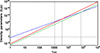 |
Fig. 1. ΛωsCDM density parameters: Λ (dotted gray), pressureless matter (dashed blue), radiation (solid red), and matter with pressure (dotted-dashed green); vertical black lines (from left to right) mark the following redshifts: recombination, pressureless matter–radiation equivalence, and pressureless matter–matter with pressure equivalence. |
Comparison between a barotropic fluid with constant ωs > 0 and EDE paradigms.
3. Experimental setup
To prove the existence of our additional fluid with density, Ωs(1 + z)3(1 + ωs), we define the underlying background cosmology as an extension of the standard ΛCDM framework, in which the comoving distance is defined as
 (10)
(10)
where the parameters describing the expansion history enter in the definition of the Hubble parameter:
![Mathematical equation: $$ \begin{aligned} H(z) = H_0 \left[\Omega _\nu (z)+{\sum }_i \Omega _i (1+z)^{3(1+\omega _i)}\right]^{1/2}; \end{aligned} $$](/articles/aa/full_html/2026/03/aa56049-25/aa56049-25-eq11.gif) (11)
(11)
here, the set, i = {Λ, m, γ, s}, labels the cosmological constant, dust, radiation, and matter with pressure, respectively, exhibiting barotropic indexes as ωi = { − 1, 0, 1/3, ωs}. The energy density of neutrinos Ων(z) scales as radiation (with EoS ων = 1/3) at early times and as matter (with ων = 0) at late times. Ensuring a spatially flat Universe, Ωk = 0, naturally implies ΩΛ = 1 − Ωm − Ωs − Ωγ − Ων. Thus, from Eq. (10) we can define the luminosity distance DL(z) = (1 + z)DM(z) and the diameter angular distance DA(z) = DM(z)/(1 + z).
3.1. Numerical results
We utilized the following datasets: the Pantheon+ sample of SNe Ia, the second data release (DR2) of baryonic acoustic oscillations (BAO) from the Dark Energy Spectroscopic Instrument (DESI), hereafter dubbed DR2 DESI-BAO, and the CMB data, indicated in detail below and in Appendix A.
3.1.1. Pantheon+ and SH0ES.
The Pantheon+ is a catalog of 1701 SNe Ia with redshifts of z ∈ [0, 2.3]. It comprises 18 different samples (Scolnic et al. 2022) and includes the released SH0ES Cepheid host distance anchors that provide the value of H0 that is in tension with CMB determination (Brout et al. 2022).
When using SH0ES Cepheid host distances, the 1701 SN distance modulus residuals are given by
 (12)
(12)
in which μi are the inferred SN distance moduli and μC, i are the Cepheid-calibrated host-galaxy distance moduli by SH0ES; the model’s distance moduli are
 (13)
(13)
where mi are the rest-frame B-band apparent magnitudes of each SN Ia, and the rest-frame B-band absolute magnitude, M, can be viewed as a nuisance parameter and marginalized (Conley et al. 2011). Thus, the cosmological parameters can be constrained by maximizing the log-likelihood
 (14)
(14)
where C = CSN + CC is the total covariance matrix of SNe and Cepheid host distances (accounting for both statistical and systematic errors)7.
3.1.2. DR2 DESI-BAO.
The DR2 DESI-BAO dataset is shown in Table A.1. We utilized a total of ND = 13 measurements: six transverse distances, DM; six Hubble rate distances, DH (six data points); and one angle-averaged distance, DV, all normalized over comoving sound horizon at the baryon drag redshift, zd, i.e., rd = rs(zd) (Abdul Karim et al. 2025). Breaking the rd − H0 degeneracy is mandatory to provide the explicit expression of rd as a function of the model parameters given in Sect. 2. Here, we only fixed zd = 1059.94 ± 0.30 (Planck Collaboration VI 2020). Provided that DM is given in Eq. (10), the other two distance measurements are given by
 (15)
(15)
Thus, the total BAO log-likelihood is given by
![Mathematical equation: $$ \begin{aligned} \ln \mathcal{L} _{\rm BAO} \propto -\frac{1}{2} \sum _{i = 1}^{N_{D}}\!\left[Y_{i}-Y(z_{i})\right]^{T}\!C_{\rm BAO}^{-1}\!\left[Y_{i}-Y(z_{i})\right], \end{aligned} $$](/articles/aa/full_html/2026/03/aa56049-25/aa56049-25-eq16.gif) (16)
(16)
with Yi denoting the DR2 measurements and Y(zi) = {DM(zi)/rd, DH(zi)/rd, DV(zi)/rd} given in Eqs. (10) and (15). Here, CBAO indicates the BAO covariance matrix8.
3.1.3. CMB data.
We adopted the Planck 2018 CMB high-ℓ TTTEEE, low-ℓ TTEE, and lensing likelihoods. In particular, we used the Plik (Planck Collaboration V 2020) high-ℓ likelihood for TT over 30 ≤ ℓ ≤ 2508 and for TE and EE over 30 ≤ ℓ ≤ 1996. The low-ℓ TT and EE likelihoods cover 2 ≤ ℓ ≤ 29 and are based on the Commander algorithm and SimAll likelihood, respectively (Aghanim et al. 2020; Planck Collaboration IV 2020). The CMB Plik lensing likelihood is included following Planck Collaboration VIII (2020).
By accounting for all the above described datasets, we can deduce the model cosmological parameters by maximizing the total log-likelihood function defined as
 (17)
(17)
using the priors given by Table 2.
Priors on the model cosmological parameters.
MCMC fitting was performed using our modified version of CLASS9. This code solves the Boltzmann equations for perturbations in the early Universe and accounts for the following components: photons, baryons, cold dark matter, neutrinos, dark energy (in the form of a cosmological constant Λ), and our extra matter fluid with pressure10. Specifically, in agreement with the Planck analysis, we assumed two massless neutrino species and one massive species with mν = 0.06 eV, leading to Neff = 3.046 (Ade et al. 2019). In our analysis, chain convergence is assumed to be achieved when the Gelman–Rubin statistic satisfies R − 1 < 0.02 (Gelman & Rubin 1992).
The results are summarized in Table 3. The ΛωsCDM model yields a better fit to the data, with  , compared to χΛ2 = 4115.48 for the ΛCDM model; this corresponds to
  . Then, to estimate the statistical preference, we computed the Bayesian evidence using the public code MCEvidence (Heavens et al. 2017)11. A model comparison was done by computing Δlog B = log Bs − log BΛ = +6.2, which yields decisive evidence in favor of the ΛωsCDM scenario based on the modified Jeffreys’ scale (Trotta 2008).
MCMC results for ΛωsCDM and ΛCDM models.
Using the results of the ΛωsCDM model from Table 3, we were able to compute the equivalence epochs among fluids. Figure 1 displays the density parameters, Ωi(z) = Ωi(1 + z)3(1 + ωi), of all fluids12. In particular, we mark the following epochs with vertical black lines (from left to right): (i) the recombination redshift, z★ = 1089.92; (ii) the equivalence redshift between the pressureless matter and radiation (photons and neutrinos) equivalence redshift (zeq ≈ 3600); and (iii) the equivalence redshift between matter with and without pressure (zms ≈ 68400). From the plot it also evident that our matter fluid with pressure is (a) subdominant with respect to pressureless matter and radiation (photons and neutrinos) at z★, and (b) subdominant with respect to photons at late times and photons+neutrinos at early times. For the above reasons, all the other model parameters were not significantly modified –with respect to the ΛCDM case– by the presence of such a further contribution. The corresponding contour plots, obtained using GetDist, are portrayed in Fig. B.1.
3.2. Physical consequences
In our picture, forcing a positive EoS and a fluid in the Zel’dovic limit implies a result of
 (18)
(18)
with  . This kind of fluid, with an EoS similar to radiation and here reinterpreted as matter with pressure, can mainly be attributed to specific cases of interest.
3.2.1. Unlikely physical scenarios
Below, we report two direct possibilities that appear to be unlikely.
3.2.1.1. Non-gauge fields such as the Proca Lagrangian.
In such a case, the Hubble tension can be solved including the presence of massive electromagnetic fields, where the action of photon mass, mP, reduces the EoS. For example, (a) ensuring the spatial component of the vector potential, A, and the magnetic field, B, vanish, say A = B = 0, and (b) that for the scalar potential, A0, and the electric field, E, the relation mP2A02 ≪ E2 holds, we end up with
 (19)
(19)
In a thermal background at temperature T, we have the following scalings: A0 ≈ T and E2 ≈ 2T4. Thus, using the above value of ϵ and the temperature at recombination T★ = 0.26 eV, we obtain  eV, which is, however, excluded by the most conservative existing upper limit on the photon mass mγ < 10−18 eV obtained from the solar-wind magnetic-field structure (Ryutov 2007).
3.2.1.2. Dark photons.
Highly debated and recently put under examination, dark photons are hypothetical massive gauge bosons associated with a dark-sector hidden U(1)D symmetry. They may have a small kinetic mixing with massless photons and very weak or no direct coupling to standard model matter (Cline 2024). Massive dark photons behave as Proca fields:
 (20)
(20)
but with much greater freedom, since dark photons are not subject to the same tight experimental bounds as standard photons. Therefore, for these constituents, we simply took the previous bound,  eV.
eV.
3.2.2. Most plausible physical interpretation: A thermal, semi-relativistic scalar component
In view of the above, our matter with pressure fluid may be interpreted either as a thermalized scalar field, whose nature can be associated with the quasi-quintessence, or as vector fields, in which the Proca field could represent an immediate and plausible explanation. We did not investigate alternatives making use of extended theories of gravity and/or modifications as they are being beyond the scope of this work (see, e.g., van der Westhuizen et al. 2025 and Paliathanasis 2025a,b).
The MCMC constraints indicate that the additional component behaves as a quasi-radiation fluid, with a constant ϵ > 0 and a small but non-vanishing energy density, which remains subdominant with respect to the standard radiation sector at recombination, roughly reading Ωs/Ωγ ∼ 1/3. In this regime, the fluid is naturally interpreted as an effectively relativistic species, whose pressure is mildly reduced by a finite mass scale.
Among the various possibilities discussed above, a thermal, semi-relativistic scalar component may be the most likely counterpart to associate with our fluid. In this case, the desired EoS is obtained in a standard kinetic-theory approximation. The simplest approach is to consider, for example, an additional purely relativistic species assumed to be a sterile neutrino. Sterile neutrinos imply severe bounds on the effective number of relativistic species, whereas scalar fields come as an extension of the generalized K essence described in Appendix C.
In the semi-relativistic approximation, we have
 (21)
(21)
where mS is the mass and κ ≈ 2.7 for neutrinos (from Fermi-Dirac statistic) and κ ≈ 3.2 for scalars (from Bose-Einstein statistic). Both massive components behave as radiation with ωS ≈ 1/3 when mS ≪ T and as pressureless matter with ωS ≈ 0 when mS ≫ T. Limits on the mass, for example at the recombination, can be obtained as follows:
 (22)
(22)
From the above discussion, it immediately appears evident that sterile neutrinos, or Majorana fermions more broadly, shall be accounted for in Neff; moreover, since in our MCMC fits it is fixed to the standard value of Neff = 3.046, any mass estimates would be physically incorrect. In addition, recent developments seem to indicate that sterile neutrinos appear quite disfavored, as they have not been detected by independent experiments so far (see, e.g., Grimm et al. 2025).
Conversely, for thermal scalar fields (namely bosons) there is no such limitation. We thus obtain
 (23)
(23)
This interpretation has two attractive features, which are summarized below.
-
It naturally explains why the extra component is very close to radiation. Indeed, the fluid is simply a thermal species that is still semi-relativistic at z★. Accordingly, it contributes to early-time expansion, and precisely to the sound horizon integral, without requiring EDE; but it is also constantly subdominant throughout the evolution of the Universe.
-
It clarifies why the component does not behave as an additional clustering agent at late times. For a barotropic fluid with constant ωs and adiabatic perturbations, the rest-frame sound speed is cs, s2 = ωs; hence, pressure support prevents gravitational growth once modes enter the horizon, in close analogy with the photon sector. We faced this point later while dealing with Newtonian perturbations.
A more accurate study that could exclude dark photons and exotic species could be pursued in future developments. We would check whether, statistically speaking, our fluid may be favored to exist even at late times.
3.3. Comparison with Big Bang nucleosynthesis constraints
The existence of a new barotropic fluid not only alters the expansion rate of the Universe at any epoch, but could also affect the primordial abundances of light elements produced during Big Bang nucleosynthesis (BBN). In this work, we investigated the consistency with the observed 4He mass fraction value Yp = 0.2450 ± 0.0050 (with statistical and systematic errors) and the CMB-inferred ratio between the number densities of photons and baryons η = (6.104 ± 0.058)×10−10 (Navas et al. 2024). We use simplified analytical calculations, excluding the possible identification of the extra fluid with an additional neutrino species as stated above, and we verified the consistency with the standard BBN framework when Ωs = 0.
At temperatures of T ≫ 1 MeV, proton and neutron number densities are the same because the weak interaction rate Γ(T) = qT5, with q = 9.6 × 10⁻²² MeV−4 (Matei et al. 2025), is much larger than the expansion rate:
![Mathematical equation: $$ \begin{aligned} H(T) = \frac{T^2}{M_p} \left[\frac{8\pi ^3g(T)}{90}\right]^{1/2}\left[1+\delta _s(T)\right]^{1/2}\,, \end{aligned} $$](/articles/aa/full_html/2026/03/aa56049-25/aa56049-25-eq53.gif) (24)
(24)
where g(T) is the number of relativistic degrees of freedom, which depends on the primordial plasma temperature, and
![Mathematical equation: $$ \begin{aligned} \delta _s(T) = \frac{\Omega _s}{\Omega _r} \left[\frac{g_S(T)}{g_S(T_0)}\right]^{\omega _s-1/3} \left(\frac{T}{T_0}\right)^{3 \omega _s-1}\,. \end{aligned} $$](/articles/aa/full_html/2026/03/aa56049-25/aa56049-25-eq54.gif) (25)
(25)
The ratio between the entropy degrees of freedom, gS, computed at T, and the CMB temperature, T0, appears as a consequence of the entropy conservation, gS(T)T3a3 = const, because from MCMC fits we have the current extra-fluid density parameter at T0, but in Eq. (24) it has to be evaluated at T. In fact, the temperature of the plasma is not an exact proxy of the scale factor, a = (1 + z)−1, which is altered by changes in the number of relativistic species across the evolution of the Universe.
As the Universe cools down, the above competing rates become comparable –Γ(Tf) = H(Tf)– at the “freeze-out” temperature –Tf ≃ 0.8 MeV– for which protons and neutrons are locked in a ratio of 5 : 1. This is the onset of the BBN.
The first nuclear reaction involves the synthesis of deuterium nuclei. However, because of the extremely high abundances of high-energy photons, compared to baryons, deuterium and 4He syntheses are delayed until the plasma temperature drops well below the binding energy of a deuterium nucleus, BD = 2.224 MeV. This is referred as to as the deuterium bottleneck. Thus, the production of deuterium nuclei starts when their creation and destruction rates become equal. This occurs at a temperature of Td ≃ 0.06 MeV, which can be evaluated as
![Mathematical equation: $$ \begin{aligned} T_{\rm d} \simeq - B_D\left\{ \ln \eta + \frac{3}{2} \ln \left(\frac{4 \pi T_{\rm d}}{m_{\rm n}}\right) + \ln \left[\frac{3 \zeta (3)}{\pi ^2}\right]\right\} ^{-1} \end{aligned} $$](/articles/aa/full_html/2026/03/aa56049-25/aa56049-25-eq55.gif) (26)
(26)
(Mukhanov 2005), where mn is the neutron mass. Thus, the mass fraction of 4He can be evaluated using the neutron-to-proton number density ratio (n/p)d evaluated across freeze-out and deuterium production phases; i.e.,
 (27)
(27)
where Δm = 1.293 MeV is the neutron–proton mass difference and τn ≈ 880 s is the neutron mean lifetime. The cosmic times at freeze-out and deuterium production, tf and td, respectively, were computed from the relation t(Tx) = ∫Tx+∞dT/[T H(T)]. Moreover, in evaluating the cosmic times and δs(T), one has to take into account that at T < Tf neutrinos decouple from the other particles, while keeping the same temperature; afterwards, at T ≲ me, the e± pairs (with masses of me) in the thermal background begin to annihilate, heating up the photon background relatively to the decoupled neutrinos. Here, we considered the e± annihilation to be completely settled below an effective temperature of Te ≃ 0.15 MeV. In view of these considerations, our calculations consider
The results are shown in Fig. 2, where in the standard BBN we recovered Yp = 0.2463, whereas in our scenario we obtained the value Yp = 0.02478 ± 0.0021, which is fully consistent with the observational bounds.
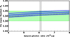 |
Fig. 2. BBN constraints in η–Yp plane for the ΛωsCDM model (blue curve with the light blue 1σ error bands), compared with the standard result (dashed black curve) and the observational constraints on Yp (green box) and η (gray box). |
3.4. Linear perturbations
Our extra component was modeled as a barotropic perfect fluid with a constant and positive EoS, Ps = ωsρs, with an index ωs –according to our fits– close to, but slightly below, the photon value ωγ = 1/3. Accordingly, the new species behaves as a “quasi-radiation” component: it contributes to the early-time background expansion and to the primordial plasma properties, while remaining subdominant with respect to the standard radiation sector.
It is important to clarify what we mean by “no clustering”. This does not imply the absence of perturbations. Rather, it means that, once a Fourier mode enters the horizon, the density contrast of the ωs–fluid does not develop a gravitationally growing mode that could seed, or substantially contribute to, late-time structure formation. This behavior is analogous to radiation; i.e., photon perturbations exist and are observable (e.g., through acoustic physics), but they do not collapse into bound structures.
For a barotropic fluid with constant ωs and adiabatic perturbations (no intrinsic entropy mode), the rest-frame sound speed equals the adiabatic one,
 (28)
(28)
so, for ωs = 𝒪(10−1), the pressure support is relativistically large. On subhorizon scales, the competition between pressure support and gravity leads to a damped acoustic behavior for δs ≡ δρs/ρs, with an effective frequency ∼cs, sk/a. This is conveniently summarized by the Jeans scale estimate,
 (29)
(29)
which enters the density-contrast equation,
 (30)
(30)
which was written in a Newtonian context; i.e., analogous to the more complicated fully relativistic version.
Our findings show that, using Eq. (28), the Jeans length is on order the Hubble radius. Hence, for subhorizon modes (k ≫ aH) we have
 (31)
(31)
and δs undergoes acoustic oscillations with Hubble damping rather than a growing gravitational instability. Consequently, our new fluid does not act as an additional clustering component at current times. Its crucial contribution lies in the early-time expansion and horizon-scale dynamics, consistently with our Boltzmann treatment of perturbations.
Future works will explore the fully relativistic versions of Eq. (30). However, the main outcome cannot depart from the one above reported, indicating that the ΛωsCDM paradigm does not depart significantly from the expectations of the standard cosmological model.
4. Final remarks
In this work, we focused on the early-time Universe to heal the observational H0 tension and proposed an alternative view to EDE models, namely invoking the existence of an additional barotropic fluid component that is physically inspired by stiff matter-like fluids exhibiting relativistic properties differently from dust. In so doing, we ensured this fluid obeyed the Zel’dovic condition on the EoS; i.e., it had to possess ωs > 0. This matter-like constituent was constructed with nonnegligible pressure, which is quite distinct from both radiation and standard EDE candidates, as well as pure dust-like counterparts or neutrinos. Thus, by introducing such a component into the early cosmological dynamics, we directly altered the expansion rate, H(z), and the comoving sound horizon, rs, prior to recombination, modifying, moreover, the sound speed, cs. This enabled an effective increase in H0 through a minimal and direct extension of the ΛCDM paradigm, which we call the ΛωsCDM model. To prevent any significant modification of cosmic measurements, we required the additional barotropic component to remain subdominant with respect to radiation, matter, and dark energy throughout the entire cosmic-expansion history. Thus, we carried out a full cosmological parameter estimation using a MCMC simulation, involving Pantheon+ with SH0ES SNe, DR2 DESI-BAO, and the Planck 2018 CMB high-ℓ TTTEEE, low-ℓ TTEE and lensing likelihoods. To this end, we modified the CLASS code (Lesgourgues 2011) to include the dynamics of the extra fluid and performed the analysis in accordance with the latest Planck observational constraints. In this respect, we included radiation and neutrino contributions, employing the assumption of spatial flatness.
We showed that the proposed extension is favored with respect to the ΛCDM benchmark model, while our findings ruled out the case of a purely stiff fluid with EoS ω = 1, instead favoring a scenario in which the fluid exhibits an EoS slightly below that of photons, ωs ≲ ωγ, and a density parameter smaller than the photons’ background, which is Ωs/Ωγ ≃ 0.33. Indeed, we demonstrated that the additional fluid contribution remained significantly smaller than that of radiation and thus did not produce any substantial alteration in the CMB anisotropy power spectrum.
Afterwards, we discussed the physical implications of such a fluid, emphasizing its phenomenological consistency and theoretical plausibility. We thus propose that the fluid may be interpreted in view of a possible Proca-like field, where the effect of nonzero mass for the vector field can alter the EoS, departing from the genuine case given by radiation. We thus conclude that at least two vector fields may be present just before the last scattering surface, without, however, excluding more exotic scenarios involving dark radiation, axions, and so on. Based on these considerations, we evaluated the 4He mass fraction, Yp, produced during the BBN with the inclusion of our extra fluid, and we verified the consistency with the observational bounds.
After this crucial point, we explored the linear Newtonian perturbations, showing analogy between our new fluid and pure radiation. Accordingly, we conclude that it is unlikely that our new fluid would influence the clustering without significantly altering observations at current times.
We also inferred constraints on equivalence and transition between epochs between pressureless matter and radiation (occurring at zeq ≈ 3600) and between matter with and without pressure (occurring at zms ≈ 68400). The matter fluid with pressure is subdominant with respect to pressureless matter and radiation at z★, and always subdominant with respect to radiation. These features show that all other constituents are not significantly modified by the presence of this kind of further contribution.
Future works will compare this matter with pressure fluid through other approaches that predict matter with pressure, by complicating the barotropic factors, or simply involving thermodynamic alternatives other than a constant and positive ωs. Moreover, we will see the influence on structure formation of this fluid and, above all, its fundamental nature in more detail; thus, we will further explore the role of Proca-like fields in early-time cosmology. A direct comparison with additional constituents, such as neutrinos, relativistic matter, and so on. will also be the object of future speculations. Last but not least, further experimental analyses will be pursued with the aim of refining our bounds, taking a deeper look at perturbations, and adopting a fully relativistic first- and second-order analysis.
Acknowledgments
YC acknowledges Francesco Pace for valuable discussions and is grateful to Vivian Poulin for support during his stay at LUPM, where this work was finalized. OL acknowledges Maryam Azizinia for discussion and support by the Fondazione ICSC, Spoke 3 Astrophysics and Cosmos Observations National Recovery and Resilience Plan (Piano Nazionale di Ripresa e Resilienza, PNRR) Project ID CN00000013 “Italian Research Center on High-Performance Computing, Big Data and Quantum Computing” funded by MUR Missione 4 Componente 2 Investimento 1.4: Potenziamento strutture di ricerca e creazione di “campioni nazionali di R&S (M4C2-19 )” – Next Generation EU (NGEU).
References
- Abdul Karim, M., Aguilar, J., Ahlen, S., et al. 2025, Phys. Rev. D, 112, 083515 [Google Scholar]
- Ade, P., Aguirre, J., Ahmed, Z., et al. 2019, JCAP, 2019, 056 [Google Scholar]
- Aghanim, N., Akrami, Y., Ashdown, M., et al. 2020, A&A, 641, A6 [NASA ADS] [CrossRef] [EDP Sciences] [Google Scholar]
- Alfano, A. C., Luongo, O., & Muccino, M. 2025, JHEAp, 46, 100348 [Google Scholar]
- Anton, H., & Schmidt, P. C. 1997, Intermetallics, 5, 449 [Google Scholar]
- Aviles, A., Gruber, C., Luongo, O., & Quevedo, H. 2012, Phys. Rev. D, 86, 123516 [CrossRef] [Google Scholar]
- Bamba, K., Capozziello, S., Nojiri, S., & Odintsov, S. D. 2012, Astrophys. Space Sci., 342, 155 [NASA ADS] [CrossRef] [Google Scholar]
- Banik, I., & Kalaitzidis, V. 2025, MNRAS, 540, 545 [Google Scholar]
- Belfiglio, A., Giambò, R., & Luongo, O. 2023, Class. Quant. Grav., 40, 105004 [NASA ADS] [CrossRef] [Google Scholar]
- Belfiglio, A., Carloni, Y., & Luongo, O. 2024, Phys. Dark Univ., 44, 101458 [Google Scholar]
- Bertone, G., & Tait, M. P. T. 2018, Nature, 562, 51 [Google Scholar]
- Blinov, N., Keith, C., & Hooper, D. 2020, JCAP, 06, 005 [Google Scholar]
- Boshkayev, K., D’Agostino, R., & Luongo, O. 2019, Eur. Phys. J. C, 79, 332 [NASA ADS] [CrossRef] [Google Scholar]
- Boshkayev, K., Konysbayev, T., Kurmanov, E., Luongo, O., & Muccino, M. 2020, Galaxies, 8, 74 [Google Scholar]
- Boshkayev, K., Konysbayev, T., Luongo, O., Muccino, M., & Pace, F. 2021, Phys. Rev. D, 104, 023520 [Google Scholar]
- Braglia, M., Emond, W. T., Finelli, F., Gumrukcuoglu, A. E., & Koyama, K. 2020, Phys. Rev. D, 102, 083513 [Google Scholar]
- Brout, D., Scolnic, D., Popovic, B., et al. 2022, ApJ, 938, 110 [NASA ADS] [CrossRef] [Google Scholar]
- Capozziello, S., D’Agostino, R., & Luongo, O. 2018, Phys. Dark Univ., 20, 1 [Google Scholar]
- Capozziello, S., D’Agostino, R., Giambò, R., & Luongo, O. 2019a, Phys. Rev. D, 99, 023532 [Google Scholar]
- Capozziello, S., D’Agostino, R., & Luongo, O. 2019b, Int. J. Mod. Phys. D, 28, 1930016 [NASA ADS] [CrossRef] [Google Scholar]
- Capozziello, S., D’Agostino, R., Lapponi, A., & Luongo, O. 2023, Eur. Phys. J. C, 83, 175 [Google Scholar]
- Carloni, Y., & Luongo, O. 2025, Class. Quant. Grav., 42, 075014 [Google Scholar]
- Carloni, Y., Luongo, O., & Muccino, M. 2025, Phys. Rev. D, 111, 023512 [Google Scholar]
- Chatrchyan, A., Niedermann, F., Poulin, V., & Sloth, M. S. 2025, Phys. Rev. D, 111, 043536 [Google Scholar]
- Chavanis, P.-H. 2015a, Phys. Rev. D, 92, 103004 [Google Scholar]
- Chavanis, P.-H. 2015b, Eur. Phys. J. Plus, 130, 130 [Google Scholar]
- Chavanis, P.-H. 2016, Phys. Lett. B, 758, 59 [Google Scholar]
- Chiba, T. 2006, Phys. Rev. D, 73, 063501 [Google Scholar]
- Cline, J. M. 2024, in 58th Rencontres de Moriond on Electroweak Interactions and Unified Theories [Google Scholar]
- Conley, A., Guy, J., Sullivan, M., et al. 2011, ApJS, 192, 1 [Google Scholar]
- Cortês, M., & Liddle, A. R. 2024, MNRAS, 531, L52 [Google Scholar]
- D’Agostino, R., Luongo, O., & Muccino, M. 2022, Class. Quantum Gravity, 39, 195014 [Google Scholar]
- Dainotti, M. G., De Simone, B., Schiavone, T., et al. 2021, ApJ, 912, 150 [NASA ADS] [CrossRef] [Google Scholar]
- Dainotti, M. G., De Simone, B., Schiavone, T., et al. 2022, Galaxies, 10, 24 [NASA ADS] [CrossRef] [Google Scholar]
- Dainotti, M. G., De Simone, B., Garg, A., et al. 2025, JHEAp, 48, 100405 [Google Scholar]
- De Simone, B., van Putten, M. H. P. M., Dainotti, M. G., & Lambiase, G. 2025, JHEAp, 45, 290 [Google Scholar]
- Desjacques, V., Chluba, J., Silk, J., de Bernardis, F., & Doré, O. 2015, MNRAS, 451, 4460 [Google Scholar]
- Doran, M., & Robbers, G. 2006, JCAP, 06, 026 [Google Scholar]
- Doran, M., & Wetterich, C. 2003, Nucl. Phys. B Proc. Suppl., 124, 57 [Google Scholar]
- Doran, M., Schwindt, J.-M., & Wetterich, C. 2001, Phys. Rev. D, 64, 123520 [Google Scholar]
- Dunsby, P. K. S., & Luongo, O. 2016, Int. J. Geom. Meth. Mod. Phys., 13, 1630002 [NASA ADS] [CrossRef] [Google Scholar]
- Dunsby, P. K. S., Luongo, O., & Reverberi, L. 2016, Phys. Rev. D, 94, 083525 [Google Scholar]
- Dunsby, P. K. S., Luongo, O., & Muccino, M. 2024a, Phys. Rev. D, 109, 023510 [Google Scholar]
- Dunsby, P. K. S., Luongo, O., Muccino, M., & Pillay, V. 2024b, Phys. Dark Univ., 46, 101563 [Google Scholar]
- Dymnikova, I., & Khlopov, M. 1998, Grav. Cosmol. Suppl., 4, 50 [Google Scholar]
- Dymnikova, I., & Khlopov, M. 2000, Mod. Phys. Lett. A, 15, 2305 [Google Scholar]
- Dymnikova, I., & Khlopov, M. 2001, Eur. Phys. J. C, 20, 139 [Google Scholar]
- Evslin, J., Sen, A. A., & Ruchika, 2018, Phys. Rev. D, 97, 103511 [Google Scholar]
- Faber, T., & Visser, M. 2006, MNRAS, 372, 136 [Google Scholar]
- Fabris, J. C., Velten, H. E. S., Ogouyandjou, C., & Tossa, J. 2011, Phys. Lett. B, 694, 289 [Google Scholar]
- Gelman, A., & Rubin, D. 1992, Stat. Sci., 7, 457 [NASA ADS] [Google Scholar]
- Gomez-Valent, A., & Solà Peracaula, J. 2024, ApJ, 975, 64 [Google Scholar]
- Gómez-Valent, A., Zheng, Z., Amendola, L., Pettorino, V., & Wetterich, C. 2021, Phys. Rev. D, 104, 083536 [Google Scholar]
- Grimm, N., Bonvin, C., & Tutusaus, I. 2025, Nature Commun., 16, 9399 [Google Scholar]
- Grøn, O. G. 2024, Axioms, 13, 526 [Google Scholar]
- Grossi, M., & Springel, V. 2009, MNRAS, 394, 1559 [Google Scholar]
- Heavens, A., Fantaye, Y., Mootoovaloo, A., et al. 2017, ArXiv e-prints [arXiv:1704.03472] [Google Scholar]
- Hu, W., & Dodelson, S. 2002, ARA&A, 40, 171 [Google Scholar]
- Hu, J.-P., & Wang, F.-Y. 2023, Universe, 9, 94 [CrossRef] [Google Scholar]
- Hu, J. P., Jia, X. D., Hu, J., & Wang, F. Y. 2024, ApJ, 975, L36 [Google Scholar]
- Kamionkowski, M., & Riess, A. G. 2023, Ann. Rev. Nucl. Part. Sci., 73, 153 [NASA ADS] [CrossRef] [Google Scholar]
- Kou, R., & Lewis, A. 2025, JCAP, 01, 033 [Google Scholar]
- Lee, N., Braglia, M., & Ali-Haïmoud, Y. 2025, ArXiv e-prints [arXiv:2504.07966] [Google Scholar]
- Lesgourgues, J. 2011, ArXiv e-prints [arXiv:1104.2932] [Google Scholar]
- Linder, E. V., & Robbers, G. 2008, JCAP, 06, 004 [Google Scholar]
- Linder, E. V., & Scherrer, R. J. 2009, Phys. Rev. D, 80, 023008 [Google Scholar]
- Luongo, O. 2025, Class. Quant. Grav., 42, 225005 [Google Scholar]
- Luongo, O., & Muccino, M. 2018, Phys. Rev. D, 98, 103520 [CrossRef] [Google Scholar]
- Luongo, O., & Muccino, M. 2020, A&A, 641, A174 [NASA ADS] [CrossRef] [EDP Sciences] [Google Scholar]
- Luongo, O., & Muccino, M. 2022, in 15th Marcel Grossmann Meeting on Recent Developments in Theoretical and Experimental General Relativity, Astrophysics, and Relativistic Field Theories [Google Scholar]
- Luongo, O., & Muccino, M. 2024, A&A, 690, A40 [NASA ADS] [CrossRef] [EDP Sciences] [Google Scholar]
- Luongo, O., & Quevedo, H. 2014, Gen. Rel. Grav., 46, 1649 [NASA ADS] [CrossRef] [Google Scholar]
- Lynch, G. P., Knox, L., & Chluba, J. 2024a, Phys. Rev. D, 110, 083538 [Google Scholar]
- Lynch, G. P., Knox, L., & Chluba, J. 2024b, Phys. Rev. D, 110, 063518 [Google Scholar]
- Maggiore, M., Hollenstein, L., Jaccard, M., & Mitsou, E. 2011, Phys. Lett. B, 704, 102 [Google Scholar]
- Matei, T. M., Croitoru, C. A., & Harko, T. 2025, Eur. Phys. J. C, 85, 1092 [Google Scholar]
- Mirpoorian, S. H., Jedamzik, K., & Pogosian, L. 2025, Phys. Rev. D, 111, 083519 [Google Scholar]
- Mukhanov, V. 2005, Physical Foundations of Cosmology (Oxford: Cambridge University Press) [Google Scholar]
- Mukhopadhyay, U., Ghosh, P. P., Khlopov, M., & Ray, S. 2011, Int. J. Theor. Phys., 50, 939 [Google Scholar]
- Navas, S., Amsler, C., Gutsche, T., et al. 2024, Phys. Rev. D, 110, 030001 [CrossRef] [Google Scholar]
- Niedermann, F., & Sloth, M. S. 2020, Phys. Rev. D, 102, 063527 [NASA ADS] [CrossRef] [Google Scholar]
- Niedermann, F., & Sloth, M. S. 2021, Phys. Rev. D, 103, L041303 [Google Scholar]
- Nygaard, A., Holm, E. B., Tram, T., & Hannestad, S. 2023, ArXiv e-prints [arXiv:2307.00418] [Google Scholar]
- Odintsov, S. D., Sáez-Chillón Gómez, D., & Sharov, G. S. 2021, Nucl. Phys. B, 966, 115377 [Google Scholar]
- Paliathanasis, A. 2025a, JCAP, 09, 067 [Google Scholar]
- Paliathanasis, A. 2025b, Phys. Dark Univ., 49, 101993 [Google Scholar]
- Pan, S., Yang, W., & Paliathanasis, A. 2020, MNRAS, 493, 3114 [Google Scholar]
- Pedrotti, D., Jiang, J.-Q., Escamilla, L. A., da Costa, S. S., & Vagnozzi, S. 2025, Phys. Rev. D, 111, 023506 [Google Scholar]
- Pettorino, V., Amendola, L., & Wetterich, C. 2013, Phys. Rev. D, 87, 083009 [Google Scholar]
- Planck Collaboration IV. 2020, A&A, 641, A4 [NASA ADS] [CrossRef] [EDP Sciences] [Google Scholar]
- Planck Collaboration V. 2020, A&A, 641, A5 [NASA ADS] [CrossRef] [EDP Sciences] [Google Scholar]
- Planck Collaboration VI. 2020, A&A, 641, A6 [NASA ADS] [CrossRef] [EDP Sciences] [Google Scholar]
- Planck Collaboration VIII. 2020, A&A, 641, A8 [NASA ADS] [CrossRef] [EDP Sciences] [Google Scholar]
- Poulin, V., Smith, T. L., Karwal, T., & Kamionkowski, M. 2019, Phys. Rev. Lett., 122, 221301 [Google Scholar]
- Poulin, V., Smith, T. L., & Karwal, T. 2023, Phys. Dark Univ., 42, 101348 [Google Scholar]
- Riess, A. G., Yuan, W., Macri, L. M., et al. 2022, ApJ, 934, L7 [NASA ADS] [CrossRef] [Google Scholar]
- Ryutov, D. D. 2007, Plasma Phys. Control. Fusion, 49, B429 [Google Scholar]
- Sabla, V. I., & Caldwell, R. R. 2022, Phys. Rev. D, 106, 063526 [Google Scholar]
- Scherrer, R. J., & Sen, A. A. 2008a, Phys. Rev. D, 78, 067303 [Google Scholar]
- Scherrer, R. J., & Sen, A. A. 2008b, Phys. Rev. D, 77, 083515 [Google Scholar]
- Schöneberg, N., Franco Abellán, G., Pérez Sánchez, A., et al. 2022, Phys. Rept., 984, 1 [CrossRef] [Google Scholar]
- Scolnic, D., Brout, D., Carr, A., et al. 2022, ApJ, 938, 113 [NASA ADS] [CrossRef] [Google Scholar]
- Shahalam, M., Pathak, S. D., Verma, M. M., Khlopov, M. Y., & Myrzakulov, R. 2015, Eur. Phys. J. C, 75, 395 [Google Scholar]
- Smith, T. L., Poulin, V., Bernal, J. L., et al. 2021, Phys. Rev. D, 103, 123542 [Google Scholar]
- Steinhardt, P. J., Wang, L.-M., & Zlatev, I. 1999, Phys. Rev. D, 59, 123504 [Google Scholar]
- Trotta, R. 2008, Contemp. Phys., 49, 71 [Google Scholar]
- Vagnozzi, S. 2023, Universe, 9, 393 [NASA ADS] [CrossRef] [Google Scholar]
- van der Westhuizen, M., Figueruelo, D., Thubisi, R., et al. 2025, Phys. Dark Univ., 50, 102107 [Google Scholar]
- Wetterich, C. 2004, Phys. Lett. B, 594, 17 [NASA ADS] [Google Scholar]
- Wolf, W. J., & Ferreira, P. G. 2023, Phys. Rev. D, 108, 103519 [NASA ADS] [CrossRef] [Google Scholar]
- Yang, W., Pan, S., Paliathanasis, A., Ghosh, S., & Wu, Y. 2019, MNRAS, 490, 2071 [Google Scholar]
Strong criticisms to these outcomes can be found in Carloni et al. (2025), Luongo & Muccino (2024), and Alfano et al. (2025).
Current bounds show that ultralight or supermassive fields could be suitable candidates, excluding de facto WIMPs (Bertone & Tait 2018). Alternatives may be extensions of Einstein’s gravity (Capozziello et al. 2019b) or space-time solutions, within general relativity, behaving as particles (Luongo 2025).
Given that this discrepancy is corroborated by multiple independent probes, it is unlikely that a single systematic error accounts for the full disagreement, as stated above.
In this work, the redshifts of recombination, photon decoupling, and last scattering are interchangeable, following the convention used in Hu & Dodelson (2002), Desjacques et al. (2015), Aghanim et al. (2020), Kamionkowski & Riess (2023), Lynch et al. (2024b), Mirpoorian et al. (2025), and Kou & Lewis (2025).
For the intriguing case of dark matter (instead of pure matter) with pressure, we refer the reader to Faber & Visser (2006), Dunsby et al. (2016), Luongo & Muccino (2022), Dunsby et al. (2024a), and Luongo (2025).
We neglected modifications to the sound speed cs at the perturbation level. With our parameters, we obtain W ∼ 0.29, which does not significantly affect cs before the recombination.
In realizing this plot, for simplicity, we considered neutrinos such as radiation at every redshift, since when switching to matter their contribution to Ωm is negligible.
Appendix A: Datasets used in the analysis
Pantheon+ SN Ia and Cepheid host distance moduli, together with the covariance matrixes CSN and CC can be found at https://github.com/PantheonPlusSH0ES/DataRelease.
DR2 DESI-BAO with ND = 13 measured values of DM(z)/rd, DH(z)/rd, and DV(z)/rd are taken from (Abdul Karim et al. 2025) and shown in Table A.1. The covariance matrix is provided by https://github.com/LauraHerold/MontePython_desilike.
DR2 DESI data with associated errors (Abdul Karim et al. 2025).
CMB data, consisting of the Planck 2018 high-ℓ TTTEEE, low-ℓ TTEE, and lensing likelihoods, can be accessed via the Planck Legacy Archive https://pla.esac.esa.int/pla/#home.
Appendix B: Experimental results
The contour plots of the parameters for ΛωsCDM and ΛCDM models, with the corresponding mean values listed in Table 3, are shown in Fig. B.1.
 |
Fig. B.1. Contour plots of ΛωsCDM and ΛCDM models with respect to the data points employed in this work. The contours have been obtained by fixing cosmic radiation, in a universe with a further fluid, constituted by matter, dark energy under the form of a cosmological constant, Λ, plus our barotropic fluid, whose density is given by Ωs(z) = Ωs(1 + z)3(1 + ωs), ensuring ωs > 0. |
Appendix C: Alternative models of beyond-dust matter
It is possible to extend the EoS for matter, including pressure, by considering alternatives to the standard dust hypothesis. For example, barotropic fluids can be considered using effective unified dark energy-dark matter models (Dunsby et al. 2016), or working extensions of the Chaplygin gas that appear suitable at the level of background and perturbations (Dunsby et al. 2024a). Alternatives, quite more complicated, would imply the presence of barotropic fluids that act differently from standard ones, namely profoundly modifying the EoS, including complicated terms inspired by solid state physics, such as logotropic fluids (Boshkayev et al. 2021; Capozziello et al. 2023; Boshkayev et al. 2019), Anton-Schmidt approaches (Capozziello et al. 2018, 2019a), Murnagham EoS (Dunsby et al. 2024b) and so on.
C.1. Generalized K-essence models
Matter with pressure can be accounted involving a barotropic fluid with constant EoS (Luongo & Muccino 2022; Boshkayev et al. 2020), albeit a fundamental representation of such a prerogative can be obtained ensuring cs = 0 within a scalar field Lagrangian, whose effective form can be described through a Lagrange multiplier as (Luongo & Muccino 2018), ℒ = λ Y(X,φ) + K0 − V(φ), with the generalized kinetic term of the scalar field X, kinetic functions K0 = const and Y, the Lagrangian multiplier λ, and the potential V, yielding both spontaneous symmetry breaking and chaotic inflation pictures (D’Agostino et al. 2022). The above paradigm defines density and pressure
 (C.1)
(C.1)
Distinguishing between baryonic (b) and cold dark matter (c) yields K0 = Kb, 0 + Kc, 0 and  .
.
After the transition induced by the symmetry breaking, the field φ reaches the minimum of the potential V0 = −0.22 MP4, where MP is the Planck mass, and the magnitude of dark matter pressure Kc, 0 ≫ Kb, 0 can be adjusted to cancel out the vacuum energy density, healing the fine tuning issue associated with the cosmological constant Λ (Belfiglio et al. 2023, 2024). In this picture, Eqs. (C.1) become
 (C.2)
(C.2)
The above fluid is isentropic, leading to the identification 2Xλ ∂X(Yb+Yc) ≡ (ρb+ρc)(1 + z)3 that describes the densities of pressureless dark matter and baryonic matter endowed with negative pressure, Kb, 0. For additional details, see Luongo & Muccino (2018).
C.2. Anton-Schmidt and logotropic fluids
The issue of negative pressure poses a problem to obtain direct experimental evidence of negative pressure in laboratory. However, in condensed matter physics, it is possible to argue a pressure that turns out to be locally negative. A notable example is given by the Anton–Schmidt EoS (Anton & Schmidt 1997), which empirically describes the pressure of a crystalline solid under isotropic deformation. For cosmological applications, it becomes
 (C.3)
(C.3)
where γG denotes the so-called Grüneisen parameter, whose macroscopic definition is related to the thermodynamic properties of the material. Here,  is the normalized density with respect to a reference density
  , and A represents the amplitude of the fluid. Remarkably, as γG → −1/6, the fluid becomes purely logotropic, i.e., described by
 (C.4)
(C.4)
initially proposed in Refs. (Chavanis 2015b, 2016), where the subscript l indicates its logotropic nature. The model has been motivated by the hypothesis that the same fluid acting as dark energy could also account for dark matter in galaxies, thus alleviating the cusp problem observed at the centers of spiral galaxies (Chavanis 2015b).
These two examples of matter with pressure, represented by Eqs. (C.3) and (C.4), also constitute possible unified dark energy models, albeit their validities have been severely criticized (see, e.g., Carloni et al. 2025; Boshkayev et al. 2021).
C.3. The Chaplygin and Murnaghan fluids
The Chaplygin gas was originally introduced as a simple prototype of unified dark energy models. This is achieved through an EoS that scales inversely with the density itself. However, such models are ruled out by observational data (Fabris et al. 2011; Carloni et al. 2025).
More recently, motivated by a two-fluid interacting Lagrangian framework, where one fluid transports vacuum energy, it has been proposed that the pressure can be expressed by the Murnaghan EoS,
 (C.5)
(C.5)
which corresponds to a Chaplygin gas supplemented by a cosmological constant term, where A is the amplitude of the fluid with density normalized as  , and α is a constant. This paradigm was first introduced in (Dunsby et al. 2024a) and subsequently reviewed in (Dunsby et al. 2024b), demonstrating promising fits to cosmological observations.
Within all the above alternatives, it becomes clear that matter with pressure can be straightforwardly modeled by a constant EoS parameter, as realized in the two simplest cases, i.e., the generalized K-essence and stiff-like fluids. Hence, rather than complicating the CMB consequences adopting logotropic, Anton-Schmidt and/or Chaplygin gas, we focused above on our ΛωsCDM framework that suggests matter (1) with enhanced elastic properties, (2) not fully cold, and (3) distinct from neutrinos, while closely approximating radiation.
All Tables
All Figures
|
Fig. 1. ΛωsCDM density parameters: Λ (dotted gray), pressureless matter (dashed blue), radiation (solid red), and matter with pressure (dotted-dashed green); vertical black lines (from left to right) mark the following redshifts: recombination, pressureless matter–radiation equivalence, and pressureless matter–matter with pressure equivalence. |
| In the text | |
|
Fig. 2. BBN constraints in η–Yp plane for the ΛωsCDM model (blue curve with the light blue 1σ error bands), compared with the standard result (dashed black curve) and the observational constraints on Yp (green box) and η (gray box). |
| In the text | |
|
Fig. B.1. Contour plots of ΛωsCDM and ΛCDM models with respect to the data points employed in this work. The contours have been obtained by fixing cosmic radiation, in a universe with a further fluid, constituted by matter, dark energy under the form of a cosmological constant, Λ, plus our barotropic fluid, whose density is given by Ωs(z) = Ωs(1 + z)3(1 + ωs), ensuring ωs > 0. |
| In the text | |
Current usage metrics show cumulative count of Article Views (full-text article views including HTML views, PDF and ePub downloads, according to the available data) and Abstracts Views on Vision4Press platform.
Data correspond to usage on the plateform after 2015. The current usage metrics is available 48-96 hours after online publication and is updated daily on week days.
Initial download of the metrics may take a while.