| Issue |
A&A
Volume 707, March 2026
|
|
|---|---|---|
| Article Number | A54 | |
| Number of page(s) | 12 | |
| Section | Astrophysical processes | |
| DOI | https://doi.org/10.1051/0004-6361/202556997 | |
| Published online | 25 February 2026 | |
The binding energies of atoms on amorphous silicate dust: A computational study
1
Department of Chemistry and Molecular Biology, University of Gothenburg SE-405 30 Gothenburg, Sweden
2
Department of Space, Earth and Environment, Chalmers University of Technology SE-412 96 Gothenburg, Sweden
3
Univ Rennes, CNRS, IPR (Institut de Physique de Rennes) – UMR 6251 F-35000 Rennes, France
4
SINTEF P.O. Box 4760 Torgarden NO-7465 Trondheim, Norway
★ Corresponding authors: This email address is being protected from spambots. You need JavaScript enabled to view it.
; This email address is being protected from spambots. You need JavaScript enabled to view it.
; This email address is being protected from spambots. You need JavaScript enabled to view it.
Received:
26
August
2025
Accepted:
7
December
2025
Abstract
Context. We investigate the binding energies of atoms to interstellar dust particles, which play a key role in their growth and evolution as well as the chemical reactions on their surfaces.
Aims. We aim to compute the binding energies of abundant elements in the interstellar medium (C, N, O, Mg, Al, Si, S, Ca, Fe, and Ni) to silicate dust.
Methods. We used the Geometries, Frequencies, and Non-covalent Interactions Tight Binding (GFN1-xTB) method to compute the binding energies. An FeMgSiO4 periodic surface model was amorphized using a molecular dynamics simulation. We then calculated the binding energies of each element to 81 local minima on the resulting surface.
Results. A range of binding energies was found for each element. The mean of the binding energies follows the order Si (15.3 eV) > Ca (13.5 eV) > Al (12.8 eV) > C (9.2 eV) > O (8.1 eV) > N (6.4 eV) > Fe (5.9 eV) > S (5.2 eV) > Mg (2.6 eV). The probability distribution of binding energies for each element except Ca is statistically consistent with a log-normal distribution.
Conclusions. In general, Si, Ca, and Al atoms have large binding energies, while the binding energies of the other atoms (C, N, O, Mg, S, Fe and Ni) are weaker. However, even the weakest computed binding energies for these elements are still far stronger than the energies associated with dust temperatures typical of the ambient interstellar medium, suggesting that silicate grains are generally stable against sublimation. We estimate sublimation temperatures for silicate grains to range from 1600 K to 3000 K depending on assumed grain size and lifetime. These binding energies on silicate dust grains, estimated from first principles for the first time, provide invaluable input to models of dust evolution and dust-catalyzed chemical reactions in the interstellar medium and grain dynamics in circumstellar environments such as asymptotic giant branch stars and protoplanetary disks.
Key words: astrobiology / astrochemistry / ISM: atoms / dust / extinction / protoplanetary disks / asymptotic giant branch stars
© The Authors 2026
 Open Access article, published by EDP Sciences, under the terms of the Creative Commons Attribution License (https://creativecommons.org/licenses/by/4.0), which permits unrestricted use, distribution, and reproduction in any medium, provided the original work is properly cited.
This article is published in open access under the Subscribe to Open model. This email address is being protected from spambots. You need JavaScript enabled to view it. to support open access publication.
1. Introduction
Interstellar dust plays a crucial role in the formation of molecular clouds, where stars and planets are formed. Thus, the composition of dust particles, their origin, and their evolution are fundamental questions in astrophysics (Draine 2003, and references therein). However, fundamental uncertainties remain in all of these areas.
In the 1940s, van de Hulst proposed making particles out of atoms (e.g., H, O, C, and N) in space, where the atoms combined on a surface of frozen saturated molecules, the so-called “dirty ice” model (van de Hulst 1943; Oort & Van de Hulst 1946). An alternative dust material consisting of small graphite flakes formed around cool carbon stars was proposed by Hoyle & Wickramasinghe (1962). According to Kamijo (1963), nanometer-sized SiO2 grains can condense in the atmospheres of cool M-type stars. Hoyle & Wickramasinghe proposed silicate and graphite grains (with and without ice mantles) as possible dust materials (Wickramasinghe 1963). Gilman (1969) proposed that grains around oxygen-rich cool giants mainly consist of Al2SiO5 and Mg2SiO4 silicates. Hoyle & Wickramasinghe indicated that the graphite along with silicate grains are major interstellar dust species, which can be formed around oxygen-rich giant stars (Hoyle & Wickramasinghe 1969). Later, uncoated graphite, enstatite, olivine, silicon carbide, iron, and magnetite were proposed as interstellar dust analogues (Mathis et al. 1977; Draine & Lee 1984). Also, polycyclic aromatic hydrocarbon molecules were proposed as interstellar dust constituents (Desert et al. 1990; Siebenmorgen & Krügel 1992; Dwek et al. 1997; Draine & Li 2001; Li & Draine 2001, 2002; Siebenmorgen et al. 2014; Wang et al. 2015).
In modern models of cosmic dust, different grain populations, such as graphite, amorphous carbons, silicates, and polycyclic aromatic hydrocarbon molecules, are possible (Compiègne et al. 2011; Draine & Lee 1984; Siebenmorgen & Krügel 1992; Dwek et al. 1997; Draine & Li 2001, 2007; Li & Draine 2001, 2002; Greenberg & Chlewicki 1983; Siebenmorgen et al. 2014). However, some authors argue that interstellar dust consist of silicate grains with hydrogenated amorphous carbon mantles (e.g., Greenberg 1986; Duley 1987; Jones et al. 1987, 1990, 2013, 2014; Duley et al. 1989; Jones 1990; Sorrell 1991; Li & Greenberg 1997; Zonca et al. 2011; Cecchi-Pestellini et al. 2014a; Köhler et al. 2014). These core-mantle (CM) interstellar grains are now a widely used concept, where CM accounts for dust variations (i.e., carbonaceous mantle composition and/or its depth) through environmentally driven changes (Jones et al. 1987, 1990, 2013, 2016; Köhler et al. 2014; Duley et al. 1989; Zonca et al. 2011; Cecchi-Pestellini et al. 2014a,b; Ysard et al. 2015, 2016).
Atoms in the gas phase can adsorb on dust and contribute to the growth of the dust particle if the binding energy of the atoms on the dust particle is strong. It is thought that this process is a central, and possibly dominant, source of the interstellar dust content in galaxies over cosmic history (e.g., Esmerian & Gnedin 2022, 2024) and that it very likely accounts for the majority of dust in the Milky Way (Draine 1990; Draine et al. 2009). If the binding energy is too weak, the atoms may diffuse on the dust particle or they may desorb. In addition, the temperature at which dust grains sublimate due to the thermal expulsion of atoms from their surfaces is also determined by these binding energies. Indeed, observations indicate that dust also survives in exceptionally harsh environments, most notably in the circumnuclear tori of active galactic nuclei, where silicate grains experience temperatures of at least ∼300 K (Xie et al. 2017), and possibly as high as ∼1000–2000 K (e.g., Nenkova et al. 2008; Lira et al. 2013; Netzer 2015). Moreover, the radial distribution and phase of refractory elements in protoplanetary disks, and therefore the building blocks of planets, is set by these sublimation temperatures (Dullemond & Monnier 2010). Therefore, the binding energies of atoms on the surface of dust grains are essential for understanding the growth and evolution of dust particles in the interstellar medium (ISM) and circumstellar environments. In this study, we compute the binding energies of atoms on a silicate interstellar dust particle.
The precise composition of interstellar silicate material is uncertain because it must be determined from a combination of only a few spectral features, assumptions about the optical properties of candidate materials (which are uncertain), and estimates of total elemental abundances and their depletion from the gas phase (which are also uncertain). Min et al. (2007) proposed that the overall silicate composition is Mg1.32Fe0.1SiO3.45, while Poteet et al. (2015) favor the composition Mg1.48Fe0.32SiO3.79. Fogerty et al. (2016) proposed the overall composition of Mg1.37Fe0.18Ca0.002SiO3.55. A recent work by Draine & Hensley (2021) proposed the overall composition as Mg1.3(Fe,Ni)0.3SiO3.6. A lack of characteristic spectral features suggests that these silicate grains are not crystalline but rather amorphous in their molecular geometries (Demyk et al. 1999; Li & Draine 2001; Kemper et al. 2005; Li et al. 2007; Do-Duy et al. 2020).
In order to theoretically estimate the binding energies of atoms on the surface of interstellar silicates, we employed modern quantum chemical calculations to construct an amorphous silicate model. As the composition of astrophysical dust remains uncertain, we employed the known crystal structure of the silicate material FeMgSiO4 as a model system to create a periodic slab structure of a dust particle, which we amorphized by heating to 5000 K in a molecular dynamics simulation. We then computed the binding energies of C, N, O, Mg, Si, S, Al, Ca, Fe, and Ni atoms, which have relatively high gas-phase abundances and are therefore the most likely contributors to interstellar dust growth. To the best of our knowledge, this is the first time these binding energies have been estimated from first-principles calculations. A range of binding energies is found for each element, providing invaluable data for the predictions of interstellar dust properties and processes in the ISM. We describe our computational methods in Section 2 and our results in Section 3. We discuss their implications in Section 4 and conclude in Section 5.
2. Computational methods
The calculations were performed using the Geometries, Frequencies, and Non-covalent Interactions Tight Binding (GFN1-xTB) method (Grimme et al. 2017), as implemented in the AMS DFTB 2024.105 SCM program (Te Velde 2001). Starting from the crystal structure of FeMgSiO4 (Chatterjee et al. 2009), a periodic slab structure was created by slicing the bulk crystal along the plane (111) in the crystal lattice, where the term (111) corresponds to a specific crystallographic plane that intersects the x, y, and z axes of a cubic crystal at equal distances. The unit cell, the smallest repeating unit in a crystal lattice, has an a-axis length of 15.61 Å, a b-axis length of 23.15 Å, and an angle of 104.9° between the a-axis and b-axis. The unit cell consists of 64 Fe2+ ions, 64 Mg2+ ions, 64 Si4+ ions, and 256 O2- ions (Figure 1a). This structure therefore represents a small surface section of typical silicate cosmic dust grains, of which the vast majority are ≫ 10 Å and the most numerous are of order 0.1 μm = 1000 Å (Hensley & Draine 2023). This justifies the plane-parallel geometry of our computational setup.
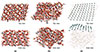 |
Fig. 1. Model dust structure and binding energy calculation sites. Column (a): Unit cell of the optimized FeMgSiO4 periodic slab before the molecular dynamics simulation of heating to 5000 K to amorphize the structure. Column (b): FeMgSiO4 periodic slab structure after amorphization proceedure. Column (c): 81 grid points used in calculating binding energies. |
The periodic slab structure was relaxed to have an energetically favorable configuration using the GFN1-xTB method. The resulting structure was used as the initial configuration for a molecular dynamics simulation at 5000 K. During the molecular dynamics simulation, the atomic positions of the periodic slab structure evolved according to Newton’s equations of motion, enabling the time-dependent structural fluctuations to converge to an equilibrium configuration. We set a relatively high temperature of 5000 K to induce kinetic energy corresponding to that temperature in order to enable the atoms in the crystalline lattice to effectively randomize their positions within a short simulation timescale (1100 fs) and form an amorphous structure.
Statistics of computed binding energy distributions for each element.
In the molecular dynamics simulation, temperature control is essential. For this purpose, the Berendsen thermostat (Berendsen & Postma 1984) was employed, which can maintain the temperature by weakly coupling the simulated system to an external heat bath. Moreover, the thermostat works by scaling the velocities of atoms in the system and allowing the temperature to gradually approach the target temperature. For the molecular dynamics simulation, a timestep of 0.25 fs was used to achieve stable and accurate integration of atomic trajectories. As the simulation progresses, the total energy gradually stabilizes so that from around 700 fs, the temperature oscillates around 5000 K (Fig A.1).
After the molecular dynamics simulation, we performed a static geometry optimization to find a stable configuration, without any temperature control or dynamics. The resulting structure was used as the FeMgSiO4 dust particle model (Figure 1b). After that, 81 uniformly spaced grid points were selected approximately 4 Å above the optimized dust particle model surface (Figure 1c). We chose this distance, as it is longer than the typical interatomic spacing, and thus weak interactions between the atom sitting on the grid and the dust particle guide the atom to find an energy minimum during the geometry optimizations. The binding energy of the atom was computed using the following formula:
 (1)
(1)
In this formula, Edust-atom is the total potential energy of the optimized dust particle with the atom attached to it. The Edust term represents the potential energy of the optimized dust particle model, and Eatom is the potential energy of the atom.
3. Results
3.1. Binding energy distributions
The summary statistics of the binding energy distribution for each element are given in Table 1. The geometries of the optimized local minima of the selected structures are shown in Figure 2. The computed mean binding energies follow the order Si (15.31 eV) > Ca (13.52 eV) > Al (12.79 eV) > C (9.20 eV) > O (8.10 eV) > N (6.37 eV) > Fe (5.92 eV) > S (5.17 eV) > Mg (2.57 eV). Si is typically the most strongly bound atom, while Mg is typically the weakest, although there is substantial spread in the values for any one element.
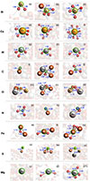 |
Fig. 2. Selected optimized geometries of the local minima corresponding to the weakest, median, and strongest binding energies. The absorbed atom is indicated by a green circle. |
The computed data showed a range of binding energies for Si on the FeMgSiO4 dust particle model, where 10.40 eV is the weakest binding energy and 22.21 eV is the strongest binding energy. The geometries of the local minima suggest that in almost all cases, the Si atom does not stay on the dust particle surface. Instead, the Si atom forms several chemical bonds with the atoms on the surfaces and moves into the dust particle but remains near the surface. The binding energy is the lowest when the Si atom establishes two bonds with the surface O atoms, as we shown in Figure 2a. In Figure 2b, we illustrate the binding site that gives the median binding energy, where the Si atom forms four bonds with the dust particle surface atoms (three O and one Fe). The computed binding energy is the strongest when Si forms four bonds with the surface O atoms, shown in Figure 2c.
In the case of the Ca atom, four to nine chemical bonds can be formed with O atoms on the surface of the dust particle (Figure 2d-f). Thus, the computed binding energies are strong (the weakest binding energy is 10.28 eV, and the strongest binding energy is 22.28 eV). As a result, the Ca atom can also move into the dust particle while also remaining near the surface. The Al atom also showed a relatively strong binding energy, where it can create three chemical bonds with the O atoms of the dust particle (Figure 2g-i). Thus, the Al atom sits either on the surface or goes into the dust particle and stays near the surface.
The C atom establishes chemical bonds with the Fe, Mg, and O atoms on the FeMgSiO4 dust particle surface. The computed binding energy of the C atom is the weakest (4.63 eV) when the C atom interacts with only one Fe (Figure 2j), and the binding energy is the strongest (16.44 eV) when the C atom interacts with two O atoms and one Fe (Figure 2l). The binding energy of the C atom on the surface is relatively weak compared to that of the Si atom, which sits in the same group of the periodic table. This is because C does not bind well into the silicate, while Si can form strong Si-O-Si bonds in the oxygen-rich environment of silicates. In the case of the O atom, the calculated binding energies are in the range of 6.02–12.00 eV, and the computed median binding energy is 8.10 eV. The geometries of the optimized structures suggest that the O atom can create chemical bonds with any atom on the surface (Figure 2m-o). The N atom showed a relatively weak binding energy (3.26–10.60 eV, Figure 2p-r), and it can interact with any atom on the particle surface.
The Fe atom makes bonds with O or Fe on the particle surface. The computed weakest binding energy of the Fe atom is 3.12 eV, where the Fe atom makes bonds with one surface O and one surface Fe (Figure 2s). When the Fe atom makes bonds with three surface O atoms and two surface Fe atoms, the binding energy is the strongest (10.04 eV, Figure 2u). In the case of the S atom, one to three chemical bonds can be made with any atom on the surface (Figure 2v-x), and the calculated binding energies range from 3.21 eV to 10.83 eV. Compared to the O atom, which is in the same group of the periodic table as S, the computed binding energy of the S atom is relatively weak due to differences in electronegativity. Moreover, the atomic radius of O is smaller than that of S, and therefore O makes stronger bonds with the silicate surface. The relatively large atomic radius of a sulfur atom results in weaker orbital overlap with the surface atoms, thereby forming weaker bonds compared to O atoms. The Mg atom either makes no chemical bond with the surface atoms of the FeMgSiO4 dust particle (and is held to the surface by non-covalent interactions, e.g., Figure 2y) or establishes two to four chemical bonds with the O atoms of the surface. In the former case, the binding energy is as low as 1.55 eV, while the binding energy is the strongest when the Mg atom makes four chemical bonds with O on the particle surface (Figure 2z1).
It is important to note that even this weakest binding energy corresponds to a thermal kinetic temperature T = 2Eb/3kB = 1.2 × 10⁴ K, which is much higher than the temperatures reached by dust in almost all astrophysical environments. Thus, the relative differences in binding energies of these atoms do not significantly impact the growth of silicate dust in all but the most extreme astrophysical environments. Therefore, thermal desorption rates are negligibly low for all accreted elements, even Mg, and it is the relative gas-phase abundances and sticking coefficients that should determine the composition of accreted material on the grain surface, except in extreme environments with temperatures comparable to the binding energies (see Sections 3.2 and 4.1).
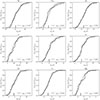 |
Fig. 3. Cumulative distribution functions of binding energies of atoms on the FeMgSiO4 dust particle model. Solid lines are the cumulative distribution functions from the molecular dynamics calculations. Dashed lines are the cumulative distribution functions of the best-fit log-normal distributions, labeled by the Kolmogorov-Smirnov test p-value. The vertical line indicates the exponentiated logarithmic mean. |
Visual inspection of the computed structures confirmed that the C, O, N, and S atoms can form bonds with any atom of the dust particle after adsorption (Table A.1). The Si and Fe atoms can form bonds only with Fe and O atoms of the dust particle, whereas Ca, Al, and Mg atoms can form bonds only with O atoms of the surface upon adsorption.
The computed probability distributions of the binding energies of atoms on the FeMgSiO4 dust particle model are shown in Figure 3, which for all but one element (Ca) are statistically consistent with a log-normal distribution as evaluated by a Kolmogorov-Smirnov test, implemented in the scipy.stats Python library (Virtanen et al. 2020). This is perhaps surprising, as one could imagine that the finite number of bond types possible for each element would result in characteristic values of the binding energy distribution that would make it more complicated. However, it appears that the amorphous nature of the grain model used in the calculations results in a sufficient variety of bonding configurations for each element such that the central limit theorem approximately holds. This may also reflect the relative insensitivity of the Kolmogorov-Smirnov test to distribution details or to the small number of binding sites in our sample.
3.2. Sublimation temperatures
The binding energies computed in this study determine the rate of thermal desorption from the grain into the gas phase (i.e., a sublimation rate). In this section, we are interested in the time it takes for the grains of a finite temperature to completely sublimate (i.e., completely evaporate), and we refer to that as sublimation. Thus, a given (non-zero) lifetime for a grain specifies a sublimation temperature. One must therefore specify both a grain size and a grain lifetime to define a sublimation temperature. Of course, this is an approximation assuming that the grain remains at the same temperature for its entire lifetime and that the binding energy distributions of its surface atoms remain the same, which is not realistic in detail but a reasonable way to proceed. These temperatures are approximate values meant to give a scale for the temperatures above which a grain will be unstable to thermal sublimation, and more precise calculations should include these other dynamical effects. To predict grain sublimation temperatures, we began with the mass flux of grains due to thermal desorption from the surface given by the Polanyi-Wigner equation (Polanyi & Wigner 1928; Potapov et al. 2018):
 (2)
(2)
where i indexes all the elements of which the grain is composed, Ni is the number of each element on the surface, ν0, i is the characteristic vibration frequency of each element, Ui is the surface binding energy of each element (here assumed to be constant for all atoms of the same element), and T is the dust grain temperature. We can express the number of atoms of each element on the surface as
 (3)
(3)
where ρg is the grain material density, fi is the mass fraction of each constituent element given by
 (4)
(4)
and vmono, the volume of the surface “monolayer” (the layer with atoms capable of escaping from the surface), is
 (5)
(5)
Here, ⟨x⟩ is the average monolayer thickness (assumed ≪ a) defined by
 (6)
(6)
where Nmono, i is the number of elements, i, in each monolayer “unit”, each with a characteristic size, xi. For the assumed chemical composition of our silicate grain, Nmono, Fe = Nmono, Mg = Nmono, Si = 1 and Nmono, O = 4. Note that we can relate this to the grain material density, ρg, as follows:
 (7)
(7)
giving
![Mathematical equation: $$ \begin{aligned} \frac{dm_g}{dt} = -4\pi a^2\rho _g\left(\frac{\sum _i N_{\mathrm{{mono}},i}m_i}{\rho _g}\right)^{1/3}\left[\sum _i f_i\nu _{0,i}\exp \left(\frac{-U_i}{k_{\rm {B}}T}\right)\right]. \end{aligned} $$](/articles/aa/full_html/2026/03/aa56997-25/aa56997-25-eq8.gif) (8)
(8)
This mass evolution equation can be reexpressed in terms of the rate of change of the grain’s effective radius, a:
 (9)
(9)
We note that in the above equation, we assume a constant ρg, which is incorrect in principle because more weakly bound elements will desorb more quickly and change the grain composition on the surface, but we ignore this effect because it is negligible for grains with sizes much larger than a single monolayer. Our grain radius evolution equation is then
![Mathematical equation: $$ \begin{aligned} \frac{da}{dt} = -\left(\frac{\sum _i N_{\mathrm{{mono}},i}m_i}{\rho _g}\right)^{1/3}\left[\sum _i f_i\nu _{0,i}\exp \left(\frac{-U_i}{k_{\rm B}T}\right)\right]. \end{aligned} $$](/articles/aa/full_html/2026/03/aa56997-25/aa56997-25-eq10.gif) (10)
(10)
However, this expression assumes that all atoms of a given element, i, have the same surface binding energy, Ui, which we predict from our calculations is not strictly correct. To account for a probability distribution function of binding energies for a given atom P(Ui), we replaced the Boltzmann factor by its expectation value over this distribution:
 (11)
(11)
thus ultimately giving us
![Mathematical equation: $$ \begin{aligned} \frac{da}{dt} = -\left(\frac{\sum _i N_{\mathrm{{mono}},i}m_i}{\rho _g}\right)^{1/3}\left[\sum _i f_i\nu _{0,i}\left\langle \exp \left(\frac{-U_i}{k_{\rm {B}}T}\right)\right\rangle \right]. \end{aligned} $$](/articles/aa/full_html/2026/03/aa56997-25/aa56997-25-eq12.gif) (12)
(12)
However, this equation only holds for desorption of the most loosely bound atoms in the first monolayer. The sublimation thereafter will be rate-limited by the most strongly bound element, in our case Si. Therefore, the long-term grain radius evolution differential equation will be
 (13)
(13)
To estimate grain lifetimes Δtsubl or, equivalently, the sublimation temperatures Tsubl, assuming T in Eq. (12) does not evolve with time or grain radius allows this differential equation to be integrated trivially to obtain
![Mathematical equation: $$ \begin{aligned} \Delta t_{\rm {subl}}(a, T) = a \left(\frac{\sum _i N_{\mathrm{{mono}},i}m_i}{\rho _g}\right)^{-1/3}\left[\nu _{0,\mathrm{{Si}}}\left\langle \exp \left(\frac{-U_{\rm {Si}}}{k_{\rm B}T}\right)\right\rangle \right]^{-1} \end{aligned} $$](/articles/aa/full_html/2026/03/aa56997-25/aa56997-25-eq14.gif) (14)
(14)
for the grain lifetime Δtsubl as a function of grain radius and temperature or, alternatively, to define the sublimation temperature, Tsubl(a|Δt), at a given grain radius and lifetime by
 (15)
(15)
While Tsubl(a|Δt) precludes a symbolic expression, this equation can be solved for T numerically.
The predicted values of Tsubl(a|Δt) obtained from the numerical solution of Eq. (15) combined with the binding energy distribution of Si, for the relevant range of a and Δt, are shown in Fig. 4. In this calculation we assumed a temperature-dependent vibrational frequency for silicon bonds, described in Appendix B. Because of this, we subtracted a zero-point energy of 0.2 eV from the Si binding energy distribution. We also adopted a grain material density of ρg = 3.32g cm−3 for olivine.1 To estimate the probability distribution function, Pi(U), for each element from the molecular dynamics calculations, we employed a kernel density estimate with the Epanechnikov kernel of constant size set to the optimal value using Silverman’s “rule-of-thumb” (Silverman 1986). Sublimation temperatures range from ≈1600 K to ≈3000 K depending on assumed grain size and lifetime and are approximately consistent with previous estimates in the literature (Pollack et al. 1994; Waxman & Draine 2000) as well as temperatures of dust observed in active galactic nucleus environments (Barvainis 1987; Kishimoto et al. 2007). We note that in principle, the compositional changes due to different thermal desorption rates for different elements will likely change the binding energy distribution as the desorption goes on. However, we expect that these changes will not be so large as to qualitatively change our conclusions. This is partly helped by the grain being amorphous, which should facilitate the rearrangement of bonds so that they remain statistically similarly distributed as the grain sublimates.
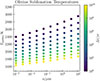 |
Fig. 4. Sublimation temperatures for silicate dust calculated from binding energy distributions. |
We note that since we used binding energies for individual atoms in our calculations, we assumed that these will be the products of the thermal desorption (i.e., individual Si, O, Fe, and Mg atoms) returned to the ISM. In principle, determining these products would require additional computations (which is beyond of the scope of this manuscript) as well as employing a more sophisticated simulation technique than our simple symbolically expressible model in Eq. (14).
4. Discussion
4.1. Consistency with observed temperatures
The sublimation temperatures shown in Fig. 4 are much higher than typical temperatures of dust in the ambient ISM, confirming the standard assumption that thermal desorption is generally unimportant for dust grain evolution in these environments, and these grains are stable to thermal sublimation on cosmological timescales. However, these values are comparable to or much higher than the observed or predicted temperatures of dust in the most extreme interstellar environments: asymptotic giant branch stars (e.g., Lorenz-Martins & Pompeia 2000; Suh 2004; Lagadec et al. 2005; Heras & Hony 2005; Groenewegen et al. 2009; Goldman et al. 2017; Höfner et al. 2022), supernova remnants (see Micelotta et al. 2018), and the dusty tori of active galactic nuclei (e.g., Barvainis 1987; Oyabu et al. 2011; GRAVITY Collaboration 2020; Nenkova et al. 2008; Netzer 2015; Weigelt et al. 2012; Sakamoto et al. 2021). Therefore, these values will enable the precise calculation of grain growth and destruction rates in the full variety of interstellar environments that they experience.
4.2. Comparison with photon energies in the interstellar radiation field
For every element considered except Si, the average binding energy is lower than 13.6 eV, indicating that there are abundant photons in the diffuse ISM of similar or higher energies. However, we do not believe the process of photodesorption – wherein an impacting photon excites a bonded atom on the surface of the grain such that it is desorbed – to be a prominent mechanism of insterstellar grain destruction. This is because such photodesorption would require a significant fraction of the photon energy to be concentrated in the bond(s) attaching the surface atom to the substrate, which should have a relatively low probability compared to the excitation of the many other electronic, thermal, and vibrational degrees of freedom of the surrounding atoms, especially in grains of more than a few atoms. Indeed, Guhathakurta & Draine (1989) found that silicate particles with greater than 37 atoms, corresponding to a radius of 4.3Å, are stable to the diffuse ISM radiation field.
4.3. Implications of carbon and oxygen binding energies: SiC dust and SiO or SiO2 formation
The binding energies of carbon atoms are of particular interest because interstellar dust is often assumed to consist of two separate chemical species, one that is primarily (hydro)carbonaceous and the other being silicates, which are the focus of this study (see Draine 2011, and references therein). The ability of carbon to bond to the silicate substrate, as predicted by our calculations, challenges this canonical chemical dichotomy.
Our calculated binding energies of carbon atoms are also interesting in the context of the apparently minimal contribution of SiC to nearby interstellar dust: existing constraints prefer either a small fraction (a few percent; Min et al. 2007) or place only upper limits on (Chiar & Tielens 2006; Whittet et al. 1990) the mass fraction of cosmic dust composed of SiC along several galactic sight lines. Chemisputtering, wherein any accreted C atom is promptly removed by forming a molecule with O (for example), is a possible explanation, but it appears to be inadequately efficient (Chen et al. 2022). However, it should be noted that Decleir et al. (2025) find what might be tentative evidence for SiC in many more sight lines through the diffuse medium in the form of enhanced opacity between 11μm and 12μm, an optical feature that has been used to unambiguously identify silicon carbide in asymptotic giant branch star outflows (e.g., Speck et al. 1997), even at low metallicities (Boyer et al. 2025). Moreover, this compound has been identified in meteorites that are possibly of pre-solar origin (Bernatowicz et al. 1987). Finally, it should be emphasized that there are significant uncertainties in the material properties of grains inferred from observations of the local ISM, not to mention their possible variations in different environments throughout the Universe. All of this is to say that the SiC dust fraction might be small but nonzero in the very local ISM and is largely unconstrained elsewhere.
Moreover, we emphasize that the strong binding energies of carbon to silicates is a necessary but not sufficient condition for the presence of SiC dust in the Universe (as is true for any other compound that might form on dust surfaces). Given the complexity of physical and chemical processes to which grains are subject to in the ISM, it is impossible to make a definitive statement on any potential discrepancy with observational estimates because the number of atoms of a given element that stick to a dust grain surface is dependent on not only the binding energy (which is what this study probes) but also the fraction that sticks in the first place (i.e., the sticking coefficient, Bossion et al. 2024), the geometry of the grain, the local abundance ratios in the gas phase of the ISM, the catalysis and desorption possible from interactions with the radiation field, chemisputtering (Chen et al. 2022), and the fraction of the dust surface that is covered in a nonreactive “ice” mantle, none of which this study can explicitly address. A full assessment of the ability of carbon atoms to bond to and participate in the growth of silicate dust will require further work on and a simultaneous accounting of these physical processes.
We note that the stronger binding energies of O than Fe or Mg imply that, in principle, the accretion of silicon atoms could result in the formation of SiO or SiO2 molecules on the surface of silicate interstellar gains. These molecules may desorb. A comprehensive computational investigation will be necessary to obtain detailed insights, and this will be the focus of our future work. Regardless, the similarity of the spectral features characteristic of these molecules and Si-O bonds in larger silicates would be difficult to distinguish observationally.
4.4. Implications of sulfur binding energies: A possible reservoir
The depletion of sulfur from the gas phase in the ISM is not yet understood (see Yang et al. 2024, and refs. therein). Despite being on average the second-weakest bound element in our calculations, stronger only than Mg, the ∼5 eV binding energy characteristic of sulfur atoms suggest that it can in principle bind to the surfaces of silicate dust grains. Future work should therefore be dedicated to determining the characteristic optical properties of such a dust composition and searching for these in observational data if possible.
4.5. Implications of N binding energies
The binding energies of nitrogen suggest that it can also, in principle, stick to amorphous silicate dust grains. This is possibly in contradiction with the observational result that nitrogen is not strongly depleted from the gas phase of the ISM (Jenkins 2009), though depletion measurements have large uncertainties. The binding energies we find may require the revision of existing dust models (e.g., Jones et al. 2013; Hensley & Draine 2023) to account for the possibility of nitrogen inclusion in candidate grain materials or may point to some process – such as the chemisputtering of N from grain surfaces due to the formation of N2 – that prevents the incorporation of large amounts of N into dust. Further work on this issue is needed.
5. Conclusions
In this work, we computed the binding energies of C, O, Mg, Si, S, Al, Ca, Fe, and Ni atoms on a FeMgSiO4 periodic dust particle model surface using the GFN1-xTB method. The GFN1-xTB approach has been shown to provide reliable and computationally efficient results for complex molecular systems. The computed data showed a range of binding energies for each atom. The mean of the binding energies follows the order Si (15.3 eV) > Ca (13.5 eV) > Al (12.8 eV) > C (9.2 eV) > O (8.1 eV) > N (6.4 eV) > Fe (5.9 eV) > S (5.2 eV) > Mg (2.6 eV). At the present level of theory, the Si and Ca atoms can react with the surface, giving rise to several chemical bonds between each atom (Si or Ca) and the particle surface atoms. In our simulations, the Si and Ca atoms penetrate into the FeMgSiO4 dust particle but stay near the particle surface (i.e., they do not stay on the surface). Other atoms are adsorbed on the FeMgSiO4 dust particle and sit on the particle surface. We found log-normal binding energy distributions for most elements, and we used these distributions to estimate sublimation temperatures for silicate dust grains, which are consistent with observations and previous theoretical estimates. These unprecedentedly precise characterizations of silicate dust surface chemical properties will enable accurate calculations of dust processes in the full diversity of ISM environments and thus sophisticated predictions about the interplay between ISM dynamics and dust evolution.
Acknowledgments
We acknowledge support from the Knut and Alice Wallenberg Foundation under grant no. KAW 2020.0081. Supercomputing resources provided by Chalmers e-Commons at Chalmers and the National Academic Infrastructure for Supercomputing in Sweden (NAISS), partially funded by the Swedish Research Council through grant agreement no. 2022-06725. We thank Theo Khouri for providing references on asymptotic giant branch star dust temperatures. We thank the anonymous referee for a careful review and alerting us to relevant literature.
References
- Barvainis, R. 1987, ApJ, 320, 537 [Google Scholar]
- Berendsen, H. J., Postma, J. V., Van Gunsteren, W. F., DiNola, A., & Haak, J. R., 1984, J. Chem. Phys., 81, 3684 [NASA ADS] [CrossRef] [Google Scholar]
- Bernatowicz, T., Fraundorf, G., Ming, T., et al. 1987, Nature, 330, 728 [Google Scholar]
- Bossion, D., Sarangi, A., Aalto, S., et al. 2024, A&A, 692, A249 [NASA ADS] [CrossRef] [EDP Sciences] [Google Scholar]
- Boyer, M. L., Sloan, G. C., Nanni, A., et al. 2025, ApJ, 991, 24 [Google Scholar]
- Cecchi-Pestellini, C., Casu, S., Mulas, G., & Zonca, A. 2014a, ApJ, 785, 41 [CrossRef] [Google Scholar]
- Cecchi-Pestellini, C., Viti, S., & Williams, D. A. 2014b, ApJ, 788, 100 [Google Scholar]
- Chatterjee, S., Sengupta, S., Saha-Dasgupta, T., Chatterjee, K., & Mandal, N. 2009, Phys. Rev. B, 79, 115103 [Google Scholar]
- Chen, T., Xiao, C. Y., Li, A., & Zhou, C. T. 2022, MNRAS, 509, 5231 [Google Scholar]
- Chiar, J. E., & Tielens, A. G. G. M. 2006, ApJ, 637, 774 [NASA ADS] [CrossRef] [Google Scholar]
- Compiègne, M., Verstraete, L., Jones, A., et al. 2011, A&A, 525, A103 [Google Scholar]
- Decleir, M., Gordon, K. D., Misselt, K. A., et al. 2025, AJ, 169, 99 [Google Scholar]
- Demyk, K., Jones, A., Dartois, E., Cox, P., & d’Hendecourt, L. 1999, A&A, 349, 267 [Google Scholar]
- Desert, F.-X., Boulanger, F., & Puget, J. 1990, A&A, 237, 215 [NASA ADS] [Google Scholar]
- Do-Duy, T., Wright, C. M., Fujiyoshi, T., et al. 2020, MNRAS, 493, 4463 [Google Scholar]
- Draine, B. T. 1990, in The Evolution of the Interstellar Medium, ed. L. Blitz, ASP Conf. Ser., 12, 193 [Google Scholar]
- Draine, B. T. 2003, ARA&A, 41, 241 [NASA ADS] [CrossRef] [Google Scholar]
- Draine, B. T. 2009, in Cosmic Dust - Near and Far, eds. T. Henning, E. Grün, & J. Steinacker, ASP Conf. Ser., 414, 453 [NASA ADS] [Google Scholar]
- Draine, B. T. 2011, Physics of the Interstellar and Intergalactic Medium (Princeton, NJ: Princeton University Press) [Google Scholar]
- Draine, B., & Hensley, B. S. 2021, ApJ, 909, 94 [NASA ADS] [CrossRef] [Google Scholar]
- Draine, B., & Lee, H. M. 1984, ApJ, 285, 89 [NASA ADS] [CrossRef] [Google Scholar]
- Draine, B., & Li, A. 2001, ApJ, 551, 807 [NASA ADS] [CrossRef] [Google Scholar]
- Draine, B. T., & Li, A. 2007, ApJ, 657, 810 [CrossRef] [Google Scholar]
- Duley, W. 1987, MNRAS, 229, 203 [Google Scholar]
- Duley, W., Jones, A., & Williams, D. 1989, MNRAS, 236, 709 [Google Scholar]
- Dullemond, C. P., & Monnier, J. D. 2010, ARA&A, 48, 205 [NASA ADS] [CrossRef] [Google Scholar]
- Dwek, E., Arendt, R., Fixsen, D., et al. 1997, ApJ, 475, 565 [NASA ADS] [CrossRef] [Google Scholar]
- Esmerian, C. J., & Gnedin, N. Y. 2022, ApJ, 940, 74 [NASA ADS] [CrossRef] [Google Scholar]
- Esmerian, C. J., & Gnedin, N. Y. 2024, ApJ, 968, 113 [NASA ADS] [CrossRef] [Google Scholar]
- Fogerty, S., Forrest, W., Watson, D. M., Sargent, B. A., & Koch, I. 2016, ApJ, 830, 71 [NASA ADS] [CrossRef] [Google Scholar]
- Gilman, R. C. 1969, ApJ, 155, L185 [Google Scholar]
- Goldman, S. R., van Loon, J. T., Zijlstra, A. A., et al. 2017, MNRAS, 465, 403 [Google Scholar]
- GRAVITY Collaboration (Dexter, J., et al.) 2020, A&A, 635, A92 [NASA ADS] [CrossRef] [EDP Sciences] [Google Scholar]
- Greenberg, J. 1986, Ap&SS, 128, 17 [Google Scholar]
- Greenberg, J. M., & Chlewicki, G. 1983, ApJ, 272, 563 [Google Scholar]
- Grimme, S., Bannwarth, C., & Shushkov, P. 2017, J. Chem. Theory Comput., 13, 1989 [Google Scholar]
- Groenewegen, M. A. T., Sloan, G. C., Soszyński, I., & Petersen, E. A. 2009, A&A, 506, 1277 [NASA ADS] [CrossRef] [EDP Sciences] [Google Scholar]
- Guhathakurta, P., & Draine, B. T. 1989, ApJ, 345, 230 [NASA ADS] [CrossRef] [Google Scholar]
- Hensley, B. S., & Draine, B. T. 2023, ApJ, 948, 55 [Google Scholar]
- Heras, A. M., & Hony, S. 2005, A&A, 439, 171 [NASA ADS] [CrossRef] [EDP Sciences] [Google Scholar]
- Höfner, S., Bladh, S., Aringer, B., & Eriksson, K. 2022, A&A, 657, A109 [NASA ADS] [CrossRef] [EDP Sciences] [Google Scholar]
- Hoyle, F., & Wickramasinghe, N. C. 1962, MNRAS, 124, 417 [NASA ADS] [CrossRef] [Google Scholar]
- Hoyle, F., & Wickramasinghe, N. C. 1969, Nature, 223, 459 [Google Scholar]
- Jenkins, E. B. 2009, ApJ, 700, 1299 [Google Scholar]
- Jones, A. 1990, MNRAS, 247, 305 [NASA ADS] [Google Scholar]
- Jones, A., Greenberg, W., & Williams, D. 1987, MNRAS, 229, 213 [Google Scholar]
- Jones, A., Duley, W., & Williams, D. 1990, Roy. Astron. Soc., Quart. J., 31, 567 [Google Scholar]
- Jones, A., Fanciullo, L., Köhler, M., et al. 2013, A&A, 558, A62 [NASA ADS] [CrossRef] [EDP Sciences] [Google Scholar]
- Jones, A. P., Ysard, N., Köhler, M., et al. 2014, Faraday Discuss., 168, 313 [Google Scholar]
- Jones, A., Köhler, M., Ysard, N., et al. 2016, A&A, 588, A43 [NASA ADS] [CrossRef] [EDP Sciences] [Google Scholar]
- Kamijo, F. 1963, PASJ, 15, 440 [Google Scholar]
- Kemper, F., Vriend, W. J., & Tielens, A. G. G. M. 2005, ApJ, 633, 534 [Google Scholar]
- Kishimoto, M., Hönig, S. F., Beckert, T., & Weigelt, G. 2007, A&A, 476, 713 [NASA ADS] [CrossRef] [EDP Sciences] [Google Scholar]
- Köhler, M., Jones, A., & Ysard, N. 2014, A&A, 565, L9 [NASA ADS] [CrossRef] [EDP Sciences] [Google Scholar]
- Kramida, A., Ralchenko, Y., Reader, J., & NIST ASD Team, 2024, NIST Atomic Spectra Database (Version 5.12) [Google Scholar]
- Lagadec, E., Mékarnia, D., de Freitas Pacheco, J. A., & Dougados, C. 2005, A&A, 433, 553 [NASA ADS] [CrossRef] [EDP Sciences] [Google Scholar]
- Li, A., & Draine, B. 2001, ApJ, 554, 778 [NASA ADS] [CrossRef] [Google Scholar]
- Li, A., & Draine, B. T. 2001, ApJ, 550, L213 [NASA ADS] [CrossRef] [Google Scholar]
- Li, A., & Draine, B. 2002, ApJ, 576, 762 [Google Scholar]
- Li, A., & Greenberg, J. M. 1997, A&A, 566 [Google Scholar]
- Li, M. P., Zhao, G., & Li, A. 2007, MNRAS, 382, L26 [NASA ADS] [Google Scholar]
- Lira, P., Videla, L., Wu, Y., et al. 2013, ApJ, 764, 159 [Google Scholar]
- Lorenz-Martins, S., & Pompeia, L. 2000, MNRAS, 315, 856 [Google Scholar]
- Mathis, J. S., Rumpl, W., & Nordsieck, K. H. 1977, ApJ, 217, 425 [Google Scholar]
- Micelotta, E. R., Matsuura, M., & Sarangi, A. 2018, Space Sci. Rev., 214, 53 [NASA ADS] [CrossRef] [Google Scholar]
- Min, M., Waters, L. B. F. M., de Koter, A., et al. 2007, A&A, 462, 667 [NASA ADS] [CrossRef] [EDP Sciences] [Google Scholar]
- Nenkova, M., Sirocky, M. M., Ivezić, Ž., & Elitzur, M. 2008, ApJ, 685, 147 [Google Scholar]
- Netzer, H. 2015, ARA&A, 53, 365 [Google Scholar]
- Oort, J., & Van de Hulst, H. 1946, Bull. Astron. Inst. Neth., 10, 187 [Google Scholar]
- Oyabu, S., Ishihara, D., Malkan, M., et al. 2011, A&A, 529, A122 [NASA ADS] [CrossRef] [EDP Sciences] [Google Scholar]
- Pitt, I. G., Gilbert, R. G., & Ryan, K. R. 1994, J. Phys. Chem. A, 98, 13001 [Google Scholar]
- Polanyi, M., & Wigner, E. 1928, Z. Phys. Chem. A, 139, 439 [Google Scholar]
- Pollack, J. B., Hollenbach, D., Beckwith, S., et al. 1994, ApJ, 421, 615 [Google Scholar]
- Potapov, A., Jäger, C., & Henning, T. 2018, ApJ, 865, 58 [NASA ADS] [CrossRef] [Google Scholar]
- Poteet, C. A., Whittet, D. C. B., & Draine, B. T. 2015, ApJ, 801, 110 [NASA ADS] [CrossRef] [Google Scholar]
- Sakamoto, K., González-Alfonso, E., Martín, S., et al. 2021, ApJ, 923, 206 [NASA ADS] [CrossRef] [Google Scholar]
- Siebenmorgen, R., & Krügel, E. 1992, A&A, 259, 614 [Google Scholar]
- Siebenmorgen, R., Voshchinnikov, N., & Bagnulo, S. 2014, A&A, 561, A82 [NASA ADS] [CrossRef] [EDP Sciences] [Google Scholar]
- Silverman, B. W. 1986, Density Estimation for Statistics and Data Analysis (London: Chapman and Hall) [Google Scholar]
- Sorrell, W. H. 1991, MNRAS, 248, 439 [NASA ADS] [Google Scholar]
- Speck, A. K., Barlow, M. J., & Skinner, C. J. 1997, MNRAS, 288, 431 [Google Scholar]
- Suh, K.-W. 2004, ApJ, 615, 485 [Google Scholar]
- Tait, S. L., Dohnálek, Z., Campbell, C. T., & Kay, B. D. 2005, J. Chem. Phys., 122, 164708 [NASA ADS] [CrossRef] [Google Scholar]
- Te Velde, G. T., Bickelhaupt, F. M., Baerends, E. J., et al. 2001, J. Comput. Chem., 22, 931 [Google Scholar]
- van de Hulst, H. 1943, Ned. Tijdschr. v. Natuurkunde, 10, 251 [Google Scholar]
- Virtanen, P., Gommers, R., Oliphant, T. E., et al. 2020, Nat. Methods, 17, 261 [Google Scholar]
- Wang, S., Li, A., & Jiang, B. W. 2015, ApJ, 811, 38 [NASA ADS] [CrossRef] [Google Scholar]
- Waxman, E., & Draine, B. T. 2000, ApJ, 537, 796 [NASA ADS] [CrossRef] [Google Scholar]
- Weigelt, G., Hofmann, K. H., Kishimoto, M., et al. 2012, A&A, 541, L9 [NASA ADS] [CrossRef] [EDP Sciences] [Google Scholar]
- Whittet, D. C. B., Duley, W. W., & Martin, P. G. 1990, MNRAS, 244, 427 [NASA ADS] [Google Scholar]
- Wickramasinghe, N. C. 1963, MNRAS, 126, 99 [Google Scholar]
- Xie, Y., Li, A., & Hao, L. 2017, ApJS, 228, 6 [Google Scholar]
- Yang, X. J., Hua, L., & Li, A. 2024, ApJ, 974, 30 [NASA ADS] [CrossRef] [Google Scholar]
- Ysard, N., Köhler, M., Jones, A., et al. 2015, A&A, 577, A110 [NASA ADS] [CrossRef] [EDP Sciences] [Google Scholar]
- Ysard, N., Köhler, M., Jones, A., et al. 2016, A&A, 588, A44 [NASA ADS] [CrossRef] [EDP Sciences] [Google Scholar]
- Zonca, A., Cecchi-Pestellini, C., Mulas, G., & Malloci, G. 2011, MNRAS, 410, 1932 [NASA ADS] [Google Scholar]
Appendix
In Fig A.1. the molecular dynamics simulation results show a typical equilibration behavior of the system. Initially both the total energy and the temperature increase sharply, suggesting that the system is relaxing from the initial configuration. As the simulation progresses, the total energy gradually stabilizes, while the temperature oscillates around 5000 K. Table A.1 summarizes the interactions between adsorbed atoms and dust particle surfaces.
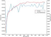 |
Fig. A.1. Total energy and temperature profiles during molecular dynamics simulation to amorphize molecular structure. |
Interaction of adsorbed atoms with dust particle surface.
Energy (AU) of the optimized local minima
Energy (AU) of the optimized local minima ( Continue....)
Appendix
To calculate estimates of the frequency factor (preexponential factor) for the desorption rate coefficient expression we have employed Transition State Theory (TST) (Pitt et al. 1994; Tait et al. 2005). The system is divided into the atom that is desorbing and the rest of the grain. The basic expression for the desorption rate constant is
 (B.1)
(B.1)
where Edes is the desorption energy from a binding site. The temperature, T, is the temperature of the grain surface. If there is no additional energy barrier to desorption Edes = Ebind. QR and Q‡ are the partition functions of the reactant state and transition state, respectively. With this definition the pre-exponential factor can be identified as the frequency factor in the Polanyi-Wigner expression. It should be borne in mind that the TST expression is in general an upper bound of the real rate constant if all interactions are treated with the highest accuracy possible.
The definition of the reactant state and transition state is not unambiguous. For a strongly bonded atom at a surface it is natural to take the reactant state to be represented by the atom localized at a specific location and its motion in three degrees of freedom will be characterized by three vibrational frequencies. As the atom gains more kinetic energy, its motion could eventually be characterized as two-dimensional (hindered) translation parallel to the surface and one-dimensional vibration in the direction normal to the surface. The transition state can be taken to occur on a dividing surface at a distance from the surface where the atom-surface interaction is insignificant. At that point motion normal to the surface is now translation in 1D that characterizes motion through the dividing surface, i.e., effectively desorption.
The transition state is characterized by translational motion in 2D, and its extent parallel to the surface is usually taken to be the inverse of the surface binding site density, i.e., an effective area of the binding site. The atom at the transition state is effectively in the gas phase and its electronic degrees of freedom are therefore characterized by its electronic fine-structure states. For the adsorbed atom, the nature of its electronic state is not as clear since its electronic structure is not independent from the other atoms in the surface and it is not in a spherically symmetric environment. A choice can be made to assign its electronic spin multiplicity as the number of electronic states at the surface. The spin multiplicity for the single atom is however not necessarily well-characterized, but lacking more detailed information on the electronic structure it seems like a reasonable approximation.
Given the above information the partition function for the transition state in the expression for the rate constant can be expressed as
 (B.2)
(B.2)
where
 (B.3)
(B.3)
where m is the mass of the atom and A is the typical area of the binding site as discussed above. The electronic partition function is expressed as
 (B.4)
(B.4)
where the sum covers all available electronic fine-structure (spin-orbit) states i of the atom with energies Ei and degeneracy gi.
The corresponding partition function for the reactant state is expressed as
 (B.5)
(B.5)
where the vibrational partition function is taken to be that of the collection of harmonic oscillators describing the three vibrational degrees of freedom of the atom at the surface is:
 (B.6)
(B.6)
Note that the zero of energy is taken with vibrational zero-point energy taken into account. The electronic partition function taken to be the electronic spin multiplicity of the atom at the surface is:
 (B.7)
(B.7)
where S is the total spin quantum number.
In our case the fine-structure energy levels discussed above are taken from high-accuracy experimental data (Kramida et al. 2024) and all levels below a wavenumber of 25000 cm−1 above the electronic ground state are included. The typical area of a binding site is for all species assumed to be 0.2 nm2, which seems like a reasonable estimate. The vibrational modes of the atom at the surface can be quite different depending on the type of binding. In our case a simple approximation has been used where all three frequencies are the same for each atom and it is also assumed that the force constant is the same for all atoms, meaning that relative magnitudes of frequencies between different atoms are proportional to the inverse of the square root of the mass ratio between the atoms.
For Si typical vibrational frequencies are taken to have a wavenumber of 1000 cm−1, and for example Fe vibrations will then have wavenumbers of 707 cm−1 and C vibrations will have 1527 cm−1. Upon desorption it is assumed that the remaining vibrational frequencies of the grain surface remain the same. Both this and the magnitude of the frequencies are relatively crude approximations that could be addressed with detailed analyses of vibrational frequencies. At this point, this introduces a level of complexity that is not really motivated considering other approximations in the models that have been employed.
The multiplicities of the atoms at the surface have been taken to be the same as that of the gas-phase ground state. This means that for instance C, O, Si, and S atoms will have 2S + 1 = 3 (triplet state) and N atoms 2S + 1 = 4 (quartet state). It could be argued that those atoms probably form more strongly bound singlet and doublet states at the surface, respectively. This effort is also not motivated given the other uncertainties in the model. In the present manuscript, we did not take the spin polarization of the system into account. Obtaining a proper description of the electronic state of the reactant would require a detailed analysis of the electronic structure of the grain surface, which lies beyond the scope of this study. It should be mentioned that the actual rate of desorption, and thereby the frequency factor, will be affected by the rates of any transitions between electronic states that might be necessary as the atom leaves the grain surface. Including those effects would effectively lower the predicted desorption rate constants. Such detailed treatments are beyond the scope of the present study and it seems safe to conclude that the frequency factors calculated by the above procedure should be taken as an upper bound. These frequency factors are shown in Fig. B.1.
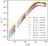 |
Fig. B.1. Desorption frequency factors and zero-point energies. |
All Tables
All Figures
|
Fig. 1. Model dust structure and binding energy calculation sites. Column (a): Unit cell of the optimized FeMgSiO4 periodic slab before the molecular dynamics simulation of heating to 5000 K to amorphize the structure. Column (b): FeMgSiO4 periodic slab structure after amorphization proceedure. Column (c): 81 grid points used in calculating binding energies. |
| In the text | |
|
Fig. 2. Selected optimized geometries of the local minima corresponding to the weakest, median, and strongest binding energies. The absorbed atom is indicated by a green circle. |
| In the text | |
|
Fig. 3. Cumulative distribution functions of binding energies of atoms on the FeMgSiO4 dust particle model. Solid lines are the cumulative distribution functions from the molecular dynamics calculations. Dashed lines are the cumulative distribution functions of the best-fit log-normal distributions, labeled by the Kolmogorov-Smirnov test p-value. The vertical line indicates the exponentiated logarithmic mean. |
| In the text | |
|
Fig. 4. Sublimation temperatures for silicate dust calculated from binding energy distributions. |
| In the text | |
|
Fig. A.1. Total energy and temperature profiles during molecular dynamics simulation to amorphize molecular structure. |
| In the text | |
|
Fig. B.1. Desorption frequency factors and zero-point energies. |
| In the text | |
Current usage metrics show cumulative count of Article Views (full-text article views including HTML views, PDF and ePub downloads, according to the available data) and Abstracts Views on Vision4Press platform.
Data correspond to usage on the plateform after 2015. The current usage metrics is available 48-96 hours after online publication and is updated daily on week days.
Initial download of the metrics may take a while.