© The Authors 2026

1 Introduction

Our knowledge of Jupiter’s interior has been gradually established through bulk and external observables such as mass, radius, atmospheric composition and structure, gravity field, and magnetic field (Fortney & Nettelmann 2010; Guillot 2005). Before any spacecraft reached Jupiter, Jeffreys (1924) first confirmed that Jupiter’s outer region was composed of hydrogen and helium by analyzing the normalized moment of inertia. Building upon the established preponderance of hydrogen in Jupiter’s composition (Wildt 1947), Demarcus (1958) further proposed Jupiter’s interior models featuring a dense central core (~2% M_J) enveloped by hydrogen and helium. Given the observational limitations at the time, the prevailing models generally regarded Jupiter as a relatively cold interior. This hypothesis was refuted by infrared observations (Low 1966), which revealed Jupiter’s internal heat sources and confirmed its fluid nature. Subsequently, Hubbard (1968, 1969) introduced deep convection as the mechanism governing Jupiter’s interior structure and heat transport, analogizing the physical framework outlined by Peebles (1964). Although observations constrain Jupiter’s interior models, interpreting Jupiter’s interior requires a precise understanding of hydrogen’s properties under high pressure. Wigner & Huntington (1935) suspected the existence of a metallic form for hydrogen; that is, hydrogen molecules would dissociate and transform into alkali metals under high pressure. Smoluchowski (1967) and Salpeter (1973) hypothesized that helium immiscibility within metallic hydrogen could lead to helium rain, a process invoked to explain Jupiter’s excess internal heat. This mechanism was later confirmed when the Galileo entry probe directly observed the helium depletion in Jupiter’s atmosphere (Von Zahn et al. 1998). For decades, our understanding of Jupiter’s interior has been primarily shaped by a canonical framework that includes a dense core, a helium-rich metallic hydrogen envelope, and a helium-poor molecular hydrogen atmosphere (Guillot 1999; Saumon & Guillot 2004; Nettelmann et al. 2012; Militzer & Hubbard 2013; Vazan et al. 2015; Miguel et al. 2016; Kong et al. 2016; Ni 2018). This established paradigm was challenged following the arrival of the Juno spacecraft in 2016. The Juno gravity field measurements, especially the high-order harmonics J₄–J₈ (Bolton et al. 2017; Iess et al. 2018), have provided unprecedented constraints that both refine and challenge our understanding of Jupiter’s interior. In order to interpret the Juno gravitational harmonics, Wahl et al. (2017) proposed the inclusion of a diluted core region between the dense core and the metallic hydrogen envelope in the original three-layer model. This four-layer structure model has since been widely adopted to infer the interiors of gas giants from high-precision gravity measurements (Guillot et al. 2018; Ni 2019, 2020b; Nettelmann et al. 2021; Miguel et al. 2022; Militzer et al. 2022), motivating various formation and evolution models to explain the origin and persistence of dilute cores (Vazan et al. 2018; Liu et al. 2019; Venturini & Helled 2020; Sur et al. 2025). Furthermore, the existence of dilute cores was also confirmed using empirical pressure-density profiles derived solely from the Juno gravity data (Ni 2020a; Neuenschwander et al. 2021). To satisfy the joint constraints of the Juno gravity data and the Galileo entry probe, Debras & Chabrier (2018) proposed a structure model of Jupiter with multiple regions (at least four regions), highlighting the need for a significant increase in entropy between the outer and inner envelopes and a decreasing inward abundance of heavy elements. Alternatively, it has been demonstrated that perturbing the adiabat toward lower densities in part of the molecular envelope (Nettelmann et al. 2021; Militzer et al. 2022) or increasing the atmospheric temperature beyond the value measured by Galileo (Nettelmann et al. 2021; Miguel et al. 2022) is capable of interpreting both the low absolute values of the Juno gravitational harmonics (J₄ and J₆) and the atmospheric heavy-element content observed by Galileo.

Jupiter’s atmosphere has obvious zonal winds, which exhibit differential rotation and may extend deep into the planet (Von Zahn et al. 1998; Porco et al. 2003; Vasavada & Showman 2005; Liu et al. 2013; Galanti & Kaspi 2016). Analyses of the Juno gravity data have constrained Jupiter’s zonal winds to depths between 2000 and 3500 km (Guillot et al. 2018; Kaspi et al. 2018). Guillot et al. (2018) indicated that Jupiter’s interior beneath this layer rotates uniformly, confining differential rotation to the shallow atmosphere. There are two different methods for incorporating differential rotation into gravity models. The first method approximates the wind profile as rotation on cylinders, and describes it using potential theory (Hubbard 1999; Wisdom & Hubbard 2016; Militzer et al. 2019; Nettelmann 2020). However, it requires the wind profile to remain constant on cylindrical surfaces and prohibits inward decay, which is inconsistent with interior dynamics (Cao & Stevenson 2017). The second method calculates density perturbations caused by zonal flows using either the thermal wind equation (Kaspi et al. 2020, 2023; Cao et al. 2023) or the gravitational thermal wind equation (Kong et al. 2018) under a uniformly rotating model. Integration of these perturbations yields the dynamic correction to the gravitational harmonics $\mathrm{\Delta }{J}_{2n}^{\mathrm{d}\mathrm{y}\mathrm{n}.}$. In this case, the gravitational harmonics measured by Juno are interpreted as a combination of static and dynamic components: $$J_{2n}^{\text{Juno\hspace{0.17em}}}=J_{2n}^{\text{static\hspace{0.17em}}}+\mathrm{\Delta }{J}_{2n}^{\text{dyn.\hspace{0.17em}}}.$$(1)

This method allows for more realistic and flexible wind profiles; however, it neglects the influence of differential rotation on the shape of the planet’s equipotential surfaces (Fortney et al. 2023) (i.e., centrifugal deformation). In this work, we define this influence as the static effect of differential rotation and explicitly incorporate it into our calculation of static gravitational harmonics $J_{2n}^{\text{static}}$. It is important to note that this static effect is physically distinct from the dynamic component $\mathrm{\Delta }{J}_{2n}^{\mathrm{d}\mathrm{y}\mathrm{n}.}$, which arises solely from wind-induced density perturbations. To quantify the static effect, a self-consistent method for calculating equipotential surfaces and gravitational harmonics is essential. For rapidly rotating planets, the two primary methods are the theory of figures (TOF) and the concentric Maclaurin spheroid (CMS) method. The initial versions of both methods strictly rely on the assumption of rigid rotation (Zharkov & Trubitsyn 1978; Hubbard 2013), and adaptations to accommodate differential rotation have been developed (Militzer et al. 2019; Nettelmann 2020). In this work, we advance this effort by proposing a simplified differential rotation profile and implementing it into the fifth-order theory of figures (TOF5). Based on this, we systematically explore a range of differential rotation scenarios to analyze their static effects on Jupiter’s shape, gravitational harmonics, and interior structure.

This article is organized as follows. In Sect. 2, we incorporate differential rotation into the TOF5. The relevant derivations are also given in Appendices A and B. In Sect. 3, we apply the TOF5 to a differentially rotating, n = 1 polytropic model and discuss the effects of differential rotation on Jupiter’s shape and gravitational harmonics. In Sect. 4, we further apply the TOF5 with differential rotation to the four-layer structure model of Jupiter. The interior structure and composition are constrained from the static component of the Juno gravitational harmonics, and these results are then rigorously compared to those derived under the assumption of rigid rotation. Section 5 presents further discussions on the static effects of differential rotation and compares them with other interior processes. Finally, the main results of this work are summarized in Sect. 6.

2 Theory of figures

The TOF seeks to ascertain, through a self-consistent approach, the shape of the planet in harmony with its gravitational field. Zharkov & Trubitsyn (1978) summarized this method and derived the corresponding third-order parameters. Recent studies have extended it to the seventh-order version (Nettelmann et al. 2021) and the tenth-order version (Morf et al. 2024). Here we briefly introduce its fifth-order version (TOF5) (Zharkov & Trubitsyn 1975), which is the basis of this work. The TOF5 method assumes that surfaces with constant potential, pressure, and density coincide in hydrostatic equilibrium. For a rapidly rotating planet, the total potential U is the superposition of the gravitational potential V and the centrifugal potential Q. The shape of an equipotential surface (level surface) is usually expanded in a series of Legendre polynomials, $$r(l,\theta )=l[1+\sum _{k=0}^5{s}_{2k}(l)P_{2k}(\cos \theta )],$$(2)

where l is the mean radius of the level surface, θ is the colatitude, s_2k(l) are figure functions, and P_2k(cos θ) are Legendre polynomials. The mean radius R_m of a planet is determined by the relationship on the surface of the planet r(R_m, π/2) = R_eq, where R_eq is the known equatorial radius of the planet. The total potential U is also expanded in a series of Legendre polynomials, $$U(l,\theta )=G\overline{\rho }{l}^2\sum _{k=0}^5{A}_{2k}(l)P_{2k}(\cos \theta ),$$(3)

where G is the gravity constant, $\overline{\rho }$ is the mean density of the planet, $\overline{\rho }=M/R_m^3$, and A_2k(l) are the expansion coefficients related to the total potential U. In terms of the fact that the total potential is constant on a level surface, one can iteratively calculate the figure functions, and thus obtain self-consistent gravitational harmonics. The gravitational harmonics are written as $$J_{2n}=-{\left(R_m/R_{\mathrm{e}\mathrm{q}}\right)}^{2n}{S}_{2n}(1),$$(4)

where dimensionless integrals S_2n are distinct from figure functions s_2k(l) (Nettelmann et al. 2021).

Regardless of whether a planet is in rigid or differential rotation, the gravitational potential V remains unchanged, and the primary discrepancy lies in the centrifugal potential Q. In the following, we separately present the multipole expansions of the centrifugal potential for rigid and differential rotations.

2.1 Rigid rotation

In the case of rigid rotation, the centrifugal potential can be expressed as $$Q^{\mathrm{R}\mathrm{i}\mathrm{g}\mathrm{i}\mathrm{d}}(r,\theta )=\frac{1}{2}{\omega }^2{r}^2{\sin }^2\theta =\frac{1}{3}{\omega }^2{r}^2[1-P_2(\cos \theta )],$$(5)

where ω represents the angular velocity of rigid rotation. Abbreviating Eq. (2) as r = l(1 + Σ) and substituting it into the above expression, one obtains $$Q^{\mathrm{R}\mathrm{i}\mathrm{g}\mathrm{i}\mathrm{d}}(l,\theta )=\frac{1}{3}{\omega }^2{l}^2(1+\mathrm{\Sigma }{)}^2[1-P_2(\cos \theta )].$$(6)

The TOF usually introduces the small parameter m to describe the ratio of centrifugal to gravitational accelerations, which is defined as $$m=\frac{{\omega }^2{R}_m^3}{GM}.$$(7)

The centrifugal potential is finally expanded into Legendre polynomials $$Q^{\text{Rigid\hspace{0.17em}}}(l,\theta )=G\overline{\rho }{l}^2\frac{m}{3}\sum _{k=0}^5{A}_{2k}^Q(l)P_{2k}(\cos \theta ),$$(8)

where $A_{2\mathrm{k}}^Q(l)$ are the expansion coefficients of the centrifugal potential.

2.2 Differential rotation

Jupiter’s atmosphere has obvious zonal flows and exhibits differential rotation. It is not clear whether this represents the true situation inside Jupiter, at least in the shallow regions where these features exist. In this work, we focus on the differential rotation in the shallow region (to a depth of several thousand). Our objective is to incorporate differential rotation into the traditional TOF5 and thereby investigate the static effects of differential rotation. We model differential rotation using a profile of the form $$\omega (r,\theta )={\omega }_0+A{\omega }_0\exp (-\frac{R_{\mathrm{e}\mathrm{q}}-r}{D}){\sin }^2\theta ,$$(9)

where ω₀ is the angular velocity of the deep rigid-body rotation, A represents the intensity of differential rotation that characterizes its amplitude relative to ω₀, R_eq is the equatorial radius of Jupiter, R_eq = 71 492 km, and D is the depth of differential rotation. Unless otherwise specified, the angular velocity ω₀ is calculated from the rotation period of 9h 55m 29.7s defined by the IAU (Russell et al. 2001) and the depth D is fixed at 3000 km (Guillot et al. 2018; Kaspi et al. 2018). One free parameter A governs the intensity of differential rotation. The maximum wind speed in the equatorial region at r = R_eq is given by Aω₀R_eq. In Eq. (9), the exponential term exp [−(R_eq − r)/D] describes the e-folding decay of the wind speed in the radial direction, analogous to the decay profile used for Jupiter’s zonal flows by Kaspi et al. (2020). The term sin² θ of Eq. (9) captures the latitudinal variation of the wind speed, representing its dependence on the distance to the rotation axis. Although this simplification cannot replicate the full complexity of Jupiter’s zonal flows, it successfully captures their primary characteristic: the wind speed peaks at the low latitudes and gradually decreases toward the poles. Moreover, expressing the centrifugal force via a potential in the hydrostatic equation requires the angular velocity ω to be rigid or constant on cylindrical surfaces. This constraint implies ∂ω/∂ϕ = 0 and ∂ω/∂z = 0 in cylindrical coordinates. The wind model Eq. (9) is inherently axisymmetric (∂ω/∂ϕ = 0). The derivation ∂ω/∂z is estimated to be on the order of 10⁻¹⁰ rad s⁻¹ km⁻¹ at most and decreases significantly inward. Therefore, our wind model Eq. (9) represents a good approximation of constant rotation on cylinders. Figure 1 illustrates the angular velocity profile on the meridian plane (cross section) with A = 0.003, D = 3000 km. The profile well reproduces the key features of Jupiter’s differential rotation.

The centrifugal potential under differential rotation can be subsequently derived. Note that the second term in Eq. (9) represents a weak perturbation relative to the background rotation ω₀. Therefore, we can directly substitute ω(r, θ) for ω in Eq. (5) as a first-order approximation. In this framework, the centrifugal potential is expressed as $$Q^{\text{Diff\hspace{0.17em}}}(r,\theta )\approx \frac{1}{2}{\omega }_0^2{r}^2{\sin }^2\theta +A{\omega }_0^2{r}^2\exp (-\frac{R_{\mathrm{e}\mathrm{q}}-r}{D}){\sin }^4\theta .$$(10)

This formulation neglects a higher-order term of O(A²) because its contribution is negligible. From Eqs. (5) and (10), it is clear that our treatment of differential rotation constitutes a perturbation superimposed on the standard rigid rotation case. Figure 2 shows the difference in the centrifugal potential, ΔQ = Q^Diff − Q^Rigid, between the differential rotation (A = 0.003, D = 3000 km) and the rigid rotation. It is evident that this perturbation is confined to Jupiter’s shallow interior.

Next, we incorporate the centrifugal potential for differential rotation into the TOF5 framework. Since the exponential term in the potential prevents straightforward expansion, we first expand it using a series of Chebyshev polynomials and then express it as a polynomial expansion in the radial coordinate r, $$\exp [-(R_{\mathrm{e}\mathrm{q}}-r)/D]\approx \sum _{n=0}^{10}{B}_n{T}_n(2\beta -1)=\sum _{n=0}^{10}{C}_n{\beta }^n,$$(11)

where β is the dimensionless parameter β = r/R_eq, B_n are the Chebyshev coefficients, T_n(x) are the Chebyshev polynomials, and C_n are composite coefficients derived from B_n. The relationship between C_n and B_n is detailed in Appendix A. For the chosen depth, a tenth-order expansion is sufficient to ensure high numerical accuracy. Figure 3 demonstrates this by comparing the original exponential function with its tenth-order expansion, showing excellent agreement between them. Using Eq. (11), the centrifugal potential for differential rotation can now be expressed as $$Q^{\text{Diff\hspace{0.17em}}}(r,\theta )=\frac{1}{2}{\omega }_0^2{r}^2{\sin }^2\theta +A{\omega }_0^2{r}^2\sum _{n=0}^{10}{C}_n{\beta }^n{\sin }^4\theta .$$(12)

This form allows for straightforward expansion and integration into the TOF5 framework. The detailed expansion of the centrifugal potential is provided in Appendix B.

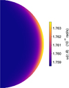Fig. 1 Meridional cross sections of the differential rotation profile Eq. (9) with A = 0.003 and D = 3000 km.

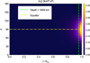Fig. 2 Difference in the centrifugal potential between the differential rotation case (A = 0.003, D = 3000 km) and the rigid rotation case.

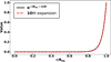Fig. 3 Comparison of the original exponential function with its tenth-order expansion for a given depth of D = 3000 km.

3 Rotating n = 1 polytrope for Jupiter

As a foundational test case, we applied the method described in the previous section to model rotating planets with an n = 1 polytropic structure. This allowed us to intuitively analyze the influence of differential rotation without considering the uncertainties inherent in the equation of state (EOS) and internal structures. Following Ni (2019); Nettelmann et al. (2021), we address the rotating n = 1 polytropic model. The radial coordinate was defined in terms of the mean radius R_m, which was adjusted iteratively to match the observed equatorial radius R_eq. The computational grid used N = 10 000 points in the radial direction, where N/2 were uniformly spaced over 0.85–1 R_m and the other half was evenly distributed in 0–0.85 R_m. For comparison, the parameter settings remained the same as in Wisdom & Hubbard (2016): $q={\omega }^2{R}_{\mathrm{e}\mathrm{q}}^3/GM=0.089195487$, R_eq = 71 492 km and GM = 126686536.1 km³/s². The parameter ω₀ in the differential rotation profile Eq. (9) was fixed to the value $\omega =\sqrt{GMq/R_{\text{eq}}^3}$, while the amplitude parameter A was varied to characterize the different profiles.

Table 1 presents the resulting mean radius $R_{\mathrm{m}}^{\mathrm{f}\mathrm{i}\mathrm{t}}$ and the calculated gravitational harmonics for the case of rigid rotation and various cases of differential rotation. As additional information, the gravitational harmonics derived by the Bessel function (Wisdom & Hubbard 2016) are also shown for the case of rigid rotation. First, our results for rigid rotation show excellent agreement with those of Wisdom & Hubbard (2016). This demonstrates that the TOF5 implementation is sufficiently reliable for a subsequent discussion of differential rotation. Various cases of differential rotation are defined by the intensity A in Eq. (9). Cases 1–6 exhibit the intensity from 0.0005 to 0.010. Given a fixed equatorial radius, a smaller mean radius corresponds to a flatter planetary shape. The results for Cases 1–6 show evident variations in the mean radius $R_{\mathrm{m}}^{\mathrm{f}\mathrm{i}\mathrm{t}}$, highlighting the influence of differential rotation on Jupiter’s shape. The $R_{\mathrm{m}}^{\mathrm{f}\mathrm{i}\mathrm{t}}$ values are systematically lower than in the case of rigid rotation, and this discrepancy increases with increasing rotation intensity, culminating in a deviation of approximately 26 km for Case 6. This trend demonstrates that the intensity of differential rotation induces additional flattening in Jupiter’s shape. The absolute values of the calculated gravitational harmonics exhibit a clear increasing trend with the intensity of differential rotation. As illustrated in Figure 4, this trend is evident in Cases 1 to 6 compared to the case of rigid rotation. Furthermore, the higher-order harmonics have a greater sensitivity to the intensity than their lower-order counterparts. This can be easily understood, since the higher-order gravitational harmonics are more sensitive to the outermost part of the planet (Hubbard 1999; Guillot 2005).

4 Four-layer interior models of Jupiter

4.1 Four-layer structure models and EOSs

The four-layer interior model used in this work is entirely based on our previous work (Ni 2019). For completeness, we provide a brief overview of its key features below. The four distinct layers are defined as follows: (1) a homogeneous molecular hydrogen atmosphere with a depleted helium abundance; (2) a metallic hydrogen envelope enriched in helium; (3) a dilute core region composed of metallic hydrogen, helium, and heavy elements; and (4) a compact isothermal central core composed primarily of rocky material. The numbering of the layers is given in increasing order from the outermost layer to the innermost one. Throughout the text, the corresponding indices are used to denote these different layers. Layers 1 and 2 are separated by the molecular-to-metallic transition of hydrogen. This boundary is defined by a specific transition pressure P_1–2 and is characterized by a corresponding temperature jump ΔT_1–2. For this analysis, the transition pressure P_1–2 was fixed at 2 Mbar and the temperature jump ΔT_1–2 set to 500 K. The interface between Layers 2 and 3 was defined by the pressure P_dil, which was allowed to vary uniformly between 6 and 26 Mbar. Y_i and Z_i represent the mass fractions of helium and heavy element for Layer i, respectively. The heavy elements in Layer 3 consist of both ice and rocks, accounting for the rocks dissolved from the central core. Consequently, we introduced the rock mass fraction in heavy elements, f_rock, to parameterize the heavy elements of this layer, and adopted a value of 0.45 for this work. The helium abundance Y₁ in Layer 1 is constrained by Galileo observations Y₁/(1 − Z₁) = 0.238 ± 0.005 (Von Zahn et al. 1998). Helium abundances in Layers 2 and 3 are constrained by the requirement that the mean helium mass fraction in Jupiter must match its value in the proto-solar nebula Y_proto/(1 − Z_proto) = 0.277 ± 0.006 (Serenelli & Basu 2010). The outer boundary condition was set as T = 165 ± 5 K at 1 bar, based on measurements from the Voyager and Galileo missions (Lindal et al. 1981).

The equations of state (EOSs) are important inputs for interior modeling (Li et al. 2021; Gao et al. 2022; Howard & Guillot 2023; Sur et al. 2024). In this work, we adopted the ab initio EOS CMS-19 (Chabrier et al. 2019) for hydrogen and helium. For heavy elements, the EOS of dry sand in SESAME was used for rocks and the AQUA-EOS of H₂O for ices (Haldemann et al. 2020). For a system composed of hydrogen, helium, and heavy elements, the density and entropy of the mixture can be obtained from the EOS for pure species using the additive volume rule.

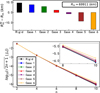Fig. 4 Results for the rotating n = 1 polytrope of Jupiter: calculated mean radii $R_{\mathrm{m}}^{\mathrm{f}\mathrm{i}\mathrm{t}}$ and even gravitational harmonics for rigid rotation and six differential rotation scenarios (Cases 1–6). For the cases of differential rotation, the intensity parameter A ranges from 0.0005 to 0.010.

4.2 Calculated equatorial radius and even gravity harmonics

To quantify the effect of differential rotation on the four-layer structure, we focused on two cases of differential rotation (Diff-3 and Diff-5) and compared them with the rigid-rotation baseline. The two cases differ in their intensity parameter: A = 0.003 for Diff-3 and A = 0.005 for Diff-5. The maximum wind speeds in the equatorial region corresponding to different intensities can be found in Table 1. Following Ni (2019), we considered a wide range of dilute core configurations by varying its size and compositions (P_dil, Y₃, and Z₃) for each case. In order to reproduce Jupiter’s equatorial radius and even low-order gravitational harmonics J₂, J₄, and J₆, the abundances of heavy elements Z₁, Z₂, as well as the compact core mass M_core, were treated as free parameters in our model to explore the possible solutions for Jupiter’s interior. Optimization of observational constraints was achieved by minimizing the following objective function (Saumon & Guillot 2004): $${\chi }^2(Z_1,Z_2,M_{\text{core\hspace{0.17em}}})=\frac{1}{4}[{\left(\frac{R_{\mathrm{e}\mathrm{q}}^{\mathrm{c}\mathrm{a}\mathrm{l}}-R_{\mathrm{e}\mathrm{q}}^{\mathrm{o}\mathrm{b}\mathrm{s}}}{{\sigma }_{R_{\mathrm{e}\mathrm{q}}}}\right)}^2+\sum _{i=1}^3{\left(\frac{J_{2i}^{\mathrm{c}\mathrm{a}\mathrm{l}}-J_{2i}^{\mathrm{s}\mathrm{t}\mathrm{a}\mathrm{t}\mathrm{i}\mathrm{c}}}{{\sigma }_{J_{2i}}}\right)}^2],$$(13)

where σ_n represents the observational uncertainties for different quantities. Table 2 shows the updated measurements of Jupiter’s gravitational field (Durante et al. 2020) and the dynamic contributions from zonal flows (Miguel et al. 2022). Jupiter’s static gravitational harmonics are calculated by subtracting the flow-induced $\mathrm{\Delta }{J}_{2i}^{\text{dyn.}}$ from Juno’s observed $J_{2i}^{\text{Juno}}$ values, giving $J_{2i}^{\text{static}}=J_{2i}^{\text{Juno}}-\mathrm{\Delta }{J}_{2i}^{\text{dyn.}}$.

In view of the dynamical uncertainties in zonal flows, we allowed the model solutions to deviate from the measured values within ~30σ, corresponding to χ² ≤ 10³. Nonetheless, the broad solution space resulted in conspicuous mismatches between certain solutions and observed values. Consequently, we further filtered out solutions with χ² > 10 for subsequent analysis. In all, 359 solutions for rigid rotation, 301 solutions for Diff-3, and 267 solutions for Diff-5 were obtained.

Figure 5 shows the distribution of the calculated equatorial radius ($R_{\text{eq}}^{\text{cal}}$) for all model solutions. The results are tightly clustered around Jupiter’s observed equatorial radius $R_{\text{eq}}^{\text{obs}}$, well within the observational uncertainty. The $R_{\text{eq}}^{\text{cal}}$ values show a slight increase with the intensity of differential rotation, indicating more flattening of the planetary shape. This trend is consistent with our finding for the rotating n = 1 polytrope. Figure 6 shows the resulting gravitational harmonics on the J_i–J_i+2 planes for the three cases, compared to the Juno measured static harmonics $J_{2i}^{\text{static}}$ with 3 σ uncertainties. The lower-order harmonics J₂ and J₄ are well reproduced by numerous model solutions. In contrast, the results of the three cases diverge for the higher-degree harmonics (J₆–J₁₀). Solutions that incorporate differential rotation generally yield larger absolute values for J₆–J₁₀, and this trend becomes more pronounced with increasing the intensity of differential rotation. This behavior is also consistent with our finding shown in Sect. 3.

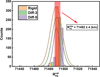Fig. 5 Distribution of the calculated equatorial radii ($R_{\text{eq}}^{\text{cal}}$) for three cases: rigid rotation (Rigid) and two differential rotation scenarios (Diff-3 and Diff-5). The Diff-3 and Diff-5 cases differ in intensity, with A = 0.003 for Diff-3 and A = 0.005 for Diff-5.

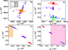Fig. 6 Jupiter’s even gravitational harmonics (J2–J10) from three sets of interior models: rigid rotation (Rigid, blue points) and differential rotation (Diff-3, purple squares; Diff-5, red stars). Shade regions represent Juno’s static gravitational harmonics $J_{2i}^{\text{static}}$ with 3 σ uncertainties.

4.3 Jupiter’s heavy element abundance and distribution

The distribution of heavy elements in Jupiter’s interior provides important information on its formation and evolution. In our four-layer structure model, the heavy-element mass fractions in Layers 1 and 2 (Z₁ and Z₂), and the mass of the compact rocky core (M_core) are adjusted to match Jupiter’s equatorial radius and even low-order gravitational harmonics, and various dilute core configurations are considered by varying its size and compositions (P_dil, Y₃, and Z₃). Figures 7 and 8 illustrate the heavy-element mass fractions in different layers for rigid rotation (Rigid) and two differential rotation cases (Diff-3 and Diff-5). Figure 7a shows the heavy-element mass fraction Z₁ in Layer 1 as a function of the mass fraction Z₂ in Layer 2. For rigid rotation, the resulting Z₁ values fall mostly within the range of 0.02–0.04, and, furthermore, nearly half of the solutions allow Z₁ > Z₂. When differential rotation is taken into account, the resulting Z₁ values are generally reduced with increasing intensity. For the Diff-5 case, the Z₁ values range from 0.005 to 0.015. Figure 7b displays the difference in the heavy-element mass fraction (ΔZ₂₁ = Z₂ − Z₁). For rigid rotation, most model solutions yield ΔZ₂₁ < 0, consistent with the results shown in Figure 7a. In contrast, both differential rotation cases prefer solutions with ΔZ₂₁ > 0, suggesting a heavy-element enrichment in the metallic envelope. Figure 8a shows the heavy-element mass fraction Z₁ in Layer 1 as a function of the mass fraction Z₃ in Layer 3. The dilute core region has a significantly higher heavy-element abundance for all rotation cases. Figure 8b displays the difference in the heavy-element mass fraction (ΔZ₃₁ = Z₃ − Z₁). As the intensity of differential rotation increases, model solutions allow larger ΔZ₃₁ values, indicating greater heavy-element enrichment in the dilute core. With these in mind, differential rotation enhances the heavy-element abundances in both the metallic envelope (Layer 2) and the dilute core region (Layer 3), but reduces that in the molecular envelope (Layer 1). This effect becomes more pronounced with increasing rotation intensity.

In the four-layer structure model, Jupiter’s core mass ($M_{\mathrm{Z}}^{\text{core}}$) is defined as the combination of the compact core mass (M_core) and the heavy elements within the dilute core (M_Z3), $M_{\mathrm{Z}}^{\text{core}}=M_{\text{core}}+M_{{\mathrm{Z}}_3}$. Correspondingly, the heavy-element mass in the envelopes ($M_{\mathrm{Z}}^{\text{env}}$) is the sum of the masses in the molecular and metallic layers, $M_{\mathrm{Z}}^{\text{env}}=M_{{\mathrm{Z}}_1}+M_{{\mathrm{Z}}_2}$. The total heavy-element mass of Jupiter ($M_Z^{\text{total}}$) can be calculated by adding these two components, $M_Z^{\text{total}}=M_{\mathrm{Z}}^{\text{core}}+M_{\mathrm{Z}}^{\text{env}}$. Figure 9 illustrates the total heavy-element mass $M_Z^{\text{total}}$ versus the heavy-element mass in the core $M_{\mathrm{Z}}^{\text{core}}$. Clearly, the total heavy-element mass increases from the rigid rotation case to the Diff-3 and Diff-5 cases. The Diff5 case yields the total heavy-element mass $M_Z^{\text{total}}$ from 14.5 to 16.0 M_⊕, while the rigid-rotation case from 11.5 to 14.0 M_⊕. Also, the Diff-3 and Diff-5 cases allow for more heavy elements in the core with respect to rigid rotation. It is well known that the heavy-element masses in different layers are strongly correlated under the constraints of Jupiter’s shape and gravity field. In order to discern the distribution of heavy elements, we compare the heavy-element masses in different layers for these three cases. Figure 10a displays the heavy-element mass in the molecular hydrogen atmosphere (M_Z1) versus that of the compact rocky core (M_core). In all three cases, one can see that the allowed heavy-element amount M_Z1 shows a clear decreasing tendency with increasing compact core mass M_core. The model solutions without central compact cores exhibit a greater variation in M_Z1, up to roughly 1.0 M_⊕.

Moreover, the model solutions for differential rotation tend to yield a lower M_Z1 in the molecular atmosphere and a smaller compact core M_core. With increasing rotation intensity, the heavy-element mass in the outer envelope decreases from approximately 1.0–2.0 M_⊕ to 0.3–0.8 M_⊕, and the compact core mass shows smaller variations with a maximum M_core value of approximately 5.6–2.8 M_⊕. Figure 10b presents the combined heavy-element mass (M_Z2 + M_Z3) in both the metallic envelope and the dilute core region as a function of the compact core (M_core). The model solutions for differential rotation are confined to a narrow region of available parameter space, corresponding to the higher enrichment in Layers 2 and 3 but to the smaller variations of the compact core mass. When we compare Figures 9 and 10, it is found that the increase in the total heavy-element mass $M_{\mathrm{Z}}^{\text{total}}$ caused by differential rotation is essentially contributed by the enrichment in Layers 2 and 3 while the large variation in $M_{\mathrm{Z}}^{\text{core}}$ stems from the enrichment in Layer 3. Differential rotation appears to enrich the heavy elements in Jupiter’s deep interior, maintaining the dilute core.

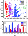Fig. 7 Heavy-element mass fractions in the molecular and metallic envelopes for three sets of interior models: rigid rotation (Rigid, blue points) and differential rotation (Diff-3, purple squares; Diff-5, red stars). (a) Z1 in the molecular envelope versus Z2 in the metallic envelope. (b) Histogram of the abundance difference (ΔZ21 = Z2 − Z1).

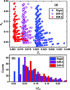Fig. 8 Same as in Figure 7, but showing the heavy-element mass fractions in the molecular envelope (Z1) and the dilute core region (Z3) (ΔZ31 = Z3 − Z1).

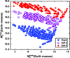Fig. 9 Heavy-element mass in the core including the dilute core region $M_{\mathrm{Z}}^{\text{core}}$ ($M_{\mathrm{Z}}^{\text{core}}=M_{\text{core}}+M_{{\mathrm{Z}}_3}$) as a function of the total heavy-element mass $M_Z^{\text{total}}$ in Jupiter for three sets of interior models: rigid rotation (Rigid, blue points) and differential rotation (Diff-3, purple squares; Diff-5, red stars).

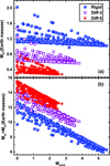Fig. 10 Distribution of heavy elements in the different layers of Jupiter for three sets of interior models: rigid rotation (Rigid, blue points) and differential rotation (Diff-3, purple squares; Diff-5, red stars). (a) The heavy-element mass in the molecular atmosphere (MZ1) is plotted as a function of that in the compact rocky core (Mcore). (b) The combined heavy-element mass (MZ2 + MZ3) in both the metallic envelope and the dilute core region is plotted as a function of that in the compact rocky core (Mcore).

5 Discussion

Jupiter’s heavy-element content provides an important constraint on planet formation models. However, because it cannot be directly measured, it is often inferred by combining the Juno gravity data with interior structure models. The inferred value is consequently sensitive to various factors and assumptions within interior models, such as the EOS (Militzer et al. 2008; Militzer & Hubbard 2013; Miguel et al. 2022), adopted structural model (Nettelmann et al. 2021; Militzer & Hubbard 2024), composition of heavy elements (Ni 2019; Militzer & Hubbard 2024), and atmospheric structure with its properties (Galanti et al. 2019; Kong et al. 2018; Gupta et al. 2022). Many studies have been devoted to exploring the uncertainties in modeling Jupiter’s interior. Here we discuss the effect induced by differential rotation in relation to the other effects.

Jupiter’s total heavy-element mass is primarily affected by the uncertainties in the EOS, which are far greater than that of differential rotation. We only compare the effect of differential rotation with other minor sources of uncertainty. Ni (2019) explored the uncertainty of the composition of heavy elements within the four-layer structure model by varying the rock mass fraction of heavy elements f_rock. A higher rock fraction in the dilute core region is found to yield a lower total heavy-element mass $M_Z^{\text{total}}$, which is independent of the adopted EOS. Using a pure ice composition (f_rock = 0) as a baseline, increasing f_rock to 0.45 reduces $M_Z^{\text{total}}$ by ~2 M_⊕. As shown in Figure 9, the increase in $M_Z^{\text{total}}$ from rigid rotation to the Diff-5 case is approximately 2.5 M_⊕. Thus, the effect of differential rotation is comparable to that of varying the rock fraction of heavy elements.

Helium rain is expected to occur in Jupiter’s interior owing to helium immiscibility in metallic hydrogen. It creates a thin helium gradient between the outer molecular and inner metallic hydrogen envelopes, suppressing large-scale convection. This results in a superadiabatic temperature gradient and a discontinuity in entropy. Modern interior models are required to incorporate this nonadiabatic layer to accurately explain Jupiter’s observed helium depletion and gravity field. The temperature or entropy jump between the molecular and metallic envelopes is often introduced to account for the nonadiabatic effect (Guillot et al. 2018; Ni 2019, 2020b; Miguel et al. 2022; Militzer et al. 2022). Using the dilute-core model with various EOSs, Miguel et al. (2022) determined the posterior distribution of this temperature jump from Markov chain Monte Carlo calculations, yielding a range of 0–500 K. Ni (2019) explored the nonadiabatic effect on Jupiter’s interior by varying the temperature jump ΔT_1–2. It is found that increasing ΔT_1–2, corresponding to stronger nonadiabatic effects, allows for more heavy elements in Jupiter’s interior, with the heavy-element enrichment in both the core and envelope regions. This can be easily understood, since a hotter deep interior has a lower density and the heavy-element amount must be enriched to match the available constraints. As ΔT_1–2 increases from approximately 200–600 K, the total heavy-element mass $M_Z^{\text{total}}$ increases by ~2 M_⊕. By contrast, the increase in $M_Z^{\text{total}}$ from rigid rotation to the Diff-5 case is approximately 2.5 M_⊕, as shown in Figure 9. This suggests that these two effects are comparable in magnitude.

Next, we consider the uncertainty associated with the transition pressure P_1–2, which was previously explored by Nettelmann et al. (2012) and Miguel et al. (2016). Gravitational harmonics are mainly determined by the external levels of a planet, and higher-order ones are increasingly sensitive to the outermost part of a planet (Guillot 2005; Nettelmann et al. 2021). As the pressure P_1–2 increases from 1 to 4 Mbar, the metallic envelope contracts inward, which decreases the calculated gravitational harmonics, particularly for higher-order ones. To compensate for this decrease and match the observed static harmonics, the atmospheric heavy-element amount Z₁ is generally increased and the core mass is decreased. As illustrated in Figure 3 of Nettelmann et al. (2012), an increase in P_1–2 from 1 to 4 Mbar enhances Z₁ by approximately 0.020. This change is comparable to the effect of differential rotation, which reduces atmospheric metallicity Z₁ by roughly 0.020 from rigid rotation to the Diff-5 case, as shown in Figure 7a. Besides, an increase in P_1–2 from 1 to 4 Mbar also decreases the core mass by 2–3 M_⊕, as demonstrated in Figure 3 of Nettelmann et al. (2012) and in Figure 11 of Miguel et al. (2016). This decrease is close to the change in M_core from the rigid rotation to the Diff-5 case, as shown in Figure 10. As expected, the net effect of P_1–2 on the total heavy-element mass $M_Z^{\text{total}}$ is relatively small, because the decrease in the core mass is largely balanced by the increase of heavy elements in the envelope. This is similar to that of differential rotation, where the decrease in heavy elements in the compact core and the outer molecular envelope is compensated by the increase in the metallic envelope and the dilute core region, as shown in Figure 10.

Nettelmann et al. (2021) combined the seventh-order TOF with the four-layer interior model to infer Jupiter’s interior using the CMS-19 H/He EOS. Their model solutions that fit J₂ and J₄ yielded negative Z₁ values between −0.005 and −0.020, which are inconsistent with the Galileo entry probe measurement. To resolve this discrepancy, two scenarios have been proposed. One is to reduce the density in part of the molecular envelope by perturbing the H/He adiabat in view of possible uncertainties in the H/He EOS (Fortney 2007). This was subsequently confirmed by Militzer et al. (2022), who showed that increasing the density deficit in the 10–100 GPa range allows a higher atmospheric metallicity. The other scenario is that Jupiter’s atmosphere may not be well mixed, implying that the Galileo entry probe in a hot spot may not be representative of Jupiter’s global atmosphere. Nettelmann et al. (2021) found that atmospheric metallicity can reach 1 × solar if the surface temperature at the 1 bar level is enhanced by ~14 K from the Galileo entry probe. This conclusion is supported by Miguel et al. (2022) in their three-layer model and dilute-core model. Furthermore, a reassessment of Voyager’s radio occultation data by Gupta et al. (2022) suggested an increase of ~4 K in the 1 bar temperature and revealed a latitude-dependent thermal structure. As demonstrated in Figure 7a, the static effect of differential rotation reduces atmospheric metallicity Z₁. Consequently, to achieve the same atmospheric metallicity, a more pronounced adjustment is required in the interior models: either a larger density deficit in part of the molecular envelope or a higher 1 bar temperature. In other words, the density deficit appears in a shallower region of the molecular envelope or with a larger intensity, or Jupiter’s atmosphere is warmer than previously estimated (Nettelmann et al. 2021; Miguel et al. 2022).

6 Conclusions

The Juno spacecraft has measured Jupiter’s gravitational field to high precision, making the contribution of its zonal flows to the gravity field non-negligible. The dynamic contribution to the gravity field, evaluated from density perturbations induced by zonal winds, has been extensively studied (Kaspi et al. 2020; Kong et al. 2018; Cao et al. 2023). Semi-independent modeling of atmospheric dynamics and interior structure offers a powerful approach to inversion using high-precision gravity data. This method accommodates realistic wind profiles but, as noted by Fortney et al. (2023), neglects how differential rotation distorts the planet’s shape (i.e., the centrifugal deformation of its equipotential surfaces). In this work, we define this influence as the static effect of differential rotation and explicitly incorporate it into our calculation of static gravitational harmonics $J_{2n}^{\text{static}}$. To preliminarily quantify the static effects, we extended the traditional TOF5 by incorporating differential rotation into the calculation of centrifugal potentials. Using this improved framework, we investigated Jupiter’s shape, gravity field, and interior structure, and compared the results with those derived under the assumption of rigid rotation.

We first applied the improved TOF5 to the rotating n = 1 polytropic model under various assumed profiles of differential rotation. Overall, differential rotation yields a more oblate planetary shape with respect to rigid rotation, and the absolute values of even harmonics J_2n increase with increasing intensity of differential rotation, with higher-order harmonics exhibiting a stronger response. We then combined the improved TOF5 with our four-layer structure model (Ni 2019) to infer Jupiter’s interior, adopting the CMS-19 H/He EOS (Chabrier et al. 2019). The static effect of differential rotation on Jupiter’s interior was derived by comparing the calculated J_2n, which includes the centrifugal corrections from differential rotation, with the observed J_2n where the dynamic contribution has been removed. Incorporating differential rotation yields larger absolute values for gravitational harmonics, particularly higher-order ones J₆, J₈, and J₁₀. Consequently, a lower atmospheric metallicity (Z₁) is required to fit the Juno gravity field data. We also find that differential rotation allows for more heavy elements in Jupiter’s interior. The total heavy-element mass spans 11.5–14.0 M_⊕ for rigid rotation, but increases to a range of 14.5–16.0 M_⊕ for Diff-5 differential rotation. More specifically, heavy-element enrichment is primarily concentrated in the metallic envelope and the dilute core region, amounting to an increase of approximately 2–4 M_⊕ for the Diff-5 case, as shown in Figure 10b. Conversely, the mass of the compact core and the heavy-element mass in the molecular atmosphere are reduced. It seems that differential rotation enriches the heavy elements in Jupiter’s deep interior, primarily supporting the maintenance of its dilute core. Since differential rotation reduces atmospheric metallicity, reproducing Galileo’s atmospheric metallicity would require either a density deficit at shallower depths or of greater magnitude in the molecular envelope or a warmer atmospheric temperature than previously estimated (Nettelmann et al. 2021; Militzer et al. 2022; Miguel et al. 2022). The influence of differential rotation on Jupiter’s heavy-element distribution is comparable in magnitude to the other model uncertainties, such as the composition of heavy elements, the presence of a nonadiabatic layer, and the transition pressure between the molecular and metallic layers. Therefore, future interior models should incorporate the aforementioned static effects of differential rotation to achieve a more complete and accurate understanding of Jupiter’s structure.

Acknowledgements

This work is supported by the National Natural Science Foundation of China (Grant Nos. 42578010, T2495234), the Pre-Research Projects on Civil Aerospace Technologies of China National Space Administration (Grant No. D010303), and the Science and Technology Development Fund, Macau SAR (File No. 0139/2024/RIA2).

References

Appendix A Expansion of the exponential term using Chebyshev polynomials

The exponential term exp [−(R_eq − r)/D] in Eq. (10) is a function of the radial distance r, and its domain spans from zero to R_eq. However, the domain of the independent variable does not align with the domain defined for the Chebyshev polynomial. Therefore, the first step in the expansion requires mapping the independent variable to the domain of the Chebyshev polynomials. So we define a dimensionless variable as x = 2r/R_eq − 1 and rewritten the exponential term as $$f(x)=\exp [-\frac{(1-x)}{2d}],x\in [-1,1],$$(A.1)

where d is a dimensionless variable defined as d = D/R_eq. The function f(x) is then expanded in a series of Chebyshev polynomials, $$f(x)\approx \sum _{n=0}^{10}{B}_n{T}_n(x),x\in [-1,1],$$(A.2)

where B_n and T_n are the coefficients and polynomials corresponding to the Chebyshev expansion, respectively. Due to the orthogonality of Chebyshev polynomials, the coefficients B_n can be calculated via the following integration, $$B_n=\frac{2-{\delta }_{n0}}{\pi }{\int }_{-1}^1\frac{f(x)T_n(x)}{\sqrt{1-x^2}}dx,$$(A.3)

where δ_n0 is the Kronecker delta. Next, we perform an inverse transformation to express x in terms of the radial coordinate r. We introduce the dimensionless radial parameter β ≡ r/R_eq. After combining like terms, the original exponential function can be approximated as: $$\exp [-\frac{(R_{eq}-r)}{D}]\approx \sum _{n=0}^{10}{C}_n{\beta }^n.$$(A.4)

For the tenth-order expansion, the combined coefficients C_n are derived from the Chebyshev coefficients B_n through the following relationship: $$\begin{array}{rl}{C}_0=& B_0-B_1+B_2-B_3+B_4-B_5+B_6-B_7+B_8-B_9+B_{10},\\ C_1=& 2B_1-8B_2+18B_3-32B_4+50B_5-72B_6+98B_7\\ & -128B_8+162B_9-200B_{10},\\ C_2=& 8B_2-48B_3+160B_4-400B_5+840B_6-1568B_7\\ & +2688B_8-4320B_9+6600B_{10},\\ C_3=& 32B_3-256B_4+1120B_5-3584B_6+9408B_7-21504B_8\\ & +44352B_9-84480B_{10},\\ C_4=& 128B_4-1280B_5+6912B_6-26880B_7+84480B_8\\ & -228096B_9+549120B_{10},\\ C_5=& 512B_5-6144B_6+39424B_7-180224B_8+658944B_9\\ & -2050048B_{10},\\ C_6=& 2048B_6-28672B_7+212992B_8-1118208B_9\\ & +4659200B_{10},\\ C_7=& 8192B_7-131072B_8+1105920B_9-6553600B_{10},\\ C_8=& 32768B_8-589824B_9+5570560B_{10},\\ C_9=& 131072B_9-2621440B_{10},\\ C_{10}=& 524288B_{10}.\end{array}$$(A.5)

It is important to note that for relatively shallower depths (e.g., 1000 km), higher-order expansions are necessary to accurately capture the rapid decay of the exponential function, and the relationship in Eq. (A.5) is no longer applicable.

Appendix B Expansion of the centrifugal potential

To incorporate the centrifugal potential for differential rotation into the TOF5 framework, it must be expanded in a series of Legendre polynomials. Consequently, each term in Eq. (12) requires expansion via Legendre polynomials. The first term, which is identical to the rigid rotation case, has already been addressed in Sect. 2.1. Here, we focus on the perturbation. Using the first term of the perturbation as an example, we expand it in a series of Legendre polynomials: $$Q_0^p=A{C}_0{\omega }_0^2[l(1+\mathrm{\Sigma }){]}^2{\sin }^4\theta =A{C}_0{\omega }_0^2{l}^2\sum _{k=0}^5{D}_{2k}^0{P}_{2k}(\cos \theta ),$$(B.1)

where A and C₀ are constants, and $D_{2k}^0$ are the expansion coefficients for the even-order Legendre polynomials. The coefficients $D_{2k}^0$ can be calculated by $$D_{2k}^0=\frac{4k+1}{2}{\int }_{-1}^1(1+\mathrm{\Sigma }{)}^2{\sin }^4\theta P_{2k}(\cos \theta )d\cos \theta .$$(B.2)

The sin⁴ θ can be rewritten using Legendre polynomials as $${\sin }^4\theta =\frac{8}{35}{P}_4(\cos \theta )-\frac{16}{21}{P}_2(\cos \theta )+\frac{8}{15}.$$(B.3)

In the TOF5, the Σ in the level surface is $$\mathrm{\Sigma }=\sum _0^5{s}_{2k}(l)P_{2k}(\cos \theta ),$$(B.4)

with $$s_0=-\frac{1}{5}{s}_2^2-\frac{2}{105}{s}_2^3-\frac{1}{9}{s}_4^2-\frac{2}{35}{s}_2^2{s}_4-\frac{20}{693}{s}_2{s}_4^2-\frac{2}{525}{s}_2^5.$$(B.5)

Next, we substitute Eqs. (B.3–B.5) into Eq. (B.2) and remove all terms contributing nothing to the integral in Eq. (B.2). The details on this procedure can be found in Appendix A.5 of Nettelmann et al. (2021). Here we give the final expressions of $D_{2k}^0$, $$\begin{array}{rl}{D}_0^0=& \frac{1496}{55125}{s}_2^4+\frac{64}{1575}{s}_2^3-\frac{16}{225}{s}_2^2{s}_4-\frac{24}{175}{s}_2^2-\frac{256}{3465}{s}_2{s}_4\\ & +\frac{16}{1001}{s}_2{s}_6-\frac{32}{105}{s}_2-\frac{10424}{135135}{s}_4^2+\frac{16}{315}{s}_4+\frac{8}{15},\end{array}$$(B.6) $$\begin{array}{rl}{D}_2^0=& -\frac{496}{11025}{s}_2^4-\frac{272}{2205}{s}_2^3+\frac{3904}{24255}{s}_2^2{s}_4+\frac{64}{385}{s}_2^2+\frac{1424}{9009}{s}_2{s}_4\\ & -\frac{96}{1001}{s}_2{s}_6+\frac{16}{21}{s}_2+\frac{3184}{27027}{s}_4^2-\frac{256}{693}{s}_4+\frac{80}{1001}{s}_6-\frac{16}{21},\end{array}$$(B.7) $$\begin{array}{rl}{D}_4^0=& \frac{4408}{202125}{s}_2^4+\frac{5024}{40425}{s}_2^3-\frac{30672}{175175}{s}_2^2{s}_4+\frac{1272}{25025}{s}_2^2\\ & -\frac{928}{5005}{s}_2{s}_4+\frac{2864}{17017}{s}_2{s}_6-\frac{256}{385}{s}_2-\frac{28744}{765765}{s}_4^2\\ & +\frac{3728}{5005}{s}_4-\frac{32}{77}{s}_6+\frac{224}{2431}{s}_8+\frac{8}{35},\end{array}$$(B.8) $$\begin{array}{rl}{D}_6^0=& -\frac{32}{8085}{s}_2^4-\frac{16}{385}{s}_2^3+\frac{416}{3465}{s}_2^2{s}_4-\frac{48}{385}{s}_2^2+\frac{2864}{11781}{s}_2{s}_4\\ & -\frac{13952}{74613}{s}_2{s}_6+\frac{16}{77}{s}_2-\frac{544}{13167}{s}_4^2-\frac{416}{693}{s}_4+\frac{2096}{2805}{s}_6\\ & -\frac{23296}{53295}{s}_8.\end{array}$$(B.9) $$\begin{array}{rl}{D}_8^0=& -\frac{224}{6435}{s}_2^2{s}_4+\frac{32}{715}{s}_2^2-\frac{5248}{24453}{s}_2{s}_4+\frac{1888}{8151}{s}_2{s}_6\\ & +\frac{2416}{24453}{s}_4^2+\frac{224}{1287}{s}_4-\frac{1792}{3135}{s}_6+\frac{19408}{25935}{s}_8,\end{array}$$(B.10) $$\begin{array}{rl}{D}_{10}^0=& \frac{3360}{46189}{s}_2{s}_4-\frac{211008}{1062347}{s}_2{s}_6-\frac{5600}{62491}{s}_4^2+\frac{672}{4199}{s}_6\\ & -\frac{4128}{7429}{s}_8.\end{array}$$(B.11)

The same method is used for the other terms of the perturbation, $Q_n^p(n=1-10)$, yielding the corresponding expansion coefficients $D_{2k}^n$. The perturbation is finally expressed as $$Q^p(l,\theta )=G\overline{\rho }{l}^{2}Am\sum _{k=0}^5\sum _{n=0}^{10}{C}_n{\beta }^n{D}_{2k}^n(l)P_{2k}(\cos \theta ),$$(B.12)

where $m={\omega }_0^3{R}_m^3/GM$ is the dimensionless rotation parameter, as defined in Eq. (7).

All Tables

All Figures

	Fig. 1 Meridional cross sections of the differential rotation profile Eq. (9) with A = 0.003 and D = 3000 km.
In the text

	Fig. 2 Difference in the centrifugal potential between the differential rotation case (A = 0.003, D = 3000 km) and the rigid rotation case.
In the text

	Fig. 3 Comparison of the original exponential function with its tenth-order expansion for a given depth of D = 3000 km.
In the text

	Fig. 4 Results for the rotating n = 1 polytrope of Jupiter: calculated mean radii $R_{\mathrm{m}}^{\mathrm{f}\mathrm{i}\mathrm{t}}$ and even gravitational harmonics for rigid rotation and six differential rotation scenarios (Cases 1–6). For the cases of differential rotation, the intensity parameter A ranges from 0.0005 to 0.010.
In the text

	Fig. 5 Distribution of the calculated equatorial radii ($R_{\text{eq}}^{\text{cal}}$) for three cases: rigid rotation (Rigid) and two differential rotation scenarios (Diff-3 and Diff-5). The Diff-3 and Diff-5 cases differ in intensity, with A = 0.003 for Diff-3 and A = 0.005 for Diff-5.
In the text

	Fig. 6 Jupiter’s even gravitational harmonics (J2–J10) from three sets of interior models: rigid rotation (Rigid, blue points) and differential rotation (Diff-3, purple squares; Diff-5, red stars). Shade regions represent Juno’s static gravitational harmonics $J_{2i}^{\text{static}}$ with 3 σ uncertainties.
In the text

	Fig. 7 Heavy-element mass fractions in the molecular and metallic envelopes for three sets of interior models: rigid rotation (Rigid, blue points) and differential rotation (Diff-3, purple squares; Diff-5, red stars). (a) Z1 in the molecular envelope versus Z2 in the metallic envelope. (b) Histogram of the abundance difference (ΔZ21 = Z2 − Z1).
In the text

	Fig. 8 Same as in Figure 7, but showing the heavy-element mass fractions in the molecular envelope (Z1) and the dilute core region (Z3) (ΔZ31 = Z3 − Z1).
In the text

	Fig. 9 Heavy-element mass in the core including the dilute core region $M_{\mathrm{Z}}^{\text{core}}$ ($M_{\mathrm{Z}}^{\text{core}}=M_{\text{core}}+M_{{\mathrm{Z}}_3}$) as a function of the total heavy-element mass $M_Z^{\text{total}}$ in Jupiter for three sets of interior models: rigid rotation (Rigid, blue points) and differential rotation (Diff-3, purple squares; Diff-5, red stars).
In the text

Fig. 10 Distribution of heavy elements in the different layers of Jupiter for three sets of interior models: rigid rotation (Rigid, blue points) and differential rotation (Diff-3, purple squares; Diff-5, red stars). (a) The heavy-element mass in the molecular atmosphere (MZ1) is plotted as a function of that in the compact rocky core (Mcore). (b) The combined heavy-element mass (MZ2 + MZ3) in both the metallic envelope and the dilute core region is plotted as a function of that in the compact rocky core (Mcore).

In the text

References

- Bolton, S. J., Adriani, A., Adumitroaie, V., et al. 2017, Science, 356, 821 [Google Scholar]
- Cao, H., & Stevenson, D. J. 2017, J. Geophys. Res. Planets, 122, 686 [Google Scholar]
- Cao, H., Bloxham, J., Park, R. S., et al. 2023, ApJ, 959, 78 [Google Scholar]
- Chabrier, G., Mazevet, S., & Soubiran, F. 2019, ApJ, 872, 51 [NASA ADS] [CrossRef] [Google Scholar]
- Debras, F., & Chabrier, G. 2018, A&A, 609, A97 [NASA ADS] [CrossRef] [EDP Sciences] [Google Scholar]
- Demarcus, W. C. 1958, AJ, 63, 2 [Google Scholar]
- Durante, D., Parisi, M., Serra, D., et al. 2020, Geophys. Res. Lett., 47, e2019GL086572 [CrossRef] [Google Scholar]
- Fortney, J. J. 2007, Astrophys. Space Sci., 307, 279 [Google Scholar]
- Fortney, J. J., & Nettelmann, N. 2010, Space Sci. Rev., 152, 423 [CrossRef] [Google Scholar]
- Fortney, J., Militzer, B., Mankovich, C., et al. 2023, arXiv e-prints [arXiv:2304.09215] [Google Scholar]
- Galanti, E., & Kaspi, Y. 2016, ApJ, 820, 91 [NASA ADS] [CrossRef] [Google Scholar]
- Galanti, E., Kaspi, Y., Miguel, Y., et al. 2019, Geophys. Res. Lett., 46, 616 [Google Scholar]
- Gao, H., Liu, C., Shi, J., et al. 2022, Phys. Rev. Lett., 128, 035702 [Google Scholar]
- Guillot, T. 1999, Science, 286, 72 [NASA ADS] [CrossRef] [Google Scholar]
- Guillot, T. 2005, Annu. Rev. Earth Planet. Sci., 33, 493 [Google Scholar]
- Guillot, T., Miguel, Y., Militzer, B., et al. 2018, Nature, 555, 227 [Google Scholar]
- Gupta, P., Atreya, S. K., Steffes, P. G., et al. 2022, Planet. Sci. J., 3, 159 [NASA ADS] [CrossRef] [Google Scholar]
- Haldemann, J., Alibert, Y., Mordasini, C., & Benz, W. 2020, A&A, 643, A105 [NASA ADS] [CrossRef] [EDP Sciences] [Google Scholar]
- Howard, S., & Guillot, T. 2023, A&A, 672, L1 [NASA ADS] [CrossRef] [EDP Sciences] [Google Scholar]
- Hubbard, W. 1968, ApJ, 152, 745 [NASA ADS] [CrossRef] [Google Scholar]
- Hubbard, W. 1969, ApJ, 155, 333 [NASA ADS] [CrossRef] [Google Scholar]
- Hubbard, W. 1999, Icarus, 137, 357 [Google Scholar]
- Hubbard, W. 2013, ApJ, 768, 43 [NASA ADS] [CrossRef] [Google Scholar]
- Iess, L., Folkner, W., Durante, D., et al. 2018, Nature, 555, 220 [NASA ADS] [CrossRef] [Google Scholar]
- Jeffreys, H. 1924, MNRAS, 84, 534 [Google Scholar]
- Kaspi, Y., Galanti, E., Hubbard, W., et al. 2018, Nature, 555, 223 [NASA ADS] [CrossRef] [Google Scholar]
- Kaspi, Y., Galanti, E., Showman, A. P., et al. 2020, Space Sci. Rev., 216, 84 [Google Scholar]
- Kaspi, Y., Galanti, E., Park, R., et al. 2023, Nat. Astron., 7, 1463 [Google Scholar]
- Kong, D., Zhang, K., & Schubert, G. 2016, ApJ, 826, 127 [Google Scholar]
- Kong, D., Zhang, K., Schubert, G., & Anderson, D. J., 2018, Proc. Natl. Acad. Sci. U.S.A., 115, 8499 [Google Scholar]
- Li, G., Li, Z., Chen, Q., et al. 2021, Phys. Rev. Lett., 126, 075701 [Google Scholar]
- Lindal, G. F., Wood, G., Levy, G., et al. 1981, J. Geophys. Res., 86, 8721 [NASA ADS] [CrossRef] [Google Scholar]
- Liu, J., Schneider, T., & Kaspi, Y. 2013, Icarus, 224, 114 [Google Scholar]
- Liu, S., Hori, Y., Müller, S., et al. 2019, Nature, 572, 355 [NASA ADS] [CrossRef] [Google Scholar]
- Low, F. J. 1966, AJ, 71, 391 [NASA ADS] [CrossRef] [Google Scholar]
- Miguel, Y., Guillot, T., & Fayon, L. 2016, A&A, 596, A114 [NASA ADS] [CrossRef] [EDP Sciences] [Google Scholar]
- Miguel, Y., Bazot, M., Guillot, T., et al. 2022, A&A, 662, A18 [NASA ADS] [CrossRef] [EDP Sciences] [Google Scholar]
- Militzer, B., & Hubbard, W. 2013, ApJ, 774, 148 [NASA ADS] [CrossRef] [Google Scholar]
- Militzer, B., & Hubbard, W. 2024, Icarus, 411, 115955 [NASA ADS] [CrossRef] [Google Scholar]
- Militzer, B., Hubbard, W., Vorberger, J., et al. 2008, ApJ, 688, L45 [Google Scholar]
- Militzer, B., Wahl, S., & Hubbard, W. 2019, ApJ, 879, 78 [Google Scholar]
- Militzer, B., Hubbard, W., Wahl, S., et al. 2022, Planet. Sci. J., 3, 185 [NASA ADS] [CrossRef] [Google Scholar]
- Morf, L., Müller, S., & Helled, R. 2024, A&A, 690, A105 [NASA ADS] [CrossRef] [EDP Sciences] [Google Scholar]
- Nettelmann, N. 2020, in AGU Fall Meeting Abstracts, P066-0007 [Google Scholar]
- Nettelmann, N., Becker, A., Holst, B., & Redmer, R. 2012, ApJ, 750, 52 [NASA ADS] [CrossRef] [Google Scholar]
- Nettelmann, N., Movshovitz, N., Ni, D., et al. 2021, Planet. Sci. J., 2, 241 [NASA ADS] [CrossRef] [Google Scholar]
- Neuenschwander, B. A., Helled, R., Movshovitz, N., et al. 2021, ApJ, 910, 38 [NASA ADS] [CrossRef] [Google Scholar]
- Ni, D. 2018, A&A, 613, A32 [NASA ADS] [CrossRef] [EDP Sciences] [Google Scholar]
- Ni, D. 2019, A&A, 632, A76 [NASA ADS] [CrossRef] [EDP Sciences] [Google Scholar]
- Ni, D. 2020a, Earth Planet. Phys., 4, 111 [Google Scholar]
- Ni, D. 2020b, A&A, 639, A10 [NASA ADS] [CrossRef] [EDP Sciences] [Google Scholar]
- Peebles, P. 1964, ApJ, 140, 328 [NASA ADS] [CrossRef] [Google Scholar]
- Porco, C. C., West, R. A., McEwen, A., et al. 2003, Science, 299, 1541 [NASA ADS] [CrossRef] [Google Scholar]
- Russell, C., Yu, Z., & Kivelson, M. 2001, Geophys. Res. Lett., 28, 1911 [Google Scholar]
- Salpeter, E. 1973, ApJ, 181, L83 [Google Scholar]
- Saumon, D., & Guillot, T. 2004, ApJ, 609, 1170 [NASA ADS] [CrossRef] [Google Scholar]
- Serenelli, A. M., & Basu, S. 2010, ApJ, 719, 865 [NASA ADS] [CrossRef] [Google Scholar]
- Smoluchowski, R. 1967, Nature, 215, 691 [NASA ADS] [CrossRef] [Google Scholar]
- Sur, A., Tejada Arevalo, R., Su, Y., & Burrows, A. 2024, ApJS, 274, 34 [Google Scholar]
- Sur, A., Tejada Arevalo, R., Su, Y., & Burrows, A. 2025, ApJ, 980, L5 [Google Scholar]
- Vasavada, A. R., & Showman, A. P. 2005, Rep. Prog. Phys., 68, 1935 [Google Scholar]
- Vazan, A., Helled, R., Kovetz, A., & Podolak, M. 2015, ApJ, 803, 32 [NASA ADS] [CrossRef] [Google Scholar]
- Vazan, A., Helled, R., & Guillot, T. 2018, A&A, 610, L14 [NASA ADS] [CrossRef] [EDP Sciences] [Google Scholar]
- Venturini, J., & Helled, R. 2020, A&A, 634, A31 [NASA ADS] [CrossRef] [EDP Sciences] [Google Scholar]
- Von Zahn, U., Hunten, D., & Lehmacher, G. 1998, J. Geophys. Res. Planets, 103, 22815 [CrossRef] [Google Scholar]
- Wahl, S. M., Hubbard, W., Militzer, B., et al. 2017, Geophys. Res. Lett., 44, 4649 [CrossRef] [Google Scholar]
- Wigner, E., & Huntington, H. B. 1935, J. Chem. Phys., 3, 764 [Google Scholar]
- Wildt, R. 1947, MNRAS, 107, 84 [NASA ADS] [Google Scholar]
- Wisdom, J., & Hubbard, W. 2016, Icarus, 267, 315 [NASA ADS] [CrossRef] [Google Scholar]
- Zharkov, V. N., & Trubitsyn, V. P. 1975, Azh, 52, 599 [Google Scholar]
- Zharkov, V. N., & Trubitsyn, V. P. 1978, Phys. Planet. Interiors [Google Scholar]