© The Authors 2026

1. Introduction

Type II supernovae (SNe) are explosions of red supergiant stars, whose initial zero-age-main-sequence masses are between ∼8 and ∼18 M_⊙ (e.g., Smartt 2015; Van Dyk 2025). Recent observations of Type II SNe have brought a challenge to our understanding of the final evolutionary stages of massive stars. Their early-phase spectra and light curves suggest that a significant fraction of Type II SNe have dense circumstellar material (CSM) in their vicinity (≲10¹⁵ cm; so-called confined CSM), corresponding to mass-loss rates of ∼10⁻⁴ − 1 M_⊙ yr⁻¹ (e.g., Khazov et al. 2016; Yaron et al. 2017; Förster et al. 2018; Boian & Groh 2020; Bruch et al. 2021). However, these extensive mass eruptions cannot be quantitatively explained by currently proposed mechanisms, such as mass eruptions due to stellar instabilities (e.g., Humphreys & Davidson 1994; Langer et al. 1999; Yoon & Cantiello 2010; Arnett & Meakin 2011; Quataert & Shiode 2012; Shiode & Quataert 2014; Smith & Arnett 2014; Woosley & Heger 2015; Quataert et al. 2016; Fuller 2017; Sengupta et al. 2026) or binary interaction (e.g., Chevalier 2012; Soker & Kashi 2013).

Deriving the spatial distribution of the confined CSM is important for clarifying the mass-loss mechanism, which creates it. The early-time polarimetry of the Type II SN 2023ixf suggests that its confined CSM is aspherical and exhibits a continuum polarization of ∼1 % within the first few days (Vasylyev et al. 2023; Singh et al. 2024; Shrestha et al. 2025). The first quantitative demonstration that electron scattering in the confined CSM is the origin of the early-time polarization in SN 2023ixf was presented by Vasylyev et al. (2025). They modeled the polarization using 2D radiative transfer calculations based on an aspherical CSM density distribution, derived by modifying the CSM density geometry in the best-fit 1D nonlocal thermodynamic equilibrium (non-LTE) radiative transfer and radiation-hydrodynamic calculations that reproduce the early-time photometric and spectroscopic properties of SN 2023ixf. They found that the polarization spectrum of SN 2023ixf 2.5 days after the explosion can be quantitatively explained by electron scattering in the aspherical CSM with a pole-to-equator density contrast of ≳3. It should be noted, however, that this modification of the CSM density could alter the expected early-time photometric and spectroscopic properties, implying that the original best-fit parameters for the SN and CSM properties may no longer provide satisfactory fits. Furthermore, it is not clear if the time evolution of the observed early-time polarization in SN 2023ixf can be explained by this scenario with electron scattering in the confined CSM. Dessart et al. (2025) presented a similar attempt to account for the early-time polarization observed in the interacting Type II SN 1998S using electron scattering within its CSM, employing radiative transfer calculations.

In this study, we analytically calculate the time evolution of the polarization signals originating from the confined CSM in Type II SNe. Moreover, we discuss their dependence on various CSM parameters, with the aim of constraining the CSM distribution by applying our calculations to polarimetric observations. In Section 2, we describe our calculation methods for the polarization signals created by the electron scattering processes within the CSM. In Section 3, we provide the results and discuss the dependence of the polarization on the parameters of the confined CSM. In Section 4, we discuss the limitations of our calculations. We conclude the paper with discussions in Section 5.

2. Calculations

In this section, we describe our methodology to calculate the polarization signals that originate from the confined CSM. Figure 1 shows a schematic picture of our calculations. For the CSM, we consider a disk-shaped structure, whose inner and outer edges lie at the surface of the progenitor star (R_p) and at a radius of r_out, respectively, with a half-opening angle of θ_disk. The observer is located on the x–z plane at an angle θ_obs from the z-axis. We assume that the radiation is created only by the interaction between the SN ejecta and the confined CSM, ignoring the radiation from the SN ejecta. This can be realized at early phases of Type II SNe, if they have dense, confined CSM (for the first few weeks; e.g., Ertini et al. 2025). We also assume, for simplicity, that the confined CSM is fully ionized and that electron scattering within the CSM is the only radiation process.

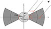Fig. 1. Schematic representation of our calculations. The radiation is generated by the interaction between the SN ejecta the disk-like CSM, with a luminosity of Lsh. A portion of this radiation escapes from the surface of the CSM disk before reaching the photosphere (indicated by the dotted lines in the CSM), with a luminosity of Lsurface, while the remaining radiation escapes from the photosphere, with a luminosity of Lph. The radiation emitted from the photosphere can be polarized due to the last scattering above the photosphere.

First, we calculated the radiation generated by the CSM interaction using the analytical formula from Moriya et al. (2013), based on the assumed SN ejecta and CSM properties. Then, we divided the radiation into two components: the radiation that eventually escapes from the photosphere in the radial direction of the CSM disk and the one that escapes from the photosphere at the surface of the CSM disk (see Figure 1), treating the polarization of these components separately. Once the unshocked CSM became optically thin, we treated all the radiation as escaping from the photosphere in the interaction region.

2.1. SN ejecta and CSM properties

For the SN ejecta, we assume homologous expansion and that the density profile follows the outer part of the double power-law distribution proposed by numerical calculations of SN explosions Matzner & McKee (1999), see also Moriya et al. (2013)):

$$\begin{array}{c}\hfill {\rho }_{\mathrm{ej}}(v_{\mathrm{ej}},t)=\frac{1}{4\pi (n-\delta )}\frac{{[2(5-\delta )(n-5)E_{\mathrm{ej}}]}^{\frac{n-3}{2}}}{{[(3-\delta )(n-3)M_{\mathrm{ej}}]}^{\frac{n-5}{2}}}{t}^{-3}{v}_{\mathrm{ej}}^{-n}.\end{array}$$(1)

Here, v_ej(r, t) (=r/t) is the velocity of the SN ejecta at radius, r, and time, t. We assume that n = 12 and δ = 1, which are typical values for the outer ejecta of a red supergiant progenitor (e.g., Matzner & McKee 1999). Throughout the paper, we also assume the ejecta mass (M_ej) and energy (E_ej) to be 10 M_⊙ and 10⁵¹ erg, respectively, which are typical values for Type IIP SNe (e.g., Martinez et al. 2022).

We assume that the density of the CSM depends solely on the distance from the center of the SN ejecta, and that its radial distribution within the disk follows a power law, ρ_disk(r) = Dr^−s. Instead of the parameter D, we used the total mass of the disk CSM (M_csm) to characterize the CSM density. The total mass of the CSM is related to D as follows:

$$\begin{array}{c}\hfill M_{\mathrm{disk}}={\displaystyle {\int }_{R_{\mathrm{p}}}^{r_{\mathrm{out}}}}4\pi {\omega }_{\mathrm{disk}}{r}^2{\rho }_{\mathrm{disk}}(r)\mathrm{d}r=\frac{4\pi {\omega }_{\mathrm{disk}}D}{3-s}(r_{\mathrm{out}}^{3-s}-R_{\mathrm{p}}^{3-s}),\end{array}$$(2)

where ω_disk = Ω_disk/4π = sin θ_disk, and Ω_disk is the solid angle subtended by the CSM disk covering the SN ejecta. Thus, we get the following equation:

$$\begin{array}{c}\hfill D=\frac{(3-s)M_{\mathrm{disk}}}{4\pi {\omega }_{\mathrm{disk}}(r_{\mathrm{out}}^{3-s}-R_{\mathrm{p}}^{3-s})}.\end{array}$$(3)

In the case of s = 2, we can define the corresponding mass-loss rate to create the disk CSM as follows:

$$\begin{array}{cc}\hfill {\dot{M}}_{\mathrm{disk}}& =\frac{M_{\mathrm{disk}}{v}_{\mathrm{csm}}}{r_{\mathrm{out}}-R_{\mathrm{p}}},\hfill \\ \hfill & \sim 1\times {10}^{-1}\left(\frac{M_{\mathrm{disk}}}{{10}^{-1}[{\mathrm{M}}_{\odot }]}\right)\left(\frac{v_{\mathrm{csm}}}{100[\mathrm{km}{\mathrm{s}}^{-1}]}\right){\left(\frac{r_{\mathrm{out}}}{3\times {10}^{14}[\mathrm{cm}]}\right)}^{-1}\hfill \\ \hfill & [{\mathrm{M}}_{\odot }{\mathrm{yr}}^{-1}].\hfill \end{array}$$(4)

Here, we assume that r_out > > R_p. We also assume that the velocity of the CSM (v_csm) is 100 km s⁻¹, as inferred for SN 2023ixf (Smith et al. 2023), throughout the paper.

2.2. CSM interaction

We calculated the bolometric luminosity created by the interaction between the SN ejecta and CSM disk (L_sh), using the analytical model proposed by Moriya et al. (2013). The time evolution of the location (r_sh(t)) and velocity (v_sh(t)) of the shocked shell can be calculated by solving the equation of motion of the shocked shell, assuming its width is negligible compared to its radius:

$$\begin{array}{cc}\hfill M_{\mathrm{sh}}(t)\frac{\mathrm{d}{v}_{\mathrm{sh}}(t)}{\mathrm{d}t}& =4\pi {\omega }_{\mathrm{disk}}{r}_{\mathrm{sh}}^2(t)[{\rho }_{\mathrm{ej}}(r_{\mathrm{sh}}(t),t){(v_{\mathrm{ej}}(r_{\mathrm{sh}}(t),t)-v_{\mathrm{sh}}(t))}^2\hfill \\ \hfill & -{\rho }_{\mathrm{disk}}(r_{\mathrm{sh}}(t)){(v_{\mathrm{sh}}(t)-v_{\mathrm{csm}})}^2].\hfill \end{array}$$(5)

Here, v_sh(t) is the velocity of the shocked shell at time t, and M_sh(t) is the total mass of the shocked shell at time t, shown as follows:

$$\begin{array}{c}\hfill M_{\mathrm{sh}}(t)={\displaystyle {\int }_{R_{\mathrm{p}}}^{r_{\mathrm{sh}}(t)}}4\pi {\omega }_{\mathrm{disk}}{r}^2{\rho }_{\mathrm{disk}}(r)\mathrm{d}r+{\displaystyle {\int }_{r_{\mathrm{sh}}(t)}^{r_{\mathrm{ej},\max }(t)}}4\pi r^2{\omega }_{\mathrm{disk}}{\rho }_{\mathrm{ej}}(r,t)\mathrm{d}r,\end{array}$$(6)

where r_ej, max(t) = v_ej, maxt and v_ej, max is the original velocity of the outermost layer of the SN ejecta before the CSM interaction. Here, we assume r_sh(t)≫R_p and r_ej, max(t)≫r_sh(t).

Using Eq. (5), we can analytically calculate the time evolution of the shocked shell and its velocity as follows (see Moriya et al. (2013)):

$$\begin{array}{c}\hfill r_{\mathrm{sh}}(t)={\left[\frac{(3-s)(4-s)}{4\pi D(n-4)(n-3)(n-\delta )}\frac{{[2(5-\delta )(n-5)E_{\mathrm{ej}}]}^{(n-3)/2}}{{[(3-\delta )(n-3)M_{\mathrm{ej}}]}^{(n-5)/2}}\right]}^{\frac{1}{n-s}}{t}^{\frac{n-3}{n-s}},\end{array}$$(7)

and

$$\begin{array}{cc}\hfill v_{\mathrm{sh}}(t)& =\frac{n-3}{n-s}{\left[\frac{(3-s)(4-s)}{4\pi D(n-4)(n-3)(n-\delta )}\frac{{[2(5-\delta )(n-5)E_{\mathrm{ej}}]}^{(n-3)/2}}{{[(3-\delta )(n-3)M_{\mathrm{ej}}]}^{(n-5)/2}}\right]}^{\frac{1}{n-s}}\hfill \\ \hfill & t^{-\frac{3-s}{n-s}}.\hfill \end{array}$$(8)

We assume the bolometric luminosity from the shocked shell to be a fraction of the released energy by the shock, as follows:

$$\begin{array}{c}\hfill L_{\mathrm{sh}}(t)=ϵ\frac{\mathrm{d}{E}_{\mathrm{kin}}(t)}{\mathrm{d}t}=2\pi {\omega }_{\mathrm{disk}}ϵ{\rho }_{\mathrm{disk}}(r_{\mathrm{sh}}(t))r_{\mathrm{sh}}^2(t)v_{\mathrm{sh}}^3(t),\end{array}$$(9)

where ϵ represents the conversion efficiency from kinetic energy to radiation, and

$$\begin{array}{c}\hfill \mathrm{d}{E}_{\mathrm{kin}}(t)=4\pi {\omega }_{\mathrm{disk}}{r}_{\mathrm{sh}}^2(t)\left(\frac{1}{2}{\rho }_{\mathrm{disk}}(r_{\mathrm{sh}}(t))v_{\mathrm{sh}}^2(t)\right)\mathrm{d}r.\end{array}$$(10)

We note that choosing the value of ϵ does not affect the calculated polarization degrees. Subsequently, the luminosity from the photosphere and surface of the optically thick region of the disk is simply assumed to be determined by the relative optical depths of the CSM disk along the radial and perpendicular directions (τ_csm, r and τ_csm, h, respectively) without taking the diffusion time into account:

$$\begin{array}{c}\hfill L_{\mathrm{ph}}(t)=\{\begin{array}{c}{L}_{\mathrm{sh}}(t)\times \frac{{\tau }_{\mathrm{csm},\mathrm{h}}(r_{\mathrm{sh}})}{{\tau }_{\mathrm{csm},\mathrm{r}}(r_{\mathrm{sh}})+{\tau }_{\mathrm{csm},\mathrm{h}}(r_{\mathrm{sh}})}({\tau }_{\mathrm{csm},\mathrm{r}}(r_{\mathrm{sh}})\ge 1)\hfill \\ L_{\mathrm{sh}}(t)({\tau }_{\mathrm{csm},\mathrm{r}}(r_{\mathrm{sh}})<1)\hfill \end{array},\end{array}$$(11)

and

$$\begin{array}{c}\hfill L_{\mathrm{surface}}(t)=\{\begin{array}{c}{L}_{\mathrm{sh}}(t)\times \frac{{\tau }_{\mathrm{csm},\mathrm{r}}(r_{\mathrm{sh}})}{{\tau }_{\mathrm{csm},\mathrm{r}}(r_{\mathrm{sh}})+{\tau }_{\mathrm{csm},\mathrm{h}}(r_{\mathrm{sh}})}({\tau }_{\mathrm{csm},\mathrm{r}}(r_{\mathrm{sh}})\ge 1)\hfill \\ 0({\tau }_{\mathrm{csm},\mathrm{r}}(r_{\mathrm{sh}})<1)\hfill \end{array}.\end{array}$$(12)

Here, we simply define the reference optical depths (τ_csm, r and τ_csm, h) as the optical depths along the radial direction and along the inner radius of the CSM disk, respectively, as follows:

$$\begin{array}{cc}\hfill {\tau }_{\mathrm{csm},r}(r)& ={\displaystyle {\int }_r^{r_{\mathrm{out}}}}{\kappa }_{\mathrm{es}}D{r}^{-s}\mathrm{d}r,\hfill \\ \hfill & =\frac{{\kappa }_{\mathrm{es}}D}{s-1}(r^{-(s-1)}-r_{\mathrm{out}}^{-(s-1)}).\hfill \end{array}$$(13)

$$\begin{array}{cc}\hfill {\tau }_{\mathrm{csm},h}(r)& ={\kappa }_{\mathrm{es}}{\rho }_{\mathrm{csm}}(r)r{\theta }_{\mathrm{disk}},\hfill \\ \hfill & ={\kappa }_{\mathrm{es}}D{r}^{-(s-1)}{\theta }_{\mathrm{disk}},\hfill \end{array}$$(14)

and the location of the photosphere is determined by τ_csm, r(r_ph) = 1 when τ_csm, r(r_sh)≥1; otherwise, r_ph = r_sh.

In cases with θ_obs ≦ π/2 − θ_disk, the observer receives the radiation from the photosphere (L_ph) as well as the radiation from the surface of the CSM disk (L_surface; see Figure 1). In cases with θ_obs > π/2 − θ_disk, the radiation from the surface does not reach the observer, and thus we only consider the radiation from the photosphere.

2.3. Polarization from the confined CSM

The radiation reaching the observer can be divided into two components: (1) photons coming directly from the photosphere in the radial direction of the CSM disk, as well as photons initially emitted from the photosphere in directions out of the line of sight but subsequently scattered into the observer’s direction, and (2) photons originating from the photosphere at the surface of the CSM disk (see Figure 1). We consider the polarization of these components separately in the following subsections. The Stokes parameters of the first component are denoted as ⟨I_ph⟩ and ⟨Q_ph⟩, and the second component as ⟨I_surface⟩ and ⟨Q_surface⟩. These Stokes parameters are defined in the Cartesian coordinate system, where the observer is on the x-z surface (see Figure 2). The Stokes parameters, polarization degree, and angle of the total radiation reaching the observer are calculated as follows:

$$\begin{array}{cc}\hfill q_{\mathrm{obs}}& =\frac{⟨Q_{\mathrm{ph}}⟩+⟨Q_{\mathrm{surface}}⟩}{⟨I_{\mathrm{ph}}⟩+⟨I_{\mathrm{surface}}⟩},\hfill \end{array}$$(15)

$$\begin{array}{cc}\hfill u_{\mathrm{obs}}& =\frac{⟨U_{\mathrm{ph}}⟩+⟨U_{\mathrm{surface}}⟩}{⟨I_{\mathrm{ph}}⟩+⟨I_{\mathrm{surface}}⟩},\hfill \end{array}$$(16)

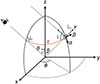Fig. 2. Geometry for scattering. Photons emerging from a differential surface area (gray region; θ and ϕ in the observer’s frame) and scattered into the observer’s direction at an angle χ are observed on the x-z surface with an angle of θobs from the z axis.

and

$$\begin{array}{cc}\hfill P& =\sqrt{q_{\mathrm{obs}}^2+u_{\mathrm{obs}}^2},\hfill \end{array}$$(17)

$$\begin{array}{cc}\hfill {\theta }_P& =\frac{1}{2}{tan}^{-1}\left(\frac{u_{\mathrm{obs}}}{q_{\mathrm{obs}}}\right).\hfill \end{array}$$(18)

2.3.1. Radiation from the photosphere in the radial direction of the CSM disk (τ_csm, r(r_sh) > 1)

We calculated the Stokes parameters of the radiation from the photosphere in the radial direction of the CSM disk by integrating the contributions from each differential surface area across the photosphere. In this subsection, we consider cases with τ_csm, r(r_sh) > 1, where there is a photosphere in the unshocked CSM. The flux and intensity of the radiation from the photosphere with the luminosity L_ph are written as follows:

$$\begin{array}{cc}\hfill f_{\mathrm{ph}}& =\frac{L_{\mathrm{ph}}}{{\displaystyle {\int }_0^{2\pi }}\mathrm{d}\varphi {\displaystyle {\int }_{\pi /2-{\theta }_{\mathrm{disk}}}^{\pi /2+{\theta }_{\mathrm{disk}}}}\mathrm{d}\theta (r_{\mathrm{ph}}^{2}sin\theta )},\hfill \\ \hfill & =\frac{L_{\mathrm{ph}}}{4\pi r_{\mathrm{ph}}^{2}sin{\theta }_{\mathrm{disk}}},\hfill \end{array}$$(19)

$$\begin{array}{cc}\hfill I_{\mathrm{ph}}& =\frac{f_{\mathrm{ph}}}{{\displaystyle {\int }_0^{2\pi }}\mathrm{d}\varphi {\displaystyle {\int }_0^{\pi /2}}\mathrm{d}\theta (sin\theta )},\hfill \\ \hfill & =\frac{L_{\mathrm{ph}}}{8{\pi }^2{r}_{\mathrm{ph}}^{2}sin{\theta }_{\mathrm{disk}}}.\hfill \end{array}$$(20)

We assume that all photons emerging from the photosphere in the radial direction of the CSM disk are unpolarized and are subsequently scattered once above the photosphere into random directions, including cases that do not change the directions of photons before and after the scattering. Photons scattered into the observer’s direction are detected. First, we considered such photons from the differential surface area at (θ, ϕ) in the Cartesian x–y–z coordinate (see Figure 2). Here, the observer is on the x-z surface with the angle of θ_obs from the z axis. The spherical α–β–γ coordinate is defined toward the direction normal to the differential surface area at (θ,ϕ) on the photosphere, as in Figure 2.

The Stokes parameters of such photons from a differential surface area at (θ, ϕ) in the spherical α–β–γ coordinate (I_total, Q_total, and U_total) can be calculated as shown in Appendix A:

$$\begin{array}{c}\hfill \{\begin{array}{c}{I}_{\mathrm{total}}(\chi )=I_{\mathrm{ph}}(\frac{9}{8}-\frac{3}{16}{sin}^2\chi ),\hfill \\ Q_{\mathrm{total}}(\chi )=-\frac{3}{16}{I}_{\mathrm{ph}}{sin}^2\chi ,\hfill \\ U_{\mathrm{total}}(\chi )=0,\hfill \end{array}\end{array}$$(21)

where χ is the angle between the unit vector n normal to the differential surface area at (θ,ϕ) on the photosphere and the unit vector for the observer’s direction, n_obs (see also Figure 2). Using the law of cosines in spherical trigonometry, this angle is expressed as

$$\begin{array}{c}\hfill cos\chi =\mathit{n}·{\mathit{n}}_{\mathrm{obs}}=sin{\theta }_{\mathrm{obs}}sin\theta cos\varphi +cos{\theta }_{\mathrm{obs}}cos\theta .\end{array}$$(22)

The Stokes parameters of these photons in the observer’s frame (I_{obs − frame}, Q_{obs − frame}, and U_{obs − frame}) are derived by rotating the Stokes parameters defined in the spherical α − β − γ coordinate (I_total, Q_total, and U_total) with angle χ as follows:

$$\begin{array}{cc}\hfill \left(\begin{array}{c}{I}_{\mathrm{obs}-\mathrm{frame}}\\ Q_{\mathrm{obs}-\mathrm{frame}}\\ U_{\mathrm{obs}-\mathrm{frame}}\end{array}\right)& =\mathbb{L}(\pi -i_2)\left(\begin{array}{c}{I}_{\mathrm{total}}\\ Q_{\mathrm{total}}\\ U_{\mathrm{total}}\end{array}\right)\hfill \\ \hfill & =\left(\begin{array}{c}{I}_{\mathrm{total}}\\ Q_{\mathrm{total}}cos2i_2-U_{\mathrm{total}}sin2i_2\\ Q_{\mathrm{total}}sin2i_2+U_{\mathrm{total}}cos2i_2\end{array}\right).\hfill \end{array}$$(23)

Here, 𝕃(ψ) is the rotation matrix:

$$\begin{array}{c}\hfill \mathbb{L}(\psi )=\left(\begin{array}{ccc}1& 0& 0\\ 0& cos2\psi & sin2\psi \\ 0& -sin2\psi & cos2\psi \end{array}\right).\end{array}$$(24)

Then, we derived the Stokes parameters of the radiation from the photosphere in the radial direction of the CSM disk (⟨I_ph⟩, ⟨Q_ph⟩, and ⟨U_ph⟩, defined in the observer’s frame, i.e., in the Cartesian x-y-z coordinate) by integrating all contributions from each differential surface area across the photosphere visible to the observer. The integration area is the photosphere above the surface perpendicular to the observer’s direction, n_obs, passing through the origin of the x-y-z coordinate system (see Figure 3). Here, the value of the polar angle (θ₀) corresponding to the direction perpendicular to the observer’s line of sight, at a given azimuthal angle (ϕ), is derived from the right-angle relationship as follows:

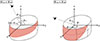Fig. 3. Schematic illustration for the integration of the Stokes parameters. The red hatches show the areas of the photosphere on the disk edge visible to the observer for cases with different combinations of θobs and θdisk.

$$\begin{array}{c}\hfill tan{\theta }_0=-\frac{1}{cos\varphi }\frac{1}{tan{\theta }_{\mathrm{obs}}}=\frac{tan({\theta }_{\mathrm{obs}}+\pi /2)}{cos\varphi }.\end{array}$$(25)

In cases with θ_obs < θ_disk, we thus derive the Stokes parameters as follows:

$$\begin{array}{c}\hfill ⟨I_{\mathrm{ph}}⟩={\displaystyle {\int }_0^{2\pi }}\mathrm{d}\varphi {\displaystyle {\int }_{\pi /2-{\theta }_{\mathrm{disk}}}^{{\theta }_0}}\mathrm{d}\theta (I_{\mathrm{obs}-\mathrm{frame}}sin\theta ),\\ \hfill ⟨Q_{\mathrm{ph}}⟩={\displaystyle {\int }_0^{2\pi }}\mathrm{d}\varphi {\displaystyle {\int }_{\pi /2-{\theta }_{\mathrm{disk}}}^{{\theta }_0}}\mathrm{d}\theta (Q_{\mathrm{obs}-\mathrm{frame}}sin\theta ),\\ \hfill ⟨U_{\mathrm{ph}}⟩={\displaystyle {\int }_0^{2\pi }}\mathrm{d}\varphi {\displaystyle {\int }_{\pi /2-{\theta }_{\mathrm{disk}}}^{{\theta }_0}}\mathrm{d}\theta (U_{\mathrm{obs}-\mathrm{frame}}sin\theta ).\end{array}$$

In the cases where θ_obs > θ_disk, we define the azimuthal angles of the crossing points between the photosphere and the bottom (θ = π/2 + θ_disk) and top (θ = π/2 − θ_disk) disk corners as ϕ₀ and ϕ₁, respectively (see Figure 3). We calculate the Stokes parameters as follows:

$$\begin{array}{cc}\hfill ⟨I_{\mathrm{ph}}⟩& ={\displaystyle {\int }_0^{{\varphi }_0}}\mathrm{d}\varphi {\displaystyle {\int }_{\pi /2-{\theta }_{\mathrm{disk}}}^{\pi /2+{\theta }_{\mathrm{disk}}}}\mathrm{d}\theta (I_{\mathrm{obs}-\mathrm{frame}}sin\theta )\hfill \\ \hfill & +{\displaystyle {\int }_{{\varphi }_0}^{{\varphi }_1}}\mathrm{d}\varphi {\displaystyle {\int }_{\pi /2-{\theta }_{\mathrm{disk}}}^{{\theta }_0}}\mathrm{d}\theta (I_{\mathrm{obs}-\mathrm{frame}}sin\theta )\hfill \\ \hfill & +{\displaystyle {\int }_{2\pi -{\varphi }_1}^{2\pi -{\varphi }_0}}\mathrm{d}\varphi {\displaystyle {\int }_{\pi /2-{\theta }_{\mathrm{disk}}}^{{\theta }_0}}\mathrm{d}\theta (I_{\mathrm{obs}-\mathrm{frame}}sin\theta )\hfill \\ \hfill & +{\displaystyle {\int }_{2\pi -{\varphi }_0}^{2\pi }}\mathrm{d}\varphi {\displaystyle {\int }_{\pi /2-{\theta }_{\mathrm{disk}}}^{\pi /2+{\theta }_{\mathrm{disk}}}}\mathrm{d}\theta (I_{\mathrm{obs}-\mathrm{frame}}sin\theta ),\hfill \\ \hfill & =2{\displaystyle {\int }_0^{{\varphi }_0}}\mathrm{d}\varphi {\displaystyle {\int }_{\pi /2-{\theta }_{\mathrm{disk}}}^{\pi /2+{\theta }_{\mathrm{disk}}}}\mathrm{d}\theta (I_{\mathrm{obs}-\mathrm{frame}}sin\theta )\hfill \end{array}$$(26)

$$\begin{array}{cc}& +2{\displaystyle {\int }_{{\varphi }_0}^{{\varphi }_1}}\mathrm{d}\varphi {\displaystyle {\int }_{\pi /2-{\theta }_{\mathrm{disk}}}^{{\theta }_0}}\mathrm{d}\theta (I_{\mathrm{obs}-\mathrm{frame}}sin\theta ),\hfill \\ \hfill ⟨Q_{\mathrm{ph}}⟩& =2{\displaystyle {\int }_0^{{\varphi }_0}}\mathrm{d}\varphi {\displaystyle {\int }_{\pi /2-{\theta }_{\mathrm{disk}}}^{\pi /2+{\theta }_{\mathrm{disk}}}}\mathrm{d}\theta (Q_{\mathrm{obs}-\mathrm{frame}}sin\theta )\hfill \end{array}$$(27)

$$\begin{array}{cc}& +2{\displaystyle {\int }_{{\varphi }_0}^{{\varphi }_1}}\mathrm{d}\varphi {\displaystyle {\int }_{\pi /2-{\theta }_{\mathrm{disk}}}^{{\theta }_0}}\mathrm{d}\theta (Q_{\mathrm{obs}-\mathrm{frame}}sin\theta ),\hfill \\ \hfill ⟨U_{\mathrm{ph}}⟩& =2{\displaystyle {\int }_0^{{\varphi }_0}}\mathrm{d}\varphi {\displaystyle {\int }_{\pi /2-{\theta }_{\mathrm{disk}}}^{\pi /2+{\theta }_{\mathrm{disk}}}}\mathrm{d}\theta (U_{\mathrm{obs}-\mathrm{frame}}sin\theta )\hfill \\ \hfill & +2{\displaystyle {\int }_{{\varphi }_0}^{{\varphi }_1}}\mathrm{d}\varphi {\displaystyle {\int }_{\pi /2-{\theta }_{\mathrm{disk}}}^{{\theta }_0}}\mathrm{d}\theta (U_{\mathrm{obs}-\mathrm{frame}}sin\theta ).\hfill \\ \hfill \end{array}$$(28)

In both cases, we get the following formulas:

$$\begin{array}{cc}\hfill ⟨I_{\mathrm{ph}}⟩& =\frac{\pi I_{\mathrm{ph}}}{16}[3(11-{cos}^2{\theta }_{\mathrm{obs}})sin{\theta }_{\mathrm{disk}}\hfill \\ \hfill & -(1-3{cos}^2{\theta }_{\mathrm{obs}}){sin}^3{\theta }_{\mathrm{disk}}],\hfill \end{array}$$(30)

$$\begin{array}{cc}\hfill ⟨Q_{\mathrm{ph}}⟩& =\frac{3\pi I_{\mathrm{ph}}}{16}{sin}^2{\theta }_{\mathrm{obs}}{cos}^2{\theta }_{\mathrm{disk}}sin{\theta }_{\mathrm{disk}},\hfill \end{array}$$(31)

$$\begin{array}{cc}\hfill ⟨U_{\mathrm{ph}}⟩& =0.\hfill \end{array}$$(32)

2.3.2. Radiation from the photosphere in the radial direction of the CSM disk (τ_csm, r(r_sh) < 1)

In cases with τ_csm, r(r_sh) < 1, where there is a photosphere in the shocked region, we assume that unpolarized photons emerge from the shocked region with L_ph = L_sh. A part of these photons are then scattered with a probability proportional to τ_csm, r(r_sh). Thus, we calculate ⟨Q_ph⟩ and ⟨U_ph⟩ using the same formulas as in the previous subsection, but multiply them by τ_csm, r(r_sh).

2.3.3. Radiation from the photosphere at the surface of the CSM disk

The polarization degree of the radiation from the photosphere at the surface of the CSM disk depends on the exact density distribution of the surface of the disk. In this paper, we assume that the boundary of the CSM disk is sharply defined by a sudden density drop from ρ_disk to zero, and that the radiation from the disk surface is unpolarized, for simplicity. Thus, we get the following formulas:

$$\begin{array}{cc}\hfill ⟨I_{\mathrm{surface}}⟩& =\frac{L_{\mathrm{surface}}}{4\pi (1-sin{\theta }_{\mathrm{disk}})},\hfill \end{array}$$(33)

$$\begin{array}{cc}\hfill ⟨Q_{\mathrm{surface}}⟩& =0,\hfill \end{array}$$(34)

$$\begin{array}{cc}\hfill ⟨U_{\mathrm{surface}}⟩& =0.\hfill \end{array}$$(35)

We note that, in reality, the density distribution at the disk boundary should not be sharply defined and thus the radiation from the disk surface can be polarized to some extent.

3. Results

3.1. Polarization properties

The obtained polarization angle, defined as measured from the z-axis, remains constant at zero over time. This means that the polarization angle consistently aligns with the polar axis of the CSM disk on the plane of the sky in our configuration (see Figures 1 and 2). Since we assumed that the radiation from the surface of the CSM disk is unpolarized (see Equations 33-35), it can only reduce the net polarization degree by adding unpolarized radiation and cannot affect the polarization angle. The only source of polarization is the radiation from the photosphere, where ⟨Q_ph⟩ is positive and ⟨U_ph⟩ is zero (see Equations (30)–(32)). As a result, the polarization angle (Equation 18) remains fixed at zero degrees (θ_P = 0). This outcome is consistent with expectations, as the spatial relationship between the observer and the scattering bodies remains constant over time.

Figure 4 shows the time evolution of the polarization degree for cases with fiducial parameters of θ_disk = 60 degrees, s = 2.0, M_csm = 2 × 10⁻³ M_⊙, and r_out = 3 × 10¹⁴ cm, but with different values of θ_obs. Higher values of θ_obs (i.e., viewing angles closer to the equatorial plane) produce greater degrees of polarization. As the viewing angle decreases (i.e., viewing angles closer to the pole of the CSM disk), the spatial distribution of scattered photons becomes more circularly symmetric. This results in a reduced net polarization due to the cancellation of the linear polarization components. The decline and eventual disappearance of the polarization signals correspond to the times when the optical depth in front of the interaction shock drops below unity (τ_csm, r(r_sh) = 1), and when the interaction shock reaches the outer edge of the confined CSM, respectively. Thus, these times do not depend on the viewing angle. In cases where the observer sees the surface of the CSM disk (θ_obs ≤ π/2 − θ_disk), the net polarization is suppressed by the unpolarized radiation from the surface of the CSM disk, until the CSM becomes optically thin. Thus, we see gradual increase in polarization until ∼3 days after the explosion in the cases with θ_obs ≤ 30 in Figure 4. The observed polarization of SN 2023ixf favors θ_obs = 40 degrees for the assumed values of the other parameters.

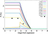Fig. 4. Time evolution of the polarization degree. The cases with parameters of θdisk = 60 degrees, s = 2.0, Mcsm = 2 × 10−3 M⊙, and rout = 3 × 1014 cm but various values of θobs are shown. The black points show the observed polarization in SN 2023ixf (Vasylyev et al. 2023, see Section 3.2).

Figure 5 shows the time evolution of the polarization degree for the cases with the fiducial parameters of θ_obs = 40 degrees, s = 2.0, M_csm = 2 × 10⁻³ M_⊙, and r_out = 3 × 10¹⁴ cm, but with different values of θ_disk. For smaller opening angle of the CSM disk, the peak polarization degree is larger. This is because the average scattering angles become closer to 90 degrees, whose scattering creates the largest polarization degree, for smaller values of θ_disk. There are also polarization rises, as in Figure 4, for the cases with θ_obs ≤ π/2 − θ_disk (i.e., θ_disk ≤ 50). For cases with smaller θ_disk, this polarization rise is more substantial. This is because the unpolarized radiation escaping from the surface of the CSM disk is larger compared to the polarized radiation originating from the photosphere (i.e., L_surface/L_ph is larger) for cases with smaller θ_disk. The timing of the disappearance of the polarization is slightly earlier in cases with larger θ_disk. This is because the density of the CSM is smaller and thus the shock evolves faster, in cases with larger θ_disk. The observed polarizaion of SN 2023ixf would prefer θ_disk = 60 degrees for the assumed values of the other parameters.

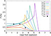Fig. 5. Time evolution of the polarization degree. The cases with parameters of θobs = 40 degrees, s = 2.0, Mcsm = 2 × 10−3 M⊙, and rout = 3 × 1014 cm but various values of θdisk are shown. The black points are the same as in Figure 4.

Figure 6 shows the time evolution of the polarization degree for the cases with fiducial parameters of θ_obs = 40 degrees, θ_disk = 60 degrees, s = 2.0, and r_out = 3 × 10¹⁴ cm, but with different values of M_csm. Since we observe the system through the unshocked CSM for these assumed parameters, the maximum polarization degree determined by the geometry between the observer and the scattering bodies does not change for all the cases here. On the other hand, the timing of the disappearance of the polarization largely depends on the value of the CSM mass. This is because the shock evolution is slower in cases with higher values of M_csm. Since the location of the interaction shock when the unshocked CSM becomes optically thin is closer to the outer edge of the CSM disk, the decline in polarization is faster for cases with higher M_csm. The observed polarization of SN 2023ixf favors M_csm = 10⁻³ M_⊙ for the assumed values of the other parameters.

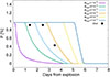Fig. 6. Time evolution of the polarization degree. The cases with parameters of θobs = 40 degrees, θdisk = 60 degrees, s = 2.0, and rout = 3 × 1014 cm but various values of Mcsm are shown. The black points are the same as in Figure 4.

Figure 7 shows the time evolution of the polarization degree for the cases with the fiducial parameters of θ_obs = 40 degrees, θ_disk = 60 degrees, M_csm = 2 × 10⁻³ M_⊙, and s = 2.0, but with different values of r_out. Since the shock evolution is identical for all the cases here, the different values of r_out result in different times of the disappearance of the polarization. On the other hand, the location where the unshocked CSM becomes optically thin does not strongly depend on the outer radius of the CSM disk (∼2 × 10¹⁴ cm for the assumed density distribution), creating similar times of the polarization decline. The observed polarization of SN 2023ixf favors r_out = 2 × 10¹⁴ cm for the assumed values of the other parameters.

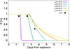Fig. 7. Time evolution of the polarization degree. The cases with parameters of θobs = 40 degrees, θdisk = 60 degrees, Mcsm = 2 × 10−3 M⊙, and s = 2.0 but various values of rout are shown. The black points are the same as in Figure 4.

Figure 8 shows the time evolution of the polarization degree for the cases with the fiducial parameters of θ_obs = 40 degrees, θ_disk = 60 degrees, M_csm = 2 × 10⁻³ M_⊙, and r_out = 3 × 10¹⁴ cm, but with different values of s. These models do not produce much difference. Since we assume the single-scattering approximation, the distribution of the scattering bodies does not affect the polarization degree. Although the difference of s can affect the evolution of the interaction shock, the difference in the results is not significant for the assumed values of the parameters.

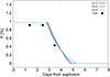Fig. 8. Time evolution of the polarization degree. The cases with parameters of θobs = 40 degrees, θdisk = 60 degrees, Mcsm = 2 × 10−3 M⊙, and rout = 3 × 1014 cm but various values of s are shown. The black points are the same as in Figure 4.

3.2. Characteristic values of the polarization and CSM parameter estimation

As shown in the previous subsection, the temporal evolution of polarization in Type II SNe with confined CSM can be used to roughly estimate the CSM parameters. We consider the following characteristic quantities: polarization maximum (P_max, the maximum polarization degree); rise time (t_rise, the time from the explosion until polarization maximum); duration (t_duration, the time from the explosion until polarization decline begins), decline time (t_decline, the time from polarization decline onset to its disappearance). Here, in cases without a polarization rise (i.e., a constant polarization at early phases), we set t_rise to zero.

The maximum polarization degrees are primarily determined by the values θ_obs and θ_disk, rather than M_csm, r_out, and s. Since maximum polarization is determined by the average scattering angles of the photons emerging from the photosphere, the geometry between the photosphere and the observer (related to θ_obs) and the shape of the photosphere (related to θ_disk) are the important factors. Figure 9a shows the maximum polarization degrees for models with varying values of θ_obs and θ_disk, assuming M_csm = 2 × 10⁻³ M_⊙, r_out = 3 × 10¹⁴ [cm], and s = 2. Smaller opening angles and larger viewing angles result in higher maximum polarization degrees. At the same time, the polarization rise also provides a constraint for the values θ_obs and θ_disk. When there is a rise, we obtain the constraint θ_obs ≤ π/2 − θ_disk. Otherwise, the viewing angle is larger than π/2 − θ_disk. Figure 9b shows the rise time of the polarization, which strongly correlates with θ_disk and thus can be used for estimating its value.

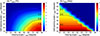Fig. 9. Parameter dependence of the maximum polarization degree (Pmax) and the rise time (trise). (a) Pmax for cases with Mcsm = 2 × 10−3 M⊙, rout = 3 × 1014 cm, and s = 2 but various values of θobs and θdisk. (b) Same as panel (a), but for trise. The region with θobs ≥ π/2 − θdisk (i.e., cases with edge-on views) corresponds to trise = 0. The wavy pattern around θobs = π/2 − θdisk is an artifact caused by the limited size of the computational grid.

The duration and decline time of the polarization are more sensitive to the values of M_csm and r_out than to those of θ_obs, θ_disk, or s. Figure 10a shows the duration and decline time for models with varying values of M_csm and r_out, assuming θ_obs = 40 degrees, θ_disk = 60 degrees, and s = 2. The duration more strongly correlates with M_csm than with r_out, whereas the decline time shows the opposite trend. Therefore, by measuring the duration and decline time with polarimetric observations, we can constrain the values of M_csm and r_out.

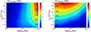Fig. 10. Parameter dependence of the duration (tduration) and decline time (tdecline) of the polarization. (a) tduration for cases with θobs = 40 degrees, θdisk = 60 degrees, and s = 2 but various values of Mcsm and rout. (b) Same as panel (a), but for tdecline.

Here, we consider applying these results to observations of Type II SN 2023ixf – the only SN that has early-time polarimetric observations with good temporal coverage – to derive its CSM parameters. SN 2023ixf shows polarization with time-varying degrees and angles (Vasylyev et al. 2023, 2025). Following Vasylyev et al. (2023, 2025), we interpret the first component of the observed polarization – with polarization angles of ∼160 degrees observed until ∼4 days – as originating from the confined CSM modeled in this study. For SN 2023ixf, we roughly estimate the values of the characteristic parameters as follows: P_max ∼ 0.9 %, t_rise ≲ 1 day, t_duration ∼ 2.5 ± 0.5 days, t_decline ∼ 2 ± 0.5 days.

Based on P_max and t_rise values, we estimate the good-fit values of θ_obs and θ_disk as ≳40 degrees and ∼60 degrees, respectively, using the relations in Figure 9 (see Figure 11a). We note that, as discussed in the next section, the polarization degrees obtained from our calculations may be overestimated due to the single-scattering assumption (see Section 4 for details). Therefore, the actual value of θ_disk might be slightly lower. If we take the region with 1 ≤ P_max ≤ 3 % and t_rise ≤ 1 day, the good-fit values would be θ_obs ≲ 40 degrees and 50 ≲ θ_disk ≲ 60 degrees (see the blue hatched region in Figure 11a). Based on the values of t_duration and t_decline, we estimate good-fit values of M_csm and r_out as ∼2 × 10⁻³ M_⊙ and ∼3 × 10¹⁴ cm, respectively, using the relations in Figure 10 (see Figure 11b).

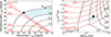Fig. 11. Application of the observed polarization of Type II SN 2023ixf to the models in Figures 9 and 10. The black dots show our adopted good-match values, while the blue regions correspond to the regions with the best-fit values.

The observed polarization angle of ∼160 degrees suggests that the polar axis of the confined CSM disk of SN 2023ixf – if it has a disk-like distribution – is tilted by ∼160 degrees from the north-south direction on the night sky. Interestingly, this orientation correlates with the axis of the asymmetric structure of the SN 2023ixf explosion (Vasylyev et al. 2025). This alignment may indicate that the mechanisms creating the aspherical structures of both the confined CSM and the SN ejecta are related. Thus, the formation of the confined CSM might be driven by processes intrinsic to the progenitor star itself, rather than by interactions with a companion star, unless all the axes of the explosion, the CSM disk, and the companion orbit are aligned. This should be investigated with more observations of early polarimetry of Type II SNe.

4. Limitations of the calculations

In this section, we discuss the limitations of our methodology to predict the polarization signals from confined CSM in Type II SNe. Our calculation method has several simplifications. The biggest is the assumption of single scattering (see Section 2). In our calculations, we assumed that the location of the photosphere corresponds to τ_csm, r(r_ph) = 1, and that the photons emerging from the photosphere are scattered only once, as the atmosphere above it is optically thin. However, multiple scatterings can in principle occur, which reduce the polarization degree. This would depend on the configuration of scattering bodies, i.e., the locations where the last scatterings typically occur.

To roughly estimate the probability of multiple scatterings, we checked the average locations of the photon scattering events originating from the photosphere (r_scat) and assessed the optical depth from those locations to the observer (τ_scat), in the single-scattering case (see Figure 12). If this optical depth is larger than unity, the scattered photons can have additional scattering events, and thus the calculated polarization degrees can be lower than those in Section 3. When τ_csm, r(r_sh)≥1, the average radius of the scatterings is estimated by τ_csm, r(r_scat) = 1/2. Thus, we get

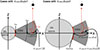Fig. 12. Schematic illustration of our calculations for τscat.

$$\begin{array}{c}\hfill r_{\mathrm{scat}}={(r_{\mathrm{out}}^{-(s-1)}+\frac{s-1}{2{\kappa }_{\mathrm{es}}D})}^{-1/(s-1)},\end{array}$$(36)

and

$$\begin{array}{c}\hfill {\tau }_{\mathrm{csm},\mathrm{h}}(r_{\mathrm{scat}})={\theta }_{\mathrm{disk}}({\kappa }_{\mathrm{es}}D{r}_{\mathrm{out}}^{-(s-1)}+\frac{s-1}{2}).\end{array}$$(37)

For simplicity, we assume the optical depth from the average locations of the scattering events to the observer with θ_obs, as follows:

$$\begin{array}{c}\hfill {\tau }_{\mathrm{scat}}({\theta }_{\mathrm{obs}})=(1-cos{\theta }_{\mathrm{obs}}){\tau }_{\mathrm{csm},\mathrm{r}}(r_{\mathrm{scat}})+cos{\theta }_{\mathrm{obs}}{\tau }_{\mathrm{csm},\mathrm{h}}(r_{\mathrm{scat}}).\end{array}$$(38)

When τ_csm, r(r_sh) < 1, we define r_scat using τ_csm, r(r_scat) = 1/2 × τ_csm, r(r_sh), as follows:

$$\begin{array}{c}\hfill r_{\mathrm{scat}}={(\frac{1}{2}{r}_{\mathrm{sh}}^{-(s-1)}+\frac{1}{2}{r}_{\mathrm{out}}^{-(s-1)})}^{-1/(s-1)}.\end{array}$$(39)

Thus,

$$\begin{array}{c}\hfill {\tau }_{\mathrm{csm},\mathrm{h}}(r_{\mathrm{scat}})=\frac{{\kappa }_{\mathrm{es}}D{\theta }_{\mathrm{disk}}}{2}(r_{\mathrm{sh}}^{-(s-1)}+r_{\mathrm{out}}^{-(s-1)}),\end{array}$$(40)

and

$$\begin{array}{cc}\hfill {\tau }_{\mathrm{scat}}({\theta }_{\mathrm{obs}})& ={\kappa }_{\mathrm{es}}D(\frac{1-cos{\theta }_{\mathrm{obs}}}{2(s-1)}+\frac{{\theta }_{\mathrm{disk}}cos{\theta }_{\mathrm{obs}}}{2})r_{\mathrm{sh}}^{-(s-1)}\hfill \\ \hfill & +{\kappa }_{\mathrm{es}}D(-\frac{1-cos{\theta }_{\mathrm{obs}}}{2(s-1)}+\frac{{\theta }_{\mathrm{disk}}cos{\theta }_{\mathrm{obs}}}{2})r_{\mathrm{out}}^{-(s-1)}.\hfill \end{array}$$(41)

Figure 13 shows the time evolution of τ_scat for different values of θ_obs and θ_disk. When there is a photosphere (i.e., τ_csm, r(r_sh)≥1), the locations of the scattering events are constant with time; thus, the values of τ_scat are also constant. Once the shocked shell reaches the location where τ_csm, r = 1, the optical depth at the scattering locations gradually decreases over time, until the shock reaches the outer edge of the confined CSM. When τ_scat is roughly greater than unity, the calculated polarization degrees in the single-scattering configuration is overestimated. The maximum values of τ_scat for different values of θ_obs and θ_disk are shown in Figure 14. Cases with smaller viewing angles and larger half-opening angles of the CSM disk have significantly higher values of τ_scat than unity. Thus, the calculated polarization degrees for such cases should in reality be reduced by multiple scatterings. On the other hand, cases with higher calculated polarization degrees (i.e., with larger viewing angles and smaller half-opening angles) are less affected by multiple scatterings (see also Figure 9).

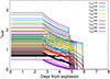Fig. 13. Time evolution of τscat in cases with different values of θobs and θdisk, with Mcsm = 10−3 M⊙, rout = 2 × 1014 [cm], and s = 2.

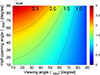Fig. 14. Maximum τscat for cases with different values of θobs and θdisk, with Mcsm = 10−3 M⊙, rout = 2 × 1014 [cm], and s = 2.

The good-fit case for SN 2023ixf (with θ_obs = 40 degrees, θ_disk = 60 degrees, M_csm = 10⁻³ M_⊙, r_out = 2 × 10¹⁴ cm, and s = 2.0) has τ_scat ∼ 2. Therefore, taking multiple-scattering effects into account, the realistic parameters for the confined CSM in SN 2023ixf would require a slightly larger viewing angle and/or a slightly smaller half-opening angle. We note that this is a very rough estimate of possible multiple-scattering effects, ignoring realistic distribution of the CSM. Thus, we need to conduct multidimensional radiative transfer calculations to obtain accurate polarization values.

Another simplification that might affect our results is the polarization degree of radiation originating from the CSM disk surface, which we assume to be zero. In reality, this radiation can exhibit a nonnegligible amount of polarization and could affect polarization degrees at early phases (i.e., when τcsm, r(r_sh) > 1) for cases with θ_obs ≤ π/2 − θ_disk. We note that this modification does not change the maximum polarization degrees, the timing of polarization rises, or the duration of polarization. In addition, since we assume that the main radiation source is the interaction between the SN ejecta and the CSM – ignoring the contribution from the SN ejecta – results for cases with a smaller amount of CSM may be less reliable.

5. Conclusion

We modeled the polarization signals produced by electron scattering in a Type II SN with a confined, disk-like CSM. In this system, the calculated polarization angle remains constant at zero degrees, which is parallel to the axis of the CSM disk, regardless of the parameters of the confined CSM. The temporal evolution of the polarization degree varies depending on the parameters of the confined CSM on a timescale of ≲10 days. The general behavior is as follows. Initially, the polarization degree remains constant or gradually increases to a few percent while the unshocked CSM in front of the interaction shock remains optically thick. It then reaches a peak as the unshocked CSM becomes optically thin. Finally, polarization declines and eventually vanishes as the interaction shock reaches the outer edge of the CSM disk. The results demonstrate that early-time polarization in Type II SNe can effectively probe the geometry and properties of confined CSM. In particular, the maximum degree and polarization rise time can constrain the viewing and opening angle of the CSM disk, while the duration and decline time can constrain the mass and extension of the CSM disk.

As a concrete application to observations, we apply the models to the observed polarization of Type II SN 2023ixf and find that it can be explained by a disk-like CSM with the following parameters: viewing angle θ_obs ≳ 40 degrees, disk half-opening angle θ_disk ∼ 50 − 60 degrees, CSM mass M_csm ∼ 2 × 10⁻³ M_⊙, and outer CSM disk radius r_out ∼ 3 × 10¹⁴ cm. In addition, the alignment between the explosion asymmetry and the CSM disk of SN 2023ixf may suggest a common origin for these asymmetric structures, possibly tied to the progenitor star rather than companion interaction. Early polarimetry of Type II SNe will be essential to test this scenario. Furthermore, the developed method is broadly applicable to various objects with scattering-dominated photospheres, offering a powerful tool for investigating their geometries.

Acknowledgments

We thank Masaomi Tanaka and Avinash Singh for valuable discussions and insights. The authors wish to acknowledge CSC – IT Center for Science, Finland, for computational resources. This research is supported by the Finnish Ministry of Education and Culture and CSC – IT Centre for Science (Decision diary number OKM/10/524/2022). T.N. acknowledges support from the Research Council of Finland projects 324504, 328898 and 353019.K.M. acknowledges support from JSPS KAKENHI grant (JP24KK0070, JP24H01810).

References

Appendix A: Polarization from a unit area on a photosphere

We consider a unit area on a “photosphere" in scattering-dominated gas. In this paper, we define the photosphere as the region where the optical depth, measured from the observer, equals unity. We assume that all photons at the photosphere are unpolarized and are scattered once above the photosphere. We note that possible additional scatterings after the first (i.e., multiple scatterings) are ignored. The Cartesian α-β-γ coordinate is defined on a unit area of the photosphere as in Figure A.1. We use the spherical θ-ϕ coordinate defined in the Cartesian α-β-γ coordinate (see Figure A.1). The observer is on the α-γ surface with the viewing angle, χ, from the γ axis (i.e., (θ,ϕ) = (χ,0)). The emerging flux at the unit area of the photosphre is expressed as f_in, and its intensity to the perpendicular direction towards the area (i.e., the γ direction) as I_in. Since the intensity toward the angle θ from the γ direction (I₀) is I_in cos θ, we get the relation between f_in and I_in as follows:

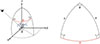Fig. A.1. Geometry for scattering. The spherical θ-ϕ coordinate is defined in the Cartesian α-β-γ coordinate. A photon emerging from a unit area (gray region) at the origin to a direction of (θ, ϕ) is scattered toward observer (χ,0).

$$\begin{array}{cc}\hfill f_{\mathrm{in}}& ={\displaystyle {\int }_0^{\pi /2}}{I}_0\mathrm{d}\theta {\displaystyle {\int }_0^{2\pi }}\mathrm{d}\varphi =2\pi I_{\mathrm{in}},\hfill \end{array}$$(A.1)

$$\begin{array}{cc}\hfill \therefore I_{\mathrm{in}}& =\frac{f_{\mathrm{in}}}{2\pi }.\hfill \end{array}$$(A.2)

We consider the photons that are emitted for a unit time to the direction of (θ,ϕ) from this unit area, whose Stokes parameters are (𝕊₀ = (I₀, 0, 0)). Some of these photons would be scattered to the observer’s direction, (θ, ϕ) = (χ, 0), at a certain radius, whose Stokes parameters are denoted as (𝕊₁ = (I₁, Q₁, U₁)). We can calculate this conversion of these Stokes vectors of the photons before and after the scatterings, using the scattering matrix (ℝ(Θ)) and the rotation matrix (𝕃(ψ)), as follows:

$$\begin{array}{c}\hfill {\mathbb{S}}_1=\mathbb{L}(\pi -i_2)\mathbb{R}(\mathrm{\Theta })\mathbb{L}(-i_1){\mathbb{S}}_0,\end{array}$$(A.3)

where,

$$\begin{array}{c}\hfill \mathbb{R}(\mathrm{\Theta })=\alpha \left(\begin{array}{ccc}{cos}^2(\mathrm{\Theta })+1& {cos}^2(\mathrm{\Theta })-1& 0\\ {cos}^2(\mathrm{\Theta })-1& {cos}^2(\mathrm{\Theta })+1& 0\\ 0& 0& 2cos\mathrm{\Theta }\end{array}\right),\mathbb{L}(\psi )=\left(\begin{array}{ccc}1& 0& 0\\ 0& cos2\psi & sin2\psi \\ 0& -sin2\psi & cos2\psi \end{array}\right),\end{array}$$(A.4)

and the Θ is the angle between the angles before and after the scatterings, and the angles of i₁ and i₂ are defined as in Figure A.1. Based on the spherical trigonometry, we can derive these angles:

$$\begin{array}{cc}\hfill cos\mathrm{\Theta }& =cos\chi cos\theta +sin\chi sin\theta cos\varphi ,\hfill \end{array}$$(A.5)

$$\begin{array}{cc}\hfill cos{i}_2& =\frac{cos\theta -cos\chi cos\mathrm{\Theta }}{sin\chi sin\mathrm{\Theta }}.\hfill \end{array}$$(A.6)

Using these values, we obtain the conversion equations.

$$\begin{array}{c}\hfill \{\begin{array}{c}{I}_1(\theta ,\varphi )=\alpha I_0(1+{cos}^2\chi {cos}^2\theta +2cos\chi sin\chi cos\theta sin\theta cos\varphi +{sin}^2\chi {sin}^2\theta {cos}^2\varphi ),\hfill \\ Q_1(\theta ,\varphi )=\alpha I_0(-1+2{sin}^2\theta +{cos}^2\chi {cos}^2\theta +2cos\chi sin\chi cos\theta sin\theta cos\varphi +({sin}^2\chi -2){sin}^2\theta {cos}^2\varphi ),\hfill \\ U_1(\theta ,\varphi )=-2\alpha I_0(sin\chi cos\theta sin\theta sin\varphi -cos\chi {sin}^2\theta cos\varphi sin\varphi ).\hfill \end{array}\end{array}$$(A.7)

Next, we consider all the contribution from all the photons that are emitted to all directions from the unit area during a unit time. We can simply integrate all the contribution to the total Stokes parameters from all the photons that are scattered to the observer’s direction, as follows:

$$\begin{array}{cc}\hfill I_{\mathrm{total}}(\chi )& ={\displaystyle {\int }_0^{2\pi }}d\varphi {\displaystyle {\int }_0^{\pi /2}}d\theta \{I_1(\theta ,\varphi )sin\theta \},\hfill \end{array}$$(A.8)

$$\begin{array}{cc}& =\alpha I_{\mathrm{in}}{\displaystyle {\int }_0^{\pi /2}}d\theta \{(sin\theta +{cos}^2\chi {cos}^2\theta sin\theta )cos\theta \left({\displaystyle {\int }_0^{2\pi }}d\varphi \right)+2cos\chi sin\chi {cos}^2\theta {sin}^2\theta ({\displaystyle {\int }_0^{2\pi }}cos\varphi d\varphi )\hfill \\ \hfill & +{sin}^2\chi cos\theta {sin}^3\theta \left({\displaystyle {\int }_0^{2\pi }}{cos}^2\varphi d\varphi \right)\},\hfill \end{array}$$(A.9)

$$\begin{array}{cc}& =\alpha \pi I_{\mathrm{in}}\{2({\displaystyle {\int }_0^{\pi /2}}cos\theta sin\theta d\theta )+2{cos}^2\chi ({\displaystyle {\int }_0^{\pi /2}}{cos}^3\theta sin\theta d\theta )+{sin}^2\chi ({\displaystyle {\int }_0^{\pi /2}}cos\theta {sin}^3\theta d\theta )\},\hfill \end{array}$$(A.10)

$$\begin{array}{cc}& =\alpha \pi I_{\mathrm{in}}(1+\frac{1}{2}{cos}^2\chi +\frac{1}{4}{sin}^2\chi ),\hfill \end{array}$$(A.11)

$$\begin{array}{cc}& =\alpha \pi I_{\mathrm{in}}(\frac{3}{2}-\frac{1}{4}{sin}^2\chi ).\hfill \end{array}$$(A.12)

$$\begin{array}{cc}\hfill Q_{\mathrm{total}}(\chi )& ={\displaystyle {\int }_0^{2\pi }}d\varphi {\displaystyle {\int }_0^{\pi /2}}d\theta \{Q_1(\theta ,\varphi )sin\theta \},\hfill \end{array}$$(A.13)

$$\begin{array}{cc}& =\alpha I_{\mathrm{in}}{\displaystyle {\int }_0^{\pi /2}}d\theta \{(-cos\theta sin\theta +2cos\theta {sin}^3\theta +{cos}^2\chi {cos}^3\theta sin\theta )\left({\displaystyle {\int }_0^{2\pi }}d\varphi \right)\hfill \\ \hfill & +2cos\chi sin\chi {cos}^2\theta {sin}^2\theta ({\displaystyle {\int }_0^{2\pi }}cos\varphi d\varphi )+({sin}^2\chi -2)cos\theta {sin}^3\theta \left({\displaystyle {\int }_0^{2\pi }}{cos}^2\varphi d\varphi \right)\},\hfill \end{array}$$(A.14)

$$\begin{array}{cc}& =\alpha \pi I_{\mathrm{in}}\{-2({\displaystyle {\int }_0^{\pi /2}}cos\theta sin\theta d\theta )+({sin}^2\chi +2)({\displaystyle {\int }_0^{\pi /2}}cos\theta {sin}^3\theta d\theta )+2{cos}^2\chi ({\displaystyle {\int }_0^{\pi /2}}{cos}^3\theta sin\theta d\theta )\},\hfill \end{array}$$(A.15)

$$\begin{array}{cc}& =\alpha \pi I_{\mathrm{in}}(-\frac{1}{2}+\frac{1}{4}{sin}^2\chi +\frac{1}{2}{cos}^2\chi ),\hfill \end{array}$$(A.16)

$$\begin{array}{cc}& =-\frac{\alpha \pi I_{\mathrm{in}}}{4}{sin}^2\chi .\hfill \end{array}$$(A.17)

$$\begin{array}{cc}\hfill U_{\mathrm{total}}(\chi )& ={\displaystyle {\int }_0^{2\pi }}d\varphi {\displaystyle {\int }_0^{\pi /2}}d\theta \{U_1(\theta ,\varphi )sin\theta \},\hfill \end{array}$$(A.18)

$$\begin{array}{cc}& =-2\alpha I_{\mathrm{in}}{\displaystyle {\int }_0^{\pi /2}}d\theta \{sin\chi {cos}^2\theta sin\theta ({\displaystyle {\int }_0^{2\pi }}sin\varphi d\varphi )-cos\chi cos\theta {sin}^3\theta ({\displaystyle {\int }_0^{2\pi }}cos\varphi sin\varphi d\varphi )\},\hfill \end{array}$$(A.19)

$$\begin{array}{cc}& =0.\hfill \end{array}$$(A.20)

Since we assume that all the photons emitted from the unit area are scattered once including the photons that are scattered to the same direction as that before the scattering, the total number of the scattered photons should be the same with that of the emitted photons from the photosphere per unit time (f_in):

$$\begin{array}{cc}\hfill f_{\mathrm{in}}& ={\displaystyle {\int }_0^{2\pi }}d\varphi {\displaystyle {\int }_0^{\pi /2}}d\chi \{I_{\mathrm{total}}(\chi )sin\chi \},\hfill \end{array}$$(A.21)

$$\begin{array}{cc}& =(2\pi I_{\mathrm{in}})\alpha \pi {\displaystyle {\int }_0^{\pi /2}}d\chi \{\frac{3}{2}sin\chi -\frac{1}{4}{sin}^3\chi \},\hfill \end{array}$$(A.22)

$$\begin{array}{ccc}& \therefore \hfill & \hfill \alpha =\frac{3}{4\pi }.\end{array}$$(A.23)

Therefore, we can calculate the Stokes parameters of the radiation from a unit area on the photosphere using the following simple formula:

$$\begin{array}{c}\hfill \{\begin{array}{c}{I}_{\mathrm{total}}(\chi )=I_{\mathrm{in}}(\frac{9}{8}-\frac{3}{16}{sin}^2\chi ),\hfill \\ Q_{\mathrm{total}}(\chi )=-\frac{3}{16}{I}_{\mathrm{in}}{sin}^2\chi ,\hfill \\ U_{\mathrm{total}}(\chi )=0.\hfill \end{array}\end{array}$$(A.24)

All Figures

Fig. 1. Schematic representation of our calculations. The radiation is generated by the interaction between the SN ejecta the disk-like CSM, with a luminosity of Lsh. A portion of this radiation escapes from the surface of the CSM disk before reaching the photosphere (indicated by the dotted lines in the CSM), with a luminosity of Lsurface, while the remaining radiation escapes from the photosphere, with a luminosity of Lph. The radiation emitted from the photosphere can be polarized due to the last scattering above the photosphere.

In the text

	Fig. 2. Geometry for scattering. Photons emerging from a differential surface area (gray region; θ and ϕ in the observer’s frame) and scattered into the observer’s direction at an angle χ are observed on the x-z surface with an angle of θobs from the z axis.
In the text

	Fig. 3. Schematic illustration for the integration of the Stokes parameters. The red hatches show the areas of the photosphere on the disk edge visible to the observer for cases with different combinations of θobs and θdisk.
In the text

	Fig. 4. Time evolution of the polarization degree. The cases with parameters of θdisk = 60 degrees, s = 2.0, Mcsm = 2 × 10−3 M⊙, and rout = 3 × 1014 cm but various values of θobs are shown. The black points show the observed polarization in SN 2023ixf (Vasylyev et al. 2023, see Section 3.2).
In the text

	Fig. 5. Time evolution of the polarization degree. The cases with parameters of θobs = 40 degrees, s = 2.0, Mcsm = 2 × 10−3 M⊙, and rout = 3 × 1014 cm but various values of θdisk are shown. The black points are the same as in Figure 4.
In the text

	Fig. 6. Time evolution of the polarization degree. The cases with parameters of θobs = 40 degrees, θdisk = 60 degrees, s = 2.0, and rout = 3 × 1014 cm but various values of Mcsm are shown. The black points are the same as in Figure 4.
In the text

	Fig. 7. Time evolution of the polarization degree. The cases with parameters of θobs = 40 degrees, θdisk = 60 degrees, Mcsm = 2 × 10−3 M⊙, and s = 2.0 but various values of rout are shown. The black points are the same as in Figure 4.
In the text

	Fig. 8. Time evolution of the polarization degree. The cases with parameters of θobs = 40 degrees, θdisk = 60 degrees, Mcsm = 2 × 10−3 M⊙, and rout = 3 × 1014 cm but various values of s are shown. The black points are the same as in Figure 4.
In the text

Fig. 9. Parameter dependence of the maximum polarization degree (Pmax) and the rise time (trise). (a) Pmax for cases with Mcsm = 2 × 10−3 M⊙, rout = 3 × 1014 cm, and s = 2 but various values of θobs and θdisk. (b) Same as panel (a), but for trise. The region with θobs ≥ π/2 − θdisk (i.e., cases with edge-on views) corresponds to trise = 0. The wavy pattern around θobs = π/2 − θdisk is an artifact caused by the limited size of the computational grid.

In the text

	Fig. 10. Parameter dependence of the duration (tduration) and decline time (tdecline) of the polarization. (a) tduration for cases with θobs = 40 degrees, θdisk = 60 degrees, and s = 2 but various values of Mcsm and rout. (b) Same as panel (a), but for tdecline.
In the text

	Fig. 11. Application of the observed polarization of Type II SN 2023ixf to the models in Figures 9 and 10. The black dots show our adopted good-match values, while the blue regions correspond to the regions with the best-fit values.
In the text

	Fig. 12. Schematic illustration of our calculations for τscat.
In the text

	Fig. 13. Time evolution of τscat in cases with different values of θobs and θdisk, with Mcsm = 10−3 M⊙, rout = 2 × 1014 [cm], and s = 2.
In the text

	Fig. 14. Maximum τscat for cases with different values of θobs and θdisk, with Mcsm = 10−3 M⊙, rout = 2 × 1014 [cm], and s = 2.
In the text

	Fig. A.1. Geometry for scattering. The spherical θ-ϕ coordinate is defined in the Cartesian α-β-γ coordinate. A photon emerging from a unit area (gray region) at the origin to a direction of (θ, ϕ) is scattered toward observer (χ,0).
In the text

References

- Arnett, W. D., & Meakin, C. 2011, ApJ, 741, 33 [NASA ADS] [CrossRef] [Google Scholar]
- Boian, I., & Groh, J. H. 2020, MNRAS, 496, 1325 [CrossRef] [Google Scholar]
- Bruch, R. J., Gal-Yam, A., Schulze, S., et al. 2021, ApJ, 912, 46 [NASA ADS] [CrossRef] [Google Scholar]
- Chevalier, R. A. 2012, ApJ, 752, L2 [NASA ADS] [CrossRef] [Google Scholar]
- Dessart, L., Leonard, D. C., Vasylyev, S. S., & Hillier, D. J. 2025, A&A, 696, L12 [NASA ADS] [CrossRef] [EDP Sciences] [Google Scholar]
- Ertini, K., Regna, T. A., Ferrari, L., et al. 2025, A&A, 699, A60 [NASA ADS] [CrossRef] [EDP Sciences] [Google Scholar]
- Förster, F., Moriya, T. J., Maureira, J. C., et al. 2018, Nat. Astron., 2, 808 [CrossRef] [Google Scholar]
- Fuller, J. 2017, MNRAS, 470, 1642 [NASA ADS] [CrossRef] [Google Scholar]
- Humphreys, R. M., & Davidson, K. 1994, PASP, 106, 1025 [NASA ADS] [CrossRef] [Google Scholar]
- Khazov, D., Yaron, O., Gal-Yam, A., et al. 2016, ApJ, 818, 3 [CrossRef] [Google Scholar]
- Langer, N., García-Segura, G., & Mac Low, M.-M. 1999, ApJ, 520, L49 [Google Scholar]
- Martinez, L., Bersten, M. C., Anderson, J. P., et al. 2022, A&A, 660, A41 [NASA ADS] [CrossRef] [EDP Sciences] [Google Scholar]
- Matzner, C. D., & McKee, C. F. 1999, ApJ, 510, 379 [Google Scholar]
- Moriya, T. J., Maeda, K., Taddia, F., et al. 2013, MNRAS, 435, 1520 [CrossRef] [Google Scholar]
- Quataert, E., & Shiode, J. 2012, MNRAS, 423, L92 [NASA ADS] [CrossRef] [Google Scholar]
- Quataert, E., Fernández, R., Kasen, D., Klion, H., & Paxton, B. 2016, MNRAS, 458, 1214 [NASA ADS] [CrossRef] [Google Scholar]
- Sengupta, S., Sujit, D., & Sarangi, A. 2026, ApJ, 996, 18 [Google Scholar]
- Shiode, J. H., & Quataert, E. 2014, ApJ, 780, 96 [Google Scholar]
- Shrestha, M., DeSoto, S., Sand, D. J., et al. 2025, ApJ, 982, L32 [Google Scholar]
- Singh, A., Teja, R. S., Moriya, T. J., et al. 2024, ApJ, 975, 132 [CrossRef] [Google Scholar]
- Smartt, S. J. 2015, PASA, 32, e016 [NASA ADS] [CrossRef] [Google Scholar]
- Smith, N., & Arnett, W. D. 2014, ApJ, 785, 82 [NASA ADS] [CrossRef] [Google Scholar]
- Smith, N., Pearson, J., Sand, D. J., et al. 2023, ApJ, 956, 46 [NASA ADS] [CrossRef] [Google Scholar]
- Soker, N., & Kashi, A. 2013, ApJ, 764, L6 [Google Scholar]
- Van Dyk, S. D. 2025, Galaxies, 13, 33 [Google Scholar]
- Vasylyev, S. S., Yang, Y., Filippenko, A. V., et al. 2023, ApJ, 955, L37 [NASA ADS] [CrossRef] [Google Scholar]
- Vasylyev, S. S., Dessart, L., Yang, Y., et al. 2025, ArXiv e-prints [arXiv:2505.03975] [Google Scholar]
- Woosley, S. E., & Heger, A. 2015, ApJ, 810, 34 [NASA ADS] [CrossRef] [Google Scholar]
- Yaron, O., Perley, D. A., Gal-Yam, A., et al. 2017, Nat. Phys., 13, 510 [NASA ADS] [CrossRef] [Google Scholar]
- Yoon, S.-C., & Cantiello, M. 2010, ApJ, 717, L62 [NASA ADS] [CrossRef] [Google Scholar]