| Issue |
A&A
Volume 707, March 2026
|
|
|---|---|---|
| Article Number | A272 | |
| Number of page(s) | 18 | |
| Section | Interstellar and circumstellar matter | |
| DOI | https://doi.org/10.1051/0004-6361/202557644 | |
| Published online | 24 March 2026 | |
Narrow absorption lines from intervening material in supernovae
III. Supernovae and their environments
1
Institut d’Estudis Espacials de Catalunya (IEEC),
Edifici RDIT, Campus UPC,
08860
Castelldefels (Barcelona),
Spain
2
Institute of Space Sciences (ICE, CSIC),
Campus UAB, Carrer de Can Magrans, s/n,
08193
Barcelona,
Spain
3
European Southern Observatory,
Alonso de Córdova 3107,
Vitacura, Casilla
19001,
Santiago,
Chile
4
Instituto de Astrofísica e Ciências do Espaço, Faculdade de Ciências, Universidade de Lisboa,
Ed. C8, Campo Grande,
1749-016
Lisbon,
Portugal
★ Corresponding authors: This email address is being protected from spambots. You need JavaScript enabled to view it.
; This email address is being protected from spambots. You need JavaScript enabled to view it.
Received:
10
October
2025
Accepted:
3
February
2026
Abstract
Narrow interstellar absorption features in supernova (SN) spectra serve as valuable diagnostics for probing dust extinction and the presence of circumstellar or interstellar material. In this third paper in a series, we investigate how the strength of narrow interstellar absorption lines in low-resolution spectra varies with SN type and host galaxy properties, on both local and global scales. Using a dataset of over 10 000 spectra from ∼1800 low-redshift SNe, we find that Type Ia SNe (SNe Ia) in passive galaxies exhibit significantly weaker narrow absorption features compared to core collapse SNe (CCSNe) and SNe Ia in star-forming hosts (SNe Ia-SF), suggesting lower interstellar gas content in quiescent environments. Within the star-forming hosts, the Na I D equivalent-width distribution of SNe II is much lower than that of both SNe Ia-SF and stripped-envelope SNe (SE-SNe). This result is somewhat unexpected, since CCSNe are generally associated with star-forming regions and occur deeper within galactic disks, where a stronger line-of-sight extinction would be anticipated. This suggests that the observed behaviour cannot be explained solely by absorption from the integrated interstellar medium (ISM) along the line of sight. Instead, if part of the absorption arises from material near the explosion, the similarity between the Na I D EW distributions of SNe Ia-SF and SE-SNe implies that comparable absorption signatures can emerge from distinct progenitor pathways. Possible explanations include (a) circumstellar material expelled by the progenitor system before explosion or (b) interaction of SN radiation with nearby patchy ISM clouds. Our results highlight the diagnostic power of interstellar absorption features in revealing the diverse environments and progenitor pathways of SNe.
Key words: supernovae: general / dust, extinction / ISM: general / ISM: lines and bands
© The Authors 2026
 Open Access article, published by EDP Sciences, under the terms of the Creative Commons Attribution License (https://creativecommons.org/licenses/by/4.0), which permits unrestricted use, distribution, and reproduction in any medium, provided the original work is properly cited.
This article is published in open access under the Subscribe to Open model. This email address is being protected from spambots. You need JavaScript enabled to view it. to support open access publication.
1 Introduction
The final stages of stellar evolution are occasionally marked by violent and bright explosions known as supernovae (SNe). These events display a wide range of observable characteristics, such as duration, brightness, colour, and spectral features, which vary significantly across different SN types. One of the fundamental questions in SN science has always been what kind of progenitor star system gives rise to each distinct SN sub-type.
There are various methods for inferring the characteristics of progenitor stars from observations. Direct detections of progenitor stars in pre-explosion images of very nearby SNe offer the most direct constraints on the exploding stellar system, as long as we are able to confirm that the progenitor really disappeared after the explosion (e.g. Van Dyk et al. 2002, 2003; Mattila et al. 2008; Smartt et al. 2009; Folatelli et al. 2016; Van Dyk 2017). Alternatively, comparisons between observed multi-wavelength light curves and theoretical models (e.g. Bersten et al. 2011, 2012; Morozova et al. 2015; Kozyreva et al. 2017; Martinez et al. 2022; Moriya et al. 2023; Gutiérrez et al. 2020, 2021, 2022), as well as spectral modelling (e.g. Mazzali et al. 2005; Jerkstrand et al. 2012; Dessart et al. 2013; Hillier & Dessart 2019; Vogl et al. 2019; Dessart et al. 2023, 2024), offer a powerful indirect route.
However, these approaches rely on high data quality and complex theoretical simulations.
Another way to constrain the SN progenitors is by studying the environments of the SNe. For events with short delay times (the period between star formation and explosion), the surrounding environment can serve as a reliable proxy for progenitor properties. Although this method is statistical and subject to various caveats (e.g. spatial resolution, projection effects), it has proven powerful when applied across large samples (Anderson et al. 2015). Those environmental studies commonly explore properties such as the star formation rate (e.g. Anderson et al. 2012; Galbany et al. 2014; Habergham et al. 2014; Kuncarayakti et al. 2018) and metallicity (e.g. Arcavi et al. 2010; Kuncarayakti et al. 2013; Galbany et al. 2016; Pessi et al. 2023).
Supernovae are broadly classified into main categories based on their assumed progenitors: Type Ia SNe (SNe Ia) originate from low-mass stars that have evolved into white dwarfs and accrete matter from a companion until thermonuclear runaway. In contrast, core-collapse (CC) SNe arise from massive stars that exhaust their nuclear fuel and cannot sustain fusion in their cores any longer. Overall, SNe Ia are associated with progenitors of a large range of delay times, including long ones, while CCSN progenitors are linked exclusively to short-lived progenitors. Within the CC sample, various sub-types include hydrogen-rich SNe (SNe II), hydrogen-poor (or deficient) SNe (stripped-envelope SNe; SE-SNe), and interacting SNe (SNe-int), which show clear signatures of circumstellar material (CSM) interaction in their spectra.
Understanding the environments in which different SN types occur is therefore key to constraining their progenitors. While the stellar evolution pathway determines the final stages of the star, the explosion mechanisms, and the resulting SN, the surrounding interstellar medium (ISM) carries complementary information about the conditions in which the progenitors were born and evolved, as well as how the SN light interacts with the intervening material. Its distribution and abundance can help trace the age and, along with it, the initial mass of SN progenitors with short delay times. In particular, the narrow absorption lines from ISM species, such as sodium (Na ID) in SN spectra, can unveil important clues about the SN progenitors.
Narrow absorption lines are frequently observed in SN spectra (Sternberg et al. 2011; Maguire et al. 2013; Phillips et al. 2013; Gutiérrez et al. 2016; Clark et al. 2021) and are often used as proxies for extinction (e.g. Turatto et al. 2003; Phillips et al. 2013). While their use as direct extinction indicators comes with significant caveats, including line saturation, intrinsic scatter, contamination from CSM, multiple absorbing components and fake evolution of the line strength from broad ejecta line interference, these features provide valuable information as indirect tracers of both the progenitor’s birth environment and the physical conditions in its immediate surroundings. Consequently, the study of narrow absorption lines offers a powerful means of linking the intrinsic properties of SN progenitors with the extrinsic characteristics of their environments.
In González-Gaitán et al. (2024, hereafter Paper I), we introduced a new robust technique to measure the pseudo-equivalent width (EW) and velocity (VEL) of interstellar lines in SN spectra, and investigated their evolution throughout the SN lifetime, finding no statistically significant change in those lines. In González-Gaitán et al. (2025, hereafter Paper II), we extended the analysis by correlating these narrow features with local (<0.5 kpc) and global host galaxy properties, validating their use as ISM tracers across a variety of environments. In this work, we further explore the connection between progenitor systems and their environments by dividing the sample into SN sub-types. We investigate how interstellar line measurements vary among these groups, aiming to reveal differences in local ISM content and potential clues about the nature of the exploding stars.
The paper is organised as follows. Section 2 describes the data, measurements, and methodology. The analysis and results are presented in Section 3 and discussed in Section 4. We present our conclusions in Section 5.
2 Data, measurements, and methodology
This section briefly summarises the data and methods used in this study. A complete description of the data and SN measurements can be found in Paper I, while the galaxy measurements and the methods used to analyse the data are explained in detail in Paper II.
2.1 SN data and measurements
The data used in this analysis consist of >10000 spectra for around 1800 low-redshift (z ≲ 0.2) SNe of different types: type Ia SNe (SNe Ia), type II SNe (SNe II), stripped-envelope SNe (SE-SNe) and interacting SNe (SNe-int). We measure the pseudo-equivalent widths (EWs) and velocities (VELs) of the narrow interstellar absorption lines for each SN spectrum. When multiple spectra for a given SN are available, we stack the flux-to-continuum and measure the EW and VEL, along with their uncertainties. We use individual spectra with a high enough signal-to-noise ratio (S/N > 15) and with a shallow continuum slope. Table 1 summarises the quality cuts established in (Paper I), which were designed to minimise biases in the EW measurements. Further details can be found in Paper I.
Spectral quality cuts.
2.2 Galaxy measurements
Host galaxy photometry was obtained with HOSTPHOT1 (Müller-Bravo & Galbany 2022), and the resulting measurements were used to derive stellar population properties through PROSPECTOR2 (Johnson et al. 2021; Leja et al. 2017) fits to both local (circular apertures of 0.5 kpc radius centred on the SN) and global photometry. From these fits, we obtained parameters such as stellar mass (M*), stellar metallicity (Z*), age (tage), efolding time (τ), attenuation (AV), dust index (n), star formation rate (SFR), and specific SFR (sSFR). Additional host galaxy information was gathered from the NASA/IPAC Extragalactic Database (NED) database3 and the Asiago catalogue4, including SN angular offset (∆α), SN normalised offset (∆α), SN directional offset (∆αDLR), galaxy inclination (i), and galaxy type (T-type). Further details of the methodology and tools employed can be found in Paper II.
3 Analysis and results
Given that SNe Ia are found in star-forming (SF) and passive (pass) galaxies, we split this sample into two groups: SNe Ia-SF and SNe Ia-pass. Specifically, we define SNe Ia-pass as those occurring in galaxies with T-type<= 0, while SNe Ia-SF correspond to events in galaxies with T-type> 0. Therefore, for the following analysis, we consider five SN classes: SNe II, SE-SNe, SNe-int, SNe Ia-SF, and SNe Ia-pass. Applying the methodology presented in Paper II, we compare the EW and VEL distributions of the narrow interstellar Na I D line among different samples by generating cumulative distributions. We use the Kolmogorov-Smirnov (K-S) test (Kolmogorov 1933; Smirnov 1939) to evaluate the statistical significance of our results. For increased robustness, we performed a ‘z-matched’ bootstrap K-S test" (see Paper II), in which 1000 random bootstrap sub-samples were generated from the original distributions, making sure that the redshift distributions of the two samples are consistent with each other. We quote the median p-value of all these iterations and the probability of the p-value being less than 0.05 (PMC). We also show the non-parametric Spearman’s rank coefficient, rs, between two variables (Spearman 1904), when appropriate. In Section 3.1, we first show the different local and global properties divided by SN type to compare with previous studies, while in Section 3.2, we present the EW and VEL of Na I D, divided according to SN type. In Section 3.3, we investigate the EW and VEL of other narrow lines in SNe, whereas in Section 3.4, we compare the EW and VEL of the lines of different SN types with various galaxy properties.
3.1 Galaxy properties per SN type
K-S statistics, including the p value and the probability, PMC, of the p-value being lower than 0.05 from a bootstrap analysis (see Paper II) obtained from comparisons of different galaxy properties divided according to SN type are presented in Table E.1. As shown in this table, the most significant differences arise when comparing different SN types with SNe Ia-pass.
To further illustrate these differences, Figure 1 shows the distribution of host galaxy morphological types for each SN sub-type in our targeted historical sample. As expected, CCSNe are found in star-forming galaxies, while SNe Ia occur in both passive and star-forming hosts. For most SN types, the distribution of galaxy types approximately follows a normal distribution, centred around intermediate spiral types; the only exception is observed for SNe Ia-pass, which exhibit a bimodal distribution: one peak corresponding to E galaxies and the other peak to S00 galaxies, but this comes from the fact that the E galaxy type is often given as a generic elliptical class.
Interestingly, we also detected CCSNe occurring in early-type (elliptical) galaxies (T-type<= 0), where such events are uncommon. Specifically, our sample included 8 SNe II, 16 SE, and 6 Int in elliptical hosts. The occurrence of CCSNe in early-type galaxies has been noted in previous studies (e.g. Hakobyan et al. 2008; Sedgwick et al. 2021; Irani et al. 2022) and is potentially explained by either residual or recent star formation or, in some cases, by misclassifications of the host galaxy morphology (Gomes et al. 2016). In this analysis, we find that despite their uncommon occurrence, CCSNe might indeed occur in early-type galaxies at a non-negligible number. This is consistent with galaxy studies, which show that in a modest fraction (typically a few tens of per cent) of nearby early-type galaxies exhibit detectable levels of star formation (e.g. Schawinski et al. 2007; Young et al. 2009).
In terms of offset and inclination, SNe Ia-pass are significantly different from the other types, which is expected following their definition: early-type galaxies are morphologically distinct, being larger, more ellipsoidal in shape, and lacking clear disks. So it is unsurprising that SNe Ia-pass typically occur at larger separations from the galaxy centre and seemingly with lower inclinations than the other SN types.
The clear difference between SNe Ia-pass and the rest of SN types, which occur mostly in SF galaxies, is also evident in global host properties such as the stellar mass, the specific star formation (sSFR0G), and the stellar age (
 ): SNe Ia-pass occur in more massive, older, and less star-forming galaxies. Interestingly, we find that SNe Ia-SF also preferentially occur in more massive galaxies with respect to CCSNe; for instance, their mass distributions strongly differ from those of SNe II (PMC = 93%) and SE SNe (PMC = 88%).
Since the global attenuation (AVG) is influenced by the stellar mass, meaning that more massive star-forming galaxies have more dust, leading to higher attenuation (Garn & Best 2010; Zahid et al. 2013; Duarte et al. 2023), we normalised the AVG by the stellar mass (M*G), to isolate this effect. This new parameter, which we refer to as specific attenuation ( /M*G), allows for a mass-independent comparison (see Appendix A). After normalisation, we find that SNe II and SE-SNe occur in galaxies with higher attenuation per unit mass, followed by SNe Ia-SF, whereas SNe Ia-pass hosts have the lowest sAVG values.
Moving on to local host galaxy properties, we find that the local stellar mass (M*L) follows the same overall trend observed globally, although with a lower statistical significance: SNe Ia-pass preferentially explode in more massive local environments, followed by SNe Ia-SF, while SNe II and SE typically occur in lower mass regions (see upper left Figure 2). This is consistent with the expectation that older progenitors are associated with regions that trace the overall stellar mass.
For the local sSFR (sSFR0L), significant differences appear primarily between SNe II and SE (PMC = 69%), indicating that SE-SNe occur in regions with a higher level of star formation (see upper right Figure 2). SNe II and SNe Ia-SF have, in fact, consistent sSFR0L distributions, suggesting no substantial local differences in star formation activity between them.
Regarding the local stellar age ( ), the difference between SNe Ia-pass and other SN types identified at the global scale becomes even more pronounced locally: PMC = 94% with SE-SNe, PMC = 55% with SNe Ia-SF and PMC = 63% with SNe-int. A very strong difference is also detected between SNe II and SE-SNe (PMC = 99%). These findings indicate that SNe Ia-pass preferentially occur in older local stellar environments, followed by SNe Ia-SF and SNe II. In contrast, SE-SNe and SNe-int tend to explode in regions with younger stellar populations (lower left panel of Figure 2).
When comparing the local specific attenuation (sAVL; see lower right panel of Figure 2), we find that SNe Ia-pass displays the lowest sAVL values, with strong differences observed between SNe Ia-pass and both SE-SNe (PMC = 88%) and SNe II (PMC = 86%). CCSNe and SNe Ia-SF seem to all have similar specific attenuations, whereas SNe Ia-pass environments are comparatively less dusty.
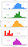 |
Fig. 1 Galaxy type distribution of our sample split by the SN type. The SN type and the number of events are presented at the top of each panel. |
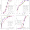 |
Fig. 2 Cumulative distributions of the local M*L, sSFRL, |

3.2 EW and VEL distributions for Na I D
In this section, we explore differences in EW and VEL based only on the SN type. The left panel of Figure 3 shows the measured Na I D EW distribution of our sample. Significant variations in EW are observed across different SN types. Specifically, SNe Ia-pass exhibit the lowest EW values with a median of EW = −0.03 Å (see Table 2), followed by SNe-int (0.15 Å), SNe II (0.23 Å), SNe Ia-SF (0.52 Å), and SE-SNe (0.55 Å). K-S tests comparing these distributions reveal that SNe Ia-pass differ significantly from most other SN types, with the null hypothesis of shared parent population rejected at a confidence level exceeding 50%. This trend aligns with the fact that passive galaxies, where SNe Ia-pass occur, have a substantially lower gas content (Young et al. 2011).
An interesting result is the seemingly low median value of Na I D EWs measured for SNe-int. Taking the mean, however, results in a much higher value of 0.47 Å and from Figure 3 (left panel), we see that the distribution is first full of low values but rapidly increases to very high values, possibly indicating two populations. Although these SNe interact with circumstellar material and have traditionally been associated with very massive progenitors, environmental studies (e.g. Habergham et al. 2014) have shown that SNe-int exhibit a relatively weak association with ongoing star formation, as traced by Hα emission (but see top-right panel of Figure 2 and Table E.1). This weak association might help explain the SNe-int with low Na I D EWs. At the same time, the presence of several high EW values among SNe-int suggests that a sub-set of these objects exhibits significant absorption. Notably, SNe-int also show a higher frequency of negative measured EWs (mostly consistent with zero) compared to other SN types. To test for the impact of this effect, we exclude all SNe with EW+σEW < 0, and repeat the analysis. After applying this cut, the results remain unchanged and no significant differences emerge. This suggests that the observed trend is likely intrinsic rather than an artefact of measurement uncertainties.
A more surprising result from Figure 3 (left panel) is that SNe Ia-SF have a significantly stronger EW distribution than SNe II and actually more so resembles what has been observed for SE-SNe. The EW of SNe Ia-SF and SE-SNe are in fact statistically consistent with being drawn from the same parent distribution. The discrepancy with SNe II is in agreement with the trends identified in Section 3.1, which show that SNe II are in older and less star-forming environments than SE SNe. However, SNe Ia-SF have properties more in line with SNe II (similar local sSFR and slightly older local age), but do have EW measurements of Na I D that are more similar to SE SNe. At first glance, we might suspect that this result is driven by redshift effects, given that SNe Ia are intrinsically brighter and their Na I D features may be easier to detect at larger distances. However, as we are using a redshift-matched bootstrap K-S test (see Section 3 and Paper II, for more details) to ensure that the redshift distributions of the two samples are directly comparable, it is clear that these results are not driven by redshift effects (see Appendix B). Instead, it indicates that the result is robust and likely reflects a genuine physical trend.
To mitigate the known dependence of the strength of the Na I D narrow line with galaxy properties that are, in turn, also correlated with SN types, we normalised the EW measurements by ∆α and M*L, following the analytic correlations found in Paper II (see Appendix C). Therein, we showed that the Na I D EW is moderately correlated with Δα ( ), SFR0L (
 ), AVL (
 ) and M*L (
 ). Subtracting the normalised offset (∆α) relation removes this dependence, but since the SFR0L and AVL also depend on the M*L, we additionally subtracted the M*L relation. The results of this ’normalised’ EW are shown in the right panel of Figure 3. Although visually the cumulative distributions look more separated, the difference according to the K-S statistics for the majority of the comparisons decreased (see Appendix D). This is partly due to the decrease in the number of events, as not all SNe have their local galaxy parameters measurements available. The resulting distributions in CCSNe and SNe Ia-SF start to appear more similar; however, the distribution of SNe Ia-pass differs from these, exhibiting much lower EW values. Statistically, the comparison between SNe Ia-pass and SNe II is the only one that increases, going on to show a stronger difference, namely, from PMC = 67% to PMC = 99%. For SNe Ia-pass and SNe-int, the difference observed before the normalisation disappears, declining from PMC = 51% to PMC = 22%. Visually, the distribution of SNe-int shows more clearly the bi-modality between no and strong Na I D absorption.
Figure 4 shows the Na I D VEL distributions for each SN type. Since the velocities are impossible to measure when the lines are inexistent or very weak, we did not consider objects with |EW| < 0.3Å. We observed strong differences for SNe-int compared to SNe Ia-SF (PMC = 79%) and SE-SNe (PMC = 59%). For the rest of the comparisons, no significant differences were found. Overall, SNe-int exhibit the highest fraction of SNe with blueshifted absorption with a median velocity of VEL = −59 km s−1. The remaining SNe types have a median between −18 and 33 km s−1. This finding suggests that the VEL may be largely independent of the SN type. The stronger blueshifted VEL in the SNe-int sample could be linked to CSM moving towards the observer. However, confirming this interpretation remains challenging due to the large measured uncertainties and the limited number of available observations. Therefore, we carefully investigated potential measurement biases, in particular, contamination from nearby narrow emission or absorption features. A visual inspection of the spectra and the relevant spectral lines supports the reliability of the measured values. In addition, restricting the sample to only positive absorption values (EW > 0.3 Å) produces similar results. Similarly, limiting the sample to measurements with small relative uncertainties (EW/ERR > 3) also provides similar median negative blueshifted lines, indicating that the observed trend is robust against these selection criteria. Alternative explanations beyond a CSM origin may involve nearby dust clouds accelerated towards the observer by SN radiation pressure (Hoang et al. 2019). However, the energy released by SNe-int is comparable to that of SNe Ia, for which no corresponding excess blueshift has been observed. This suggests that radiation-driven dust acceleration alone is unlikely to account for the observed blueshift in the SNe-int sample. Table 2 provides the median, average and median absolute deviation (MAD) for the Na I D VEL.
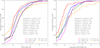 |
Fig. 3 Cumulative distributions of the measured Na I D EW (left) and the EW normalised by the offset and M*L (right) for each SN type. The number of events of each SN type and the results from the K-S test comparing two different populations are also shown in each panel. |
Statistics for the EW and VEL of Na I D for different SN types.
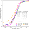 |
Fig. 4 Cumulative distributions of the Na I D VEL divided into the SN type. The number of events of each SN type and the results from the K-S test comparing two different populations are also shown in each panel. |
3.3 EW and VEL distributions for other narrow lines
We also measured the EW and VEL of Ca II H, Ca II K, K I 1, KI 2, DIB-4428, DIB-5780, and DIB-6283. When comparing across different SNe sub-types, we found statistically significant differences for Ca II H, Ca II K, DIB-4428, DIB-6283, and KI2; namely, SNe Ia-pass tend to show the weakest absorption overall (i.e. the lowest EWs), while it is either SE-SN or SNe Ia-SF show the strongest. This is in agreement with our findings for the NaID EW (Section 3.2). Specifically, for CaII H, the most notable differences occur when comparing SNe Ia with other sub-types. The statistical significance of the differences between SNe Ia-pass and other types ranges from 58 to 72%. These differences become more pronounced when comparing SNe Ia-SF to CCSNe, with significance levels between 70 and 90%. In this case, SNe Ia-SF exhibit stronger CaII H EW absorption, while SNe-Ia-pass again show the weakest.
For Ca II K, the EW distributions also reveal strong differences. SNe Ia-pass differ significantly from SE-SNe, SNe II, and SNe Ia-SF (PMC = 94−100%). A moderate difference is also found between SNe Ia-SF and SE-SNe (PMC = 68%). SE-SNe show the highest EW values for this line, while SNe Ia-pass continue to exhibit the lowest values.
When comparing the EW distribution of DIBs, we see notable differences in DIB-6283 and DIB-4458. For DIB-6283, significant differences have been observed between SE-SNe and both SNe Ia-pass (PMC = 80%) and SNe Ia-SF (PMC = 78%), as well as between SNe-int and both SNe Ia-SF (PMC = 95%) and SNe II (PMC = 66%). SNe-int shows the strongest DIB-6283 EW, followed by SE-SNe. For DIB-4458, significant differences are only found between SNe Ia-SF and both SNe-int (PMC = 96%) and SNe-II (PMC = 83%), with SNe Ia-SF showing the highest EW values. Finally, for K I 2, we can observe strong differences between SNe-Ia-SF and both SNe II (PMC = 85%) and SE-SNe (PMC = 62%).
Regarding the VEL distributions, differences are only found for the Ca II lines. For Ca II K, these differences are seen between SNe-int and SNe Ia-SF (PMC = 79%), SE-SNe (PMC = 75%), and SNe Ia-pass (PMC = 57%). For Ca II H, we find a difference between SNe Ia-SF and SNe-int (PMC = 66%). In all cases, SNe-int consistently show the bluest VEL values among the compared groups. No significant VEL differences are detected among SN sub-types for the other lines. Tables E.2 and E.3 (Appendix E) summarise the statistical properties of the narrow absorption lines discussed in this section: Table E.2 reports the K-S statistics for the EW distributions across SN sub-types, while Table E.3 provides the median, average and MAD values.
3.4 Na I D differences based on the SN type and galaxy properties
In Paper II, we showed that the SN EW traces several global and local galaxy properties such as the T-type, the inclination, the galactocentric offset, the local mass, sSFR, age, and dust attenuation. Here we investigate how these properties correlate with our gas indicators when divided by SN type. The K-S statistics and correlations for Na I D EW/VEL distributions for each SN type, divided according to galaxy properties, are presented in Tables E.4-E.8 (Appendix E). The properties with strong K-S test statistics are highlighted in bold, according to their z-matched bootstrap probability of being drawn from different parent populations; namely, probability higher than 50% of a K-S p-value less than 0.05: PMC(p < 0.05) > 50%.
SNe Ia-SF, II, SE, and Int with stronger NaID EWs are generally located in galaxies with higher inclinations, as shown in Paper II, although there are no significant statistical differences when comparing their inclination-split Na I D EW/VEL distributions. Regarding the offsets from the galaxy centres, the trend identified in Paper II persists when separating by SN types. Across all classifications, SNe at lower and higher offsets from the galaxy centre exhibit different Na I D EW distributions. For normalised offsets, the difference is statistically significant for most SN types (PMC > 60%), with weaker Na I D lines found at larger distances from the galaxy centre. This trend is especially pronounced for SNe Ia-SF (PMC = 100%). For the angular and DLR offsets, only SNe Ia (both Ia-pass and Ia-SF) show significant differences in their Na I D EW distributions (PMC > 80%). While a similar trend is seen for CCSNe, the statistical significance is lower. In contrast, we find no significant differences in the VEL distributions across inclination or offset for any SN type.
Regarding the global properties of the SN host galaxies, as for the entire SN sample, we did not find any significant differences in the Na I D EW/VEL distributions. However, the trends observed for local environmental properties do change significantly. The SN types showing the most statistically significant differences are SNe Ia-SF and SE-SNe. For SNe Ia-SF, we found strong differences (PMC ~ 58−99%) in the EW distributions for various parameters, including recent (< 100 Myr) SFR0L (PMC = 99%), sSFR0L (PMC = 78%), AV (PMC = 91%), M*L (PMC = 84%) and tage (PMC = 58%). This indicates that SNe Ia-SF with higher Na I D EW values tend to be located in more massive, actively star-forming, dustier (more attenuated), and younger environments. For SE-SNe, the most significant differences are found with AV (PMC = 100%), SFR0L (PMC = 91%), sSFR0L (PMC = 80%), M*L (PMC = 86%), and the attenuation slope, n (PMC = 78%), suggesting that SE-SNe with higher Na I D EW are associated with dustier, more massive, and actively star-forming galaxies. Although no statistically significant differences are found for the other SN types (SNe Ia-pass, II, Int), similar trends are seen: higher Na I D EWs are typically associated with more massive, star-forming, younger, and dustier environments. This reinforces the conclusions from Paper II, suggesting that the SN Na I D narrow lines better trace the local environment, rather than the global properties of the host galaxies.
4 Discussion
Using over 10 000 spectra from ∼1800 low-redshift SNe of different types (SNe II, SE-SNe, SNe-int, SNe Ia-SF, and SNe Ia-pass), along with their corresponding host galaxy information, we investigated the properties of the host galaxies and how they affect the strength of narrow interstellar absorption lines (especially Na I D ) in SN spectra. In this section, we interpret our key findings presented above and set them in the context of previous studies.
4.1 Comparison to previous SN environmental studies
Studies focusing on SN host galaxies are common and often employ a variety of samples and analytical techniques, offering more detailed insights into the environments of different SN types (see Anderson et al. 2015, and references therein). Using the pixel statistics technique (NCR), Anderson et al. (2012) found that SNe Ic show the strongest association with Hα emission (tracing very young stellar populations), followed by SNe Ib, SNe II and, finally, SNe Ia, which shows the weakest degree of association (also see Anderson & James 2008; Anderson et al. 2015). These results suggest that SNe Ic more closely trace the SF of their host galaxies than SNe II. Galbany et al. (2014) reported similar results when comparing SNe Ia, II and Ibc, but using integral field spectroscopy (IFS) of the hosts. Our analysis supports these previous conclusions; in particular, we find that the sSFR0L of SE-SNe are systematically higher than those from SNe II and SNe Ia (see top-right panel of Figure 2 and Table E.1).
When interacting SNe are included in these NCR studies, the results have been unexpected, suggesting that at least some SNe-int may arise from older populations and lower-mass progenitors (Habergham et al. 2014; Anderson et al. 2015; Kuncarayakti et al. 2018). Despite the limited number of SNe-int in our sample, we observed this trend only at the low-end of the sSFR0L distribution, rapidly increasing to high values, more similar to SE-SNe at the high-end. This could mean that SNe-int may have a mix of progenitors (also see Galbany et al. 2018), although the statistics are too small in scope to draw any firm conclusions.
We reach similar results when analysing the local  . As expected, SNe Ia (both Ia-pass and Ia-SF) are associated with older populations, consistent with long progenitor lifetimes. Among CCSNe, we find a strong difference in the tage distributions between SNe II and SE-SNe (PMC = 99%), providing robust evidence that SE-SNe preferentially occur in significantly younger environments. Interestingly, SNe-int appear to arise from progenitors with intermediate ages, suggesting that they might occupy an evolutionary phase between those of SE-SNe and SNe II.
We also compared our stellar masses, M*, with previous studies. Given that metallicity is a key parameter in stellar evolution, and considering that metallicity (Z⊙) estimates obtained from PROSPECTOR are not fully reliable (see e.g. Duarte et al. 2023), we adopted the M* as a proxy for metallicity. From a theoretical perspective, metallicity-driven mass loss in single-star progenitors predicts that SE-SNe should preferentially occur in more massive, metal-rich environments (e.g. Meynet & Maeder 2005; Eldridge et al. 2008).
Our sample covers a wide range of masses, from relatively low-mass galaxies with log(M*G) ∼ 8 M⊙ to more massive hosts reaching log(M*G) ∼ 12 M⊙. This mass range is comparable to the host galaxy sample analysed by Galbany et al. (2018). Studies including a narrower mass range (e.g. Galbany et al. 2014, log(M*G) ∼ 9−10 M⊙) reported systematic differences across all SN types, with SNe Ia at higher M* and SE-SNe in the lower end. In our data, SNe II and SE-SNe exhibit similar M* distributions (with SNe II tending towards slightly lower masses), both much lower than those of SNe Ia (Ia-SF and Ia-pass). This trend is consistent at both global and local scales. While higher metallicity should, in principle, favour SE-SNe in more massive environments, the inclusion of Type Ic broad-line SNe (SNe Ic-BL), known to occur preferentially at lower metallicities, can broaden and shift the M* distribution, reducing the contrast with SNe II. Nevertheless, the number of SNe Ic-BL in our sample is very small and excluding them does not significantly alter the overall distributions. Therefore, the observed similarity in M* distributions between SNe II and SE-SNe appears to be robust, indicating that metallicity is not the dominant parameter shaping the CCSN diversity (also see Anderson et al. 2012). Instead, other parameters, such as binarity, stellar rotation, or zero-age main sequence (ZAMS) mass are likely to play a more significant role in determining the final SN sub-type. However, to definitively disentangle these effects, direct metallicity indicators (instead of proxies, e.g. stellar mass) for each CCSN sub-type (SNe II, IIb, Ib, Ic, Ic-BL) across large, unbiased samples are essential. While our sample is somewhat biased against the faintest galaxies, our findings highlight the importance of including low-mass hosts to fully capture the diversity of SN progenitor environments.
4.2 Comparison to previous studies analysing narrow lines
Statistical studies focusing on the narrow interstellar lines in SN spectra remain limited. In SNe Ia, these narrow lines have primarily been analysed to investigate and constrain progenitor scenarios (e.g. Maguire et al. 2013; Phillips et al. 2013; Sternberg et al. 2014; Clark et al. 2021). However, analyses directly linking the strength of these narrow lines to galaxy properties are rare. To our knowledge, only two such studies have been published. The first was published by Anderson et al. (2015) explored how the Na I D absorption in SNe II changes with environment, finding that events with detectable Na I D tend to occur closer to the centres of their host galaxies. Our results confirm this trend: SNe II located at smaller offsets exhibit higher EW values, as do all other SN types. A K-S test comparing the EW distributions shows a statistically significant difference, with PMC = 86% (see Table E.6).
The second work, presented by Nugent et al. (2023), analysed a sample of SNe Ia with different ejecta velocities and explored correlation with host galaxy properties. They found no statistically significant difference in the Na I D distributions between high- and low-velocity SNe Ia; however, they noted that high velocity events tend to exhibit higher EWs and are more concentrated near the centre of their host galaxies. Although our current analysis does not split SN Ia based on their expansion velocities, we find that SNe Ia-SF generally have larger Na I D EWs and are more likely to be located in central regions compared to SNe Ia-pass. We also find that when we are dividing the EW measurements by the median of the normalised offset, both SNe Ia-pass and SNe Ia-SF with larger EWs are more frequently located in the central regions of their hosts. The difference between central and outer-region events is statistically significant, with PMC = 71% for SNe Ia-pass and PMC = 99% for SNe Ia-SF. While these findings suggest a connection between line strength and local environment, the possible association between high-velocity SNe Ia and star-forming hosts remains inconclusive. We will address this question in more depth by examining SN Ia sub-populations in a forthcoming study.
4.3 Na I D EW as tracer of local environments
In Paper II, we showed that the narrow absorption lines in SN spectra are effective tracers for statistically probing the ISM properties of host galaxies. Specifically, we found significant differences in Na I D EW when we split the sample by local M*L and local sSFR0L, with higher EW values associated with more massive galaxies and actively SF regions. In this work, we extended that analysis by examining EW distributions per SN type, revealing that SNe Ia-SF and SE-SNe drive the strongest differences. For both types, we identify five environmental parameters that show statistically significant differences, four of which are shared: SFR0L, AVL, M*L, and sSFR0L. Additionally, SNe Ia-SF show a dependence on tage, which can be attributed to the large range of ages observed in SNe Ia, as opposed to CCSNe. SE-SNe also exhibit differences in the n parameter, but this comes from the strong correlation between AV and n (see e.g. Duarte et al. 2023): since SE-SNe are the SN type with the largest Na I D differences with AV (PMC =100%), it is not surprising that n also shows strong p-values. Our results suggest that SNe Ia-SF and SE-SNe with stronger Na I D lines tend to occur in dustier, more massive and more actively starforming environments. This reinforces the idea that the narrow Na I D absorption line is a sensitive tracer of local ISM, providing insight into the immediate environments of SN progenitors for these two SN types.
To better understand why two SN classes originating from very different stellar populations, one typically from older (Ia-SF) and the other from younger (SE-SNe) progenitors, exhibit similar environmental trends with Na I D EW, we investigate deeper into their local host galaxy conditions. For this analysis, we used a Monte Carlo and applied the Fasano-Franceschini (F-F) test (Fasano & Franceschini 1987), a non-parametric, multidimensional generalisation of the K-S test. Using the parameters tage (since SNe Ia-SF and SE-SNe originate from different progenitor populations) together with the local parameters with the strongest differences (M*L, sAVL and sSFR0L)5, we find that the environments of SNe Ia-SF are actually statistically different from those of SE-SNe (pMC-value= 0.009 ± 0.042; PMC =85%). Specifically, SNe Ia-SF tend to explode in more massive environments with lower current SF activity. If we remove M*L from the environmental parameters and we repeat the F-F test, we still find significant environmental differences between SNe Ia-SF and SE-SNe (p-value= 0.014 ± 0.064; PMC =77%).
The apparent similarity in the Na I D distributions of SNe Ia-SF and SE-SNe (K-S test with PMC =10% before normalisation; PMC =18% after normalisation; Figure 3) is in stark contrast with the clearly distinct progenitor environments found according to the multi-dimensional F-F test. This suggests that similar ISM absorption signatures can arise from different environments and perhaps different progenitor scenarios. These scenarios may involve binary interaction, progenitor mass loss, or processes related to the explosion itself. More specifically, the EW behaviour could originate from the presence of more nearby material around the explosion site, either (a) from CSM ejected by the progenitor system before the explosion or (b) through interaction of the SN radiation with patchy ISM material in the immediate vicinity.
A fraction of SNe Ia exhibit Na I D absorption in excess of what would be expected based on their AV values inferred from light curves (Phillips et al. 2013; Maguire et al. 2013). One interpretation is that this additional absorption originates from CSM associated with the progenitor system. Alternatively, intense SN radiation can affect nearby dust clouds by inducing cloud-cloud collisions (Hoang 2017) or imprinting centrifugal forces on dust grains through radiative torques, leading to their disruption (Hoang et al. 2019; Giang et al. 2020). Such processes can release metals previously locked in dust grains, increasing the fraction of free sodium atoms in the local environment. The strength of this effect depends on the intensity of the SN radiation and the proximity of the dust clouds. Since SNe Ia are generally more energetic than CCSNe, such scenarios could partially explain the higher abundance of sodium in SNe Ia-SF without the need for CSM.
5 Conclusions
In this paper, we have analysed the narrow interstellar lines in SNe spectra and investigated their connection to both local and global properties of the host galaxies. Our analysis combines the EW and VEL measurements presented in Paper I for over 1800 SNe, with the host galaxy properties characterised in Paper II. Our main results are as follows.
CCSNe occur at a non-negligible number in early-type galaxies, in agreement with previous studies. Clear host differences emerge among SN types: SNe Ia-pass occur in older, more massive, and less dusty systems; whereas SNe Ia-SF are found in more massive but dustier hosts, resembling CCSNe. Consistently, SNe II and SE-SNe show the highest specific attenuation, both globally and locally.
SE-SNe display the highest local sSFR, reinforcing their association with more massive progenitors. In contrast, SNe-int occupy an intermediate regime in both age and sSFR, suggesting a mixed origin between SE-SNe and SNe II progenitor populations.
SNe Ia in passive galaxies exhibit significantly weaker narrow absorption features compared to CC-SNe and SNe Ia-SF, suggesting lower interstellar gas content in quiescent environments.
The Na I D EW distribution of SNe II is much lower than that of both SNe Ia-SF and SE-SNe, which is unexpected given their association with SF regions and deeper galactic locations. This could indicate that absorption (for SESN and SNe Ia-SF) might include more nearby material beyond the line-of-sight ISM.
The similarity between SNe Ia-SF and SE-SNe Na I D EW distributions, despite their different environment, suggests that different progenitors and environments can produce a comparable level of absorption, possibly through CSM expelled prior to explosion or SN interactions with patchy ISM clouds.
Across all measured narrow interstellar lines (Na I D, Ca IIH, Ca IIK, DIB-4428, DIB-5780, DIB-6283, KI 1, and KI 2), SNe Ia-pass consistently display the weakest EWs, while it is either SE-SN or SNe Ia-SF that display the strongest.
Detailed analyses focused on specific SN types will be presented in forthcoming papers. These studies will particularly explore how SN spectral and photometric properties are correlated with host galaxy characteristics and the strength of narrow interstellar absorption features. The goal is to disentangle the physical mechanisms behind the observed diversity among SN sub-types and to improve the constraints set on progenitor scenarios using environmental diagnostics.
Acknowledgements
We thank the anonymous referee for the comments and suggestions that have helped us to improve the paper. C.P.G. acknowledges financial support from the Secretary of Universities and Research (Government of Catalonia) and by the Horizon 2020 Research and Innovation Programme of the European Union under the Marie Sklodowska-Curie and the Beatriu de Pinós 2021 BP 00168 programme. C.P.G. and L.G. recognise the support from the Spanish Ministerio de Ciencia e Innovación (MCIN) and the Agencia Estatal de Investigación (AEI) 10.13039/501100011033 under the PID2023-151307NB-I00 SNNEXT project, from Centro Superior de Investigaciones Científicas (CSIC) under the PIE project 20215AT016 and the program Unidad de Excelencia María de Maeztu CEX2020-001058-M, and from the Departament de Recerca i Uni-versitats de la Generalitat de Catalunya through the 2021-SGR-01270 grant. We acknowledge the financial support from the María de Maeztu Thematic Core at ICE-CSIC. S.G.G thanks the ESO Scientific Visitor Programme. This research has made use of the PYTHON packages ASTROPY (Astropy Collaboration 2013, 2018, 2022), NUMPY (Harris et al. 2020), MATPLOTLIB (Hunter 2007), SCIPY (Virtanen et al. 2020), pandas (The pandas development team 2020; Wes McKinney 2010).
References
- Anderson, J. P., & James, P. A. 2008, MNRAS, 390, 1527 [NASA ADS] [Google Scholar]
- Anderson, J. P., Habergham, S. M., James, P. A., & Hamuy, M. 2012, MNRAS, 424, 1372 [NASA ADS] [CrossRef] [Google Scholar]
- Anderson, J. P., James, P. A., Habergham, S. M., Galbany, L., & Kuncarayakti, H. 2015, PASA, 32, e019 [NASA ADS] [CrossRef] [Google Scholar]
- Arcavi, I., Gal-Yam, A., Kasliwal, M. M., et al. 2010, ApJ, 721, 777 [NASA ADS] [CrossRef] [Google Scholar]
- Astropy Collaboration (Robitaille, T. P., et al.) 2013, A&A, 558, A33 [NASA ADS] [CrossRef] [EDP Sciences] [Google Scholar]
- Astropy Collaboration (Price-Whelan, A. M., et al.) 2018, AJ, 156, 123 [Google Scholar]
- Astropy Collaboration (Price-Whelan, A. M., et al.) 2022, ApJ, 935, 167 [NASA ADS] [CrossRef] [Google Scholar]
- Bersten, M. C., Benvenuto, O., & Hamuy, M. 2011, ApJ, 729, 61 [NASA ADS] [CrossRef] [Google Scholar]
- Bersten, M. C., Benvenuto, O. G., Nomoto, K., et al. 2012, ApJ, 757, 31 [Google Scholar]
- Clark, P., Maguire, K., Bulla, M., et al. 2021, MNRAS, 507, 4367 [NASA ADS] [CrossRef] [Google Scholar]
- Dessart, L., Hillier, D. J., Waldman, R., & Livne, E. 2013, MNRAS, 433, 1745 [NASA ADS] [CrossRef] [Google Scholar]
- Dessart, L., Hillier, D. J., Woosley, S. E., & Kuncarayakti, H. 2023, A&A, 677, A7 [Google Scholar]
- Dessart, L., Gutiérrez, C. P., Ercolino, A., Jin, H., & Langer, N. 2024, A&A, 685, A169 [NASA ADS] [CrossRef] [EDP Sciences] [Google Scholar]
- Duarte, J., González-Gaitán, S., Mour$äo, A., et al. 2023, A&A, 680, A56 [NASA ADS] [CrossRef] [EDP Sciences] [Google Scholar]
- Duarte, J., González-Gaitán, S., Mour$äo, A., et al. 2025, A&A, 700, A169 [NASA ADS] [CrossRef] [EDP Sciences] [Google Scholar]
- Eldridge, J. J., Izzard, R. G., & Tout, C. A. 2008, MNRAS, 384, 1109 [Google Scholar]
- Fasano, G., & Franceschini, A. 1987, MNRAS, 225, 155 [NASA ADS] [CrossRef] [Google Scholar]
- Folatelli, G., Van Dyk, S. D., Kuncarayakti, H., et al. 2016, ApJ, 825, L22 [NASA ADS] [CrossRef] [Google Scholar]
- Galbany, L., Anderson, J. P., Rosales-Ortega, F. F., et al. 2016, MNRAS, 455, 4087 [NASA ADS] [CrossRef] [Google Scholar]
- Galbany, L., Anderson, J. P., Sánchez, S. F., et al. 2018, ApJ, 855, 107 [Google Scholar]
- Galbany, L., Stanishev, V., Mour$äo, A. M., et al. 2014, A&A, 572, A38 [NASA ADS] [CrossRef] [EDP Sciences] [Google Scholar]
- Garn, T., & Best, P. N. 2010, MNRAS, 409, 421 [Google Scholar]
- Giang, N. C., Hoang, T., & Tram, L. N. 2020, ApJ, 888, 93 [NASA ADS] [CrossRef] [Google Scholar]
- Gomes, J. M., Papaderos, P., Vílchez, J. M., et al. 2016, A&A, 585, A92 [NASA ADS] [CrossRef] [EDP Sciences] [Google Scholar]
- González-Gaitán, S., Gutiérrez, C. P., Anderson, J. P., et al. 2024, A&A, 687, A108 [NASA ADS] [CrossRef] [EDP Sciences] [Google Scholar]
- González-Gaitán, S., Gutiérrez, C. P., Martins, G., et al. 2025, A&A, 700, A119 [NASA ADS] [CrossRef] [EDP Sciences] [Google Scholar]
- Gutiérrez, C. P., González-Gaitán, S., Folatelli, G., et al. 2016, A&A, 590, A5 [Google Scholar]
- Gutiérrez, C. P., Sullivan, M., Martinez, L., et al. 2020, MNRAS, 496, 95 [CrossRef] [Google Scholar]
- Gutiérrez, C. P., Bersten, M. C., Orellana, M., et al. 2021, MNRAS, 504, 4907 [CrossRef] [Google Scholar]
- Gutiérrez, C. P., Pastorello, A., Bersten, M., et al. 2022, MNRAS, 517, 2056 [CrossRef] [Google Scholar]
- Habergham, S. M., Anderson, J. P., James, P. A., & Lyman, J. D. 2014, MNRAS, 441, 2230 [CrossRef] [Google Scholar]
- Hakobyan, A. A., Petrosian, A. R., McLean, B., et al. 2008, A&A, 488, 523 [NASA ADS] [CrossRef] [EDP Sciences] [Google Scholar]
- Harris, C. R., Millman, K. J., van der Walt, S. J., et al. 2020, Nature, 585, 357 [NASA ADS] [CrossRef] [Google Scholar]
- Hillier, D. J., & Dessart, L. 2019, A&A, 631, A8 [NASA ADS] [CrossRef] [EDP Sciences] [Google Scholar]
- Hoang, T. 2017, ApJ, 836, 13 [Google Scholar]
- Hoang, T., Tram, L. N., Lee, H., & Ahn, S.-H. 2019, Nat. Astron., 3, 766 [Google Scholar]
- Hunter, J. D. 2007, Comp. Sci. Eng., 9, 90 [NASA ADS] [CrossRef] [Google Scholar]
- Irani, I., Prentice, S. J., Schulze, S., et al. 2022, ApJ, 927, 10 [Google Scholar]
- Jerkstrand, A., Fransson, C., Maguire, K., et al. 2012, A&A, 546, A28 [NASA ADS] [CrossRef] [EDP Sciences] [Google Scholar]
- Johnson, B. D., Leja, J., Conroy, C., & Speagle, J. S. 2021, ApJS, 254, 22 [NASA ADS] [CrossRef] [Google Scholar]
- Kolmogorov, A. N. 1933, Giorn Dell’inst Ital Degli Att, 4, 89 [Google Scholar]
- Kozyreva, A., Gilmer, M., Hirschi, R., et al. 2017, MNRAS, 464, 2854 [NASA ADS] [CrossRef] [Google Scholar]
- Kuncarayakti, H., Doi, M., Aldering, G., et al. 2013, AJ, 146, 31 [NASA ADS] [CrossRef] [Google Scholar]
- Kuncarayakti, H., Anderson, J. P., Galbany, L., et al. 2018, A&A, 613, A35 [NASA ADS] [CrossRef] [EDP Sciences] [Google Scholar]
- Leja, J., Johnson, B. D., Conroy, C., van Dokkum, P. G., & Byler, N. 2017, ApJ, 837, 170 [NASA ADS] [CrossRef] [Google Scholar]
- Maguire, K., Sullivan, M., Patat, F., et al. 2013, MNRAS, 436, 222 [CrossRef] [Google Scholar]
- Martinez, L., Bersten, M. C., Anderson, J. P., et al. 2022, A&A, 660, A41 [NASA ADS] [CrossRef] [EDP Sciences] [Google Scholar]
- Mattila, S., Smartt, S. J., Eldridge, J. J., et al. 2008, ApJ, 688, L91 [NASA ADS] [CrossRef] [Google Scholar]
- Mazzali, P. A., Benetti, S., Stehle, M., et al. 2005, MNRAS, 357, 200 [NASA ADS] [CrossRef] [Google Scholar]
- Meynet, G., & Maeder, A. 2005, A&A, 429, 581 [CrossRef] [EDP Sciences] [Google Scholar]
- Moriya, T. J., Subrayan, B. M., Milisavljevic, D., & Blinnikov, S. I. 2023, PASJ, 75, 634 [NASA ADS] [CrossRef] [Google Scholar]
- Morozova, V., Piro, A. L., Renzo, M., et al. 2015, ApJ, 814, 63 [Google Scholar]
- Müller-Bravo, T., & Galbany, L. 2022, J. Open Source Softw., 7, 4508 [CrossRef] [Google Scholar]
- Nugent, A. E., Polin, A. E., & Nugent, P E. 2023, arXiv e-prints [arXiv:2304.10601] [Google Scholar]
- Pessi, T., Anderson, J. P., Lyman, J. D., et al. 2023, ApJ, 955, L29 [Google Scholar]
- Phillips, M. M., et al. 2013, ApJ, 779, 38 [NASA ADS] [CrossRef] [Google Scholar]
- Schawinski, K., Kaviraj, S., Khochfar, S., et al. 2007, ApJS, 173, 512 [NASA ADS] [CrossRef] [Google Scholar]
- Sedgwick, T. M., Baldry, I. K., James, P. A., Kaviraj, S., & Martin, G. 2021, arXiv e-prints [arXiv:2106.13812] [Google Scholar]
- Smartt, S. J., Eldridge, J. J., Crockett, R. M., & Maund, J. R. 2009, MNRAS, 395, 1409 [CrossRef] [Google Scholar]
- Smirnov, N. V. 1939, Bull. Math. Univ. Moscou, 2, 3 [Google Scholar]
- Spearman, C. 1904, Am. J. Psychol., 15, 201 [CrossRef] [Google Scholar]
- Sternberg, A., Gal-Yam, A., Simon, J. D., et al. 2011, Science, 333, 856 [NASA ADS] [CrossRef] [Google Scholar]
- Sternberg, A., Gal-Yam, A., Simon, J. D., et al. 2014, MNRAS, 443, 1849 [NASA ADS] [CrossRef] [Google Scholar]
- The pandas development team 2020, https://doi.org/10.5281/zenodo.3509134 [Google Scholar]
- Turatto, M., Benetti, S., & Cappellaro, E. 2003, in From Twilight to Highlight: The Physics of Supernovae, eds. W. Hillebrandt, & B. Leibundgut (Berlin: Springer), 200 [Google Scholar]
- Van Dyk, S. D. 2017, Phil. Trans. R. Soc. London Ser. A, 375, 20160277 [Google Scholar]
- Van Dyk, S. D., Garnavich, P. M., Filippenko, A. V., et al. 2002, PASP, 114, 1322 [NASA ADS] [CrossRef] [Google Scholar]
- Van Dyk, S. D., Li, W., & Filippenko, A. V. 2003, PASP, 115, 1289 [NASA ADS] [CrossRef] [Google Scholar]
- Virtanen, P., Gommers, R., Oliphant, T. E., et al. 2020, Nat. Methods, 17, 261 [Google Scholar]
- Vogl, C., Sim, S. A., Noebauer, U. M., Kerzendorf, W. E., & Hillebrandt, W. 2019, A&A, 621, A29 [NASA ADS] [CrossRef] [EDP Sciences] [Google Scholar]
- Wes McKinney 2010, in Proceedings of the 9th Python in Science Conference, eds. Stéfan van der Walt, & Jarrod Millman, 56 [Google Scholar]
- Young, L. M., Bendo, G. J., & Lucero, D. M. 2009, AJ, 137, 3053 [Google Scholar]
- Young, L. M., Bureau, M., Davis, T. A., et al. 2011, MNRAS, 414, 940 [NASA ADS] [CrossRef] [Google Scholar]
- Zahid, H. J., Yates, R. M., Kewley, L. J., & Kudritzki, R. P. 2013, ApJ, 763, 92 [NASA ADS] [CrossRef] [Google Scholar]
Since SFR0L, AVL show strong dependency on the M*L, we adopted the normalised quantities sAVL and sSFR0L to account for this effect.
Appendix A Specific attenuation
In this work, we introduce the term specific attenuation (sAV) to refer to the attenuation (AV) normalised by stellar mass (M*). Attenuation is strongly correlated with stellar mass because more massive galaxies generally contain more dust. This is due to a larger fraction of stars enriching the ISM with metals, which are needed to form dust grains, as well as the greater gravitational potential retaining the dust. As a result, these galaxies naturally exhibit higher attenuation values. Without normalisation, observed trends in AV could simply mirror underlying trends in M*, which itself correlates with various galaxy properties such as metallicity, SFR, age, and even scattering (Duarte et al. 2025).
Figure A.1 shows the AV distributions before normalisation, while the lower right panel of Figure 2 shows the normalised AV values (i.e. sAv). This normalisation accounts for the intrinsic scaling between mass and dust content, allowing us to isolate dustiness relative to galaxy mass. By examining sAV, we can better assess how dust properties vary across different SN host environments independently of galaxy mass. For example, a high sAV indicates a galaxy that is unusually dusty for its mass, which may reflect more active SF or denser ISM conditions. Conversely, low sAV values suggest relatively dust-poor environments, often associated with more quiescent galaxies. Thus, specific attenuation provides a more refined understanding of the dust environments where different SN progenitors arise.
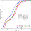 |
Fig. A.1 Cumulative distributions of the local M*L for different SN types. The number of events of each SN type and the results from the K-S test comparing two different populations are also shown in each panel. |
Appendix B Redshift effects
Figure B.1 shows the cumulative distributions of the measured Na I D EW or each SN type (same as Figure 3) but restricted to a sub-sample of events with z < 0.05. A comparison between Figures 3 and B.1 shows that the distributions remain largely unchanged, indicating that the results are not driven by redshift effects.
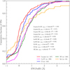 |
Fig. B.1 Cumulative distributions of the measured Na I D EW for a sub-sample of events restricted to z < 0.05. |
Appendix C Normalised Na I D EW
In Paper II, we identified a dependence of the strength of the Na I D narrow line on Δα, SFR0L and M*L. For galaxy offset, Na I D EW shows an exponential decline with increasing radius. To quantify this behaviour, we computed the rolling median of EW as a function of the normalised offset. We then removed this radial dependence by subtracting from each EW measurement the value predicted by the rolling median at its corresponding offset. This normalisation effectively isolates intrinsic EW variations that are independent of radial position within the galaxy. Normalising by offset removes nearly all correlations. However, because M*L also influence SFR0L and AVL, we applied an analogous correction using M*L. The resulting Na I D EW distributions before and after the normalisations are shown in Figure 3.
Appendix D Down-sampling affects
To evaluate the impact of reducing the number of events in the K-S tests, we applied a random down-sampling procedure to the dataset used in the left panel of Figure 3, matching the sample sizes shown in the right panel of the same figure. Specifically, the original samples (Ia-pass= 139, Ia-SF= 307, II= 174, SE= 174, Int= 85) were randomly down-sampled to the sizes of the corresponding smaller samples (Ia-pass= 50, Ia-SF= 145, II= 100, SE= 91, Int= 23). For each SN type, objects were selected at random and without repetition. This approach preserves the overall shape of the original distributions while mitigating potential biases caused by reducing sample sizes. To account for the intrinsic randomness of the down-sampling procedure, we repeated the process using a Monte Carlo approach with 1000 realisations. The resulting distributions are shown in Figure D.1, together with the original results (left panel). As shown in the figure, the differences between SN types are generally observed after downsampling. In particular, the p-values systematically increase while the corresponding probabilities PMC decrease, indicating a reduced statistical significance when controlling for sample size effects. Table D.1 presents the p-values and PMC obtained from the original distributions, two representative down-sampling realisations, and the median values derived from the 1000 Monte Carlo realisations.
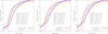 |
Fig. D.1 Cumulative distributions of the measured Na I D EW for the full sample (left) and for two independent realisations obtained after applying the random down-sampling procedure (middle and right panels) for each SN type. The number of events of each SN type and the results from the K-S test comparing two different populations are also shown in each panel. |
K-S statistics comparisons.
Appendix E Supplementary tables
K-S statistics for various properties divided according to SN type.
K-S statistics for EW of several absorption lines divided according to SN type.
Median and MAD of the EW of several narrow lines for different SN types.
K-S statistics and correlations for Na I D EW and VEL in SNe Ia-pass divided according to galaxy properties.
K-S statistics and correlations for Na I DEW and VEL in SNe Ia-SF divided according to galaxy properties.
K-S statistics and correlations for Na I DEW and VEL in SNe II divided according to galaxy properties.
K-S statistics and correlations for Na I DEW and VEL in SE-SNe divided according to galaxy properties.
K-S statistics and correlations for Na I DEW and VEL in SNe-Int divided according to galaxy properties.
All Tables
K-S statistics for EW of several absorption lines divided according to SN type.
K-S statistics and correlations for Na I D EW and VEL in SNe Ia-pass divided according to galaxy properties.
K-S statistics and correlations for Na I DEW and VEL in SNe Ia-SF divided according to galaxy properties.
K-S statistics and correlations for Na I DEW and VEL in SNe II divided according to galaxy properties.
K-S statistics and correlations for Na I DEW and VEL in SE-SNe divided according to galaxy properties.
K-S statistics and correlations for Na I DEW and VEL in SNe-Int divided according to galaxy properties.
All Figures
|
Fig. 1 Galaxy type distribution of our sample split by the SN type. The SN type and the number of events are presented at the top of each panel. |
| In the text | |
|
Fig. 2 Cumulative distributions of the local M*L, sSFRL, |
| In the text | |
|
Fig. 3 Cumulative distributions of the measured Na I D EW (left) and the EW normalised by the offset and M*L (right) for each SN type. The number of events of each SN type and the results from the K-S test comparing two different populations are also shown in each panel. |
| In the text | |
|
Fig. 4 Cumulative distributions of the Na I D VEL divided into the SN type. The number of events of each SN type and the results from the K-S test comparing two different populations are also shown in each panel. |
| In the text | |
|
Fig. A.1 Cumulative distributions of the local M*L for different SN types. The number of events of each SN type and the results from the K-S test comparing two different populations are also shown in each panel. |
| In the text | |
|
Fig. B.1 Cumulative distributions of the measured Na I D EW for a sub-sample of events restricted to z < 0.05. |
| In the text | |
|
Fig. D.1 Cumulative distributions of the measured Na I D EW for the full sample (left) and for two independent realisations obtained after applying the random down-sampling procedure (middle and right panels) for each SN type. The number of events of each SN type and the results from the K-S test comparing two different populations are also shown in each panel. |
| In the text | |
Current usage metrics show cumulative count of Article Views (full-text article views including HTML views, PDF and ePub downloads, according to the available data) and Abstracts Views on Vision4Press platform.
Data correspond to usage on the plateform after 2015. The current usage metrics is available 48-96 hours after online publication and is updated daily on week days.
Initial download of the metrics may take a while.