| Issue |
A&A
Volume 707, March 2026
|
|
|---|---|---|
| Article Number | A215 | |
| Number of page(s) | 9 | |
| Section | Astrophysical processes | |
| DOI | https://doi.org/10.1051/0004-6361/202558230 | |
| Published online | 09 March 2026 | |
The formation of periodic three-body orbits for Newtonian systems
1
Leiden Observatory, Leiden University PO Box 9513 2300 RA Leiden, The Netherlands
2
Mathematisch instituut, Leiden University PO Box 9513 2300 RA Leiden, The Netherlands
3
Niels Bohr International Academy, University of Copenhagen Copenhagen, Denmark
★ Corresponding author.
Received:
24
November
2025
Accepted:
28
January
2026
Abstract
Context. Braids are periodic solutions to the general N-body problem in gravitational dynamics. These solutions seem special and unique but may result from rather usual encounters between four bodies.
Aims. We attempted to learn more about the existence of braids in the Galaxy by reverse engineering the interactions in which they formed.
Methods. We carried out simulations of self-gravitating systems of N particles using fourth-order integration. We started by constructing the specific braid and subsequently bombard it with a single object. We subsequently studied how frequently the bombarded braid dissolves into four singles, a triple and a single, a binary and two singles, or two binaries. The relative proportion of these events gives us insight into how easy it is to generate a braid through the reverse process.
Results. Braids are relatively easily generated from encounters between two binaries or between a triple and a single object, so long as they meet each other, independent of the braid’s stability. We find that three of the explored braids are long-lived and linearly stable against small perturbations, whereas the fourth is unstable and short-lived. The shortest-lived braid appears to be the least stable and the most chaotic. Nonplanar encounters can also lead to braid formation, which, in our experiments, are themselves planar. The parameter space in azimuth and polar angle that leads to braid formation via binary–binary or triple–single encounters is anisotropic, and the distribution has a low fractal dimension.
Conclusions. Since ∼9% of our calculations lead to periodic three-body systems, a substantial fraction, braids may be more common than currently assumed. They could easily temporarily exist as a result of multi-body (binary–binary or triple–single) interactions. We do not expect many stable braids to exist for an extensive period of time, but they may be quite common as transients, surviving for tens to hundreds of periodic orbits. We argue that braids are particularly common in relatively shallow-potential background fields, such as the Oort cloud or the Galactic halo. The formation of braids, however, easily leads to collisions between two or more of their constituents. If composed of compact objects, they potentially form interesting targets for gravitational wave detectors.
Key words: methods: numerical / planets and satellites: dynamical evolution and stability
None of the authors could have done this work without the other two.
© The Authors 2026
 Open Access article, published by EDP Sciences, under the terms of the Creative Commons Attribution License (https://creativecommons.org/licenses/by/4.0), which permits unrestricted use, distribution, and reproduction in any medium, provided the original work is properly cited.
This article is published in open access under the Subscribe to Open model. This email address is being protected from spambots. You need JavaScript enabled to view it. to support open access publication.
1. Introduction
The gravitational N-body problem originated when Newton presented his theory of gravity (Newton 1687). Newton was able to analytically calculate periodic solutions of the two-body problem, which we call “Kepler orbits” (Kepler 1609): two objects in a periodic bound orbit in an elliptical trajectory around their common center of mass. For N > 2, periodic solutions exist, but they are hard to find.
Negative total energy alone cannot be used to determine the long-term stability of a ≥3 body problem because the system is chaotic and therefore evolves in finite time to the ejection of one object, leaving the other two bound in a pair (Poincaré 1891). Euler and Lagrange, however, found potentially long-lived periodic solutions to the three-body problem (see also Henon 1976). These choreographies were later identified as belonging to the same family of periodic solutions (Montgomery 1998). Although so far periodic solutions have been shown to be possibly long-term-stable, there is no theorem to prove this (Terracini 2022).
More than a century later, Moore (1993) proposed a topological classification as a tool for extending the “symbolic dynamics” approach to many-body dynamics. He described the Figure-8 solution (not to be confused with our Fig. 8, which shows the initial azimuth and polar angle distribution for successful braid formation) of the gravitational N-body problem as a braid. Braids are periodic, reducible, and pseudo-Anosov orbits of the gravitational N-body problem (Kajihara et al. 2023). Such a braid emerges when you add the same velocity vector to each of the bodies. In the reference frame, all bodies now travel as parallel strands through time while each strand traces an orbit projected onto one spatial coordinate in time, creating a braid. The form of the Figure-8 then becomes (b1b2−1)3, where bi corresponds to the crossing of the i-th strand over the (i + 1)st (Moore 1993). The stability of such primitive braids was further studied by Simó (1994), who argued that some have relative equilibrium solutions. In astronomical terms, we would describe a braid as a nonhierarchical periodic solution of the N-body problem.
Simó (2001) made the distinction between linearly “stable” and “unstable” choreographies. Of the 18 tested, he found that only the Figure-8 is stable. This finding is consistent with that of Schubart (1956).
Chenciner et al. (2002) made a distinction between the simple choreography of the N-body problem, the definition of which is “a periodic solution in which all N masses trace the same curve without colliding,” and the choreography of arbitrary complexity or symmetry. Both types of choreography exist (Chenciner et al. 2002), although their stability and frequency remain uncertain (Simó 2002). Kapela & Simó (2007) continued this work by studying the stability of complex (asymmetric) braids composed of seven bodies. They found that such a choreography can be dynamically stable.
The astro-dynamical community became aware of the work on braids through the discussion by Chenciner & Montgomery (2000), who further addressed the Figure-8 periodic solution. They, however, did not provide proof for the Figure-8’s long-term stability. Such proof was provided in Kapela & Simó (2007), who demonstrated the linear stability of the Figure-8 orbit.
In the years since, many new braids of various types have been found. Nowadays, most braids are discovered using supercomputers. Li et al. (2018) found 1223 new solutions, which were later expanded with another 13 315 by Li et al. (2021). We conjecture that there exist an infinite number of possible (distinct) periodic solutions to the general N-body problem. Only a subset are expected to be stable against small perturbations, but even so we still expect an infinite number of stable periodic orbits.
Although Li et al. (2021) assert that these braids are stable, it is not a priori clear to what degree they are long-term-stable. The lack of stable braids does not necessarily mean that they do not exist in the Universe but rather that it may be nontrivial to recognize them. We followed up on the work of Heggie (2000), who considered the possibility that Figure-8 braids form from two encountering pairs of objects. In this case, objects could be black holes, stars, planets, planetesimals, or any set of massive objects.
For our calculations, we adopted Newton’s equations of motion with point masses and integrated using a fourth-order numerical scheme. This poses some limitations to the interpretation of our results, as astronomical objects tend to have properties that cause them to interact non-Newtonianly, such as finite radii, orbits affected by general relativistic effects, and radiation pressure1. The effect of numerical errors, and the accuracy in relation to the chaotic dynamics, is discussed in Sect. 4.7.
2. Initial conditions and model parameters
2.1. Initial conditions
We adopted a similar approach as proposed in Heggie (2000), by integrating a three-body braid and bombarding it with a fourth particle. Since Newton’s equations of motion are time symmetric, the inverse interaction then results in a braid, while the original bomb escapes. Heggie (2000) used this strategy to explain how the Figure-8 braid can form from two interacting binaries. We took a more general approach, covering a larger part of the initial parameter space. In the main part of our study, we reduced the initial parameter space by limiting ourselves to interactions in the x − y plane, setting the z coordinate and the velocity perpendicular to the plane equal to zero (note that it is not known if nonplanar braids exist). We further fixed the braid’s orbital phase and orientation but allowed the incoming object to come from any azimuthal direction θ. We randomized in this direction. We relax the assumption on planar encounters in Sect. 4.5, where we discuss the anisotropy of the initial parameter space.
2.2. Parametrics
Once the braid (see Fig. 1) is specified, the mass m4, velocity v4, impact parameter d, and initial distance r of the incoming fourth object remain free to vary. For initial conditions we then have v4(t = 0)≡vin, m4(t = 0)≡min, and d4(t = 0)≡din. Note that if the velocity at infinity satisfies vin = 0, the impact parameter din becomes meaningless. Here units are dimensionless, adopting N-body units following Henon-Heggie, i.e., G = 1 (Heggie & Mathieu 1986).
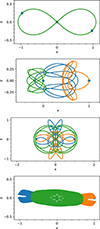 |
Fig. 1. The four three-body braids adopted in this study: the classic Figure-8 problem (top) and three more complicated braids, the unequal-mass problem, I.A.4i.c.(0.5), and |


Simulations were continued until one object (or the center of mass of a binary or triple) satisfied the following conditions: it is farther than 1000 N-body units from the center of mass of the four-body system and is receding from the system with a velocity exceeding the escape speed. It is worth noting that the braid can formally be unbound if an incoming object’s kinetic energy exceeds the braid’s binding energy. For the braids in our experiments, this is the case if the incoming object has mass min = 1 with velocity vin ≳ 1.7. An incoming object with even higher velocity can unbind the braid into four single objects. Unbinding the braid, however, requires efficient energy transfer from the incoming object to the particles in the braid, which is not common (see Table 2). Table 2 also lists the total number of calculations performed, and the fractions of the various resulting configurations.
2.3. Classifying braids
Apart from the Figure-8 braid, we studied two more complex braids, referred to in Li et al. (2018) as I.A.4i.c.(0.5), and  . These names stand for the class of braid, with in parentheses the mass of the third particle (m3) assuming m1 = m2 = 1. The initial conditions for these braids can be written as follows: r1 = (−1,0) = −r2. v1 = (ξa,ξb) = −v2. Here ri ≡ Ixi,yi) is the two-dimensional Cartesian position vector, and equivalently for vi. The two scalars ξa, and ξb, characterize the interaction. For the incoming third particle r3 = (0,0), and v3 = (2ξ1/m3,−2ξ2/m3). All z coordinates and velocities vz are zero (but see Sect. 4.5).
We included a fourth braid with unequal masses, m1 = 0.87, m2 = 0.80, and m3 = 1, which is presented in Table 1 of Li et al. (2021). The initial conditions for the braids we explored are presented in Table 1.
3. Numerical integration
We performed the numerical integration using the Astrophysics Multipurpose Software Environment (AMUSE; Portegies Zwart et al. 2009; Portegies Zwart & McMillan 2018) with the direct fourth-order Hermite predictor-corrector N-body solver Ph4 (McMillan et al. 2012; Portegies Zwart et al. 2022). The calculations are performed using point masses with a time-step parameter of η = 0.01, and zero softening. In Fig. 1 we illustrate the braids integrated for one orbit, and in Sect. 4.7 we discuss the effect of numerical precision on the results.
In Fig. 2 we present I.A.4i.c.(0.5) after 100 N-body time units. By this time, the orbit cannot be classified as a braid; the orbit is not periodic. In the next few hundred time units, one of the three particles is ejected, leaving the other two orbiting their joined center of mass.
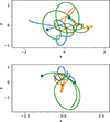 |
Fig. 2. Two representations of braid I.A.4i.c.(0.5) after 100 time units. Top: Unperturbed solution integrated for ten N-body time units. Bottom: Result of the perturbed solution in the same time frame. The introduced perturbation was 10−5 in the x coordinate. Both solutions have clearly deviated from the original braid, and from each other. By this time, the phase space distance between the two solutions is on the order of unity. The orbits are unstable, and in the next 100 crossing times, one particle is ejected. |
Figure 3 shows a distinctly different evolution for model A (the unequal-mass braid case) after 106 time units. By this time, the orbit is still stable, and the orbital shape is indistinguishable from the original orbit, except that it has been subject to precession. We integrated the orbit twice, once with a perturbation of 10−5 to one of the particle’s x-coordinates. However, upon optical inspection, the two orbits are still indistinguishable after integrating for t = 106.
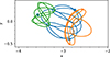 |
Fig. 3. Braid model A after 106 N-body time units. By this time, an initial perturbation of 10−5 has grown to O(10−2). The braid still resembles the original, but the entire orbit has been precessing. |
4. Results
4.1. Braid stability
We determined the stability of a braid by integrating it twice, once with the canonical initial realization (see Table 1) and once with a small perturbation by translating one particle 10−5 along the x-axis. Both integrations were continued for 105 N-body time units, and we determined the Lyapunov timescale by fitting a straight line to the logarithm of the geometric distance evolution in time. The results are presented in Table 2.
The four braids used in this study.
Integration result for the various braids.
The phase-space distance of an initially introduced perturbation in I.A.4i.c.(0.5) grows exponentially, as one would expect for a chaotic system. The Lyapunov timescale for this braid is ∼13 orbits. The other models, Figure-8, model A, and braid  , are linearly stable against infinitesimal perturbations. Note that for braid
  tstable ≳ 9 ⋅ 104 (see Table 2), which strictly speaking does not make it linearly stable, but the accumulation errors in our numerical integration may drive the system’s instability here. Such numerical errors can be mitigated by integrating the braid using arbitrary precision arithmetic, as is explored in Boekholt & Portegies Zwart (2015), which is beyond this papers’ scope.
Interestingly enough, the growth for model A makes periodic excursions, to shrink to values comparable to the initially introduced perturbation (10−5). The timescale of these excursions is about ∼3850 time units, or 642 orbits. This curious behavior can be interpreted as the system being stable against small variations in orbital phase. Even after integrating the system for a million time units it still exhibits the same curious behavior. This corresponds roughly to a 5-minute variation in the Earth’s orbit around the Sun. Such quasi-periodic behavior of excursions in shrinking and stabilizing, with a well-defined timescale, is a hallmark signature of a Neimark-Sacker bifurcation – the discrete time analog of the Hopf bifurcation (Homburg & Knobloch 2024).
4.2. Braid formation
The majority of interactions result in a binary with two single objects, while the other three possibilities have comparable probabilities. (Note that interactions leading to four single stars, 4S interactions, only occur for sufficiently large incoming velocities.) The relative branching ratios of the encounter results are quite comparable for each of our selected braids, and this measure appears independent of the braid’s stability. On average, 4–6% of the braids fall apart to a binary-binary, consistent with the earlier results by Heggie (2000) for the Figure-8 problem. We also find a somewhat lower fraction of braids (of ∼2 to ∼4%) that dissolve into a triple-single. Both these solutions are of interest for generating braids from the reverse interaction.
In Fig. 4 we present the three most common interactions that lead to braid-formation, which are a braid I.A.4i.c.(0.5) by bombarding a binary with two single stars, two binaries that encounter each other to make the Figure-8 (as in Heggie 2000), or forming a braid I.A.4i.c.(0.5) by a single object injected into a triple.
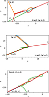 |
Fig. 4. Three examples of how the braid I.A.4i.c.(0.5) forms from an encounter between a binary (a,b) and two single stars (c and d), between two binaries (a,b and c,d), and a triple (a,b,c) encountering a single (d). |
4.3. Braid progenitors
In Fig. 5 we present the orbital separations of the two binaries for braid model A, the one with a fBB = 0.83 in Table 2 or 242 binary pairs. The inner and outer binaries have ⟨ain⟩≃0.30 with a median of  . For the outer orbit we find ⟨aout = ⟩ ≃ 52 with a median of
  . For the other braids, the media have a similar range. It turns out that braids tend to dissolve in a very tight and one very wide binary. The braids also tend to dissolve in a hierarchical triple (one with a tight inner a rather wide outer orbit).
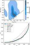 |
Fig. 5. Model A distributions of orbital elements, semimajor axes, and eccentricities for an interaction resulting in a binary–binary with fBB = 0.058 (see Table 2). Top: Semimajor axis of the two binaries. We present the tighter binary along the x-axis and the wider binary along the y-axis (explaining the empty lower-right corner bordered by the dashed line). Bottom: Eccentricity distributions of various orbits. The Kolmogorov-Smirnov test indicates that for model A, the tighter and wider distributions for eccentricity are indistinguishable. For the Figure-8 (p = 0.0064) and |

The eccentricity (e) distribution of the two binaries in which a braid separates is strongly peaked toward unity. Objects in our calculations were point masses, and collisions or gravitational wave radiation were ignored. But if we were to introduce (reasonable) finite radii, ≳10% of interactions would lead to collisions, rather than a stable pair of binaries. To guide the eye, and illustrate the skewness of the eccentricity distribution, we overplot curves for f(e)∝e2, ∝e3, and ∝e4, in Fig. 5. A distribution f(e)∝e2 would naively be consistent with expectations based on virialized few-body scattering (Heggie 1975). However, a steeper distribution toward high eccentricities is expected for encounters between hard pairs of particles (Ginat & Perets 2024). It raises the intriguing possibility that a braid could form from a four-body encounter in which two objects experience a collision, leaving the collision product and the other unaffected objects in a braid.
4.4. Braid formation cross section
In Fig. 6 we present the interaction result from launching particle m4(t = 0)≡min, with velocity vin, and impact parameter din into the braid from model A. We performed six series of calculations for each parameter, marginalizing over the direction (ϕ) from which the particle was injected. We performed similar calculations for the other braids, but the figures are insufficiently different to present. Except for the effect of vin for braid  , which we present in Fig. 7, showing quite different results. It is interesting to note that, together with the Figure-8, this braid is linearly stable.
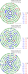 |
Fig. 6. Result of the encounter with model A when varying vin (top), m4 (middle), and din (bottom) for six values of the free parameter. The results are presented along the circle ϕ, and the parameter values corresponding to the concentric circles are indicated along the scale bar on the top middle to right of each figure. To the bottom right, we show the fraction of interactions that resulted in a binary–binary (blue) and a triple–single (red). These colors also correspond to the colors of the bullets in the concentric circles, and open green circles indicate the most common result of a binary with two singles. For comparison, the circle in the top panel is identical to the second (from the inside) circle in the middle panel. The second circle in the top panel is identical to the inner circle in the bottom panel. |
The circles with outcome statistics in Fig. 6 illustrates irregularity in the solution space. Although outcomes are dominated by binary and two single escapers (green circles), the binary-binary formation channel and triple-single channel are prevalent. For this model, when the incoming velocity v4 ≳ 4, encounters fail to result in two binaries.
On the other hand, even higher incoming velocities tend to lead to the survival of the braid, rather than to the formation of a hierarchical triple. In Fig. 6 we do not make the distinction between a surviving braid (democratic triple) and the more usual outcome in the form of a hierarchical triple; both are indicated by red dots in Fig. 6. This trend is even more pronounced in Fig. 7, where the braids in the outermost ring (highest incoming velocity) survives in 22.8% of the cases. When injected along the braid’s long axis, the encounter tends to lead to a binary and two singles, or four singles. In Fig. 7 we present the simulation results for braid  with v4 as the free parameter. One of the striking differences compared to Fig. 6 is the relatively large proportion of triples formed when the velocity of the incoming particle, |v4| ≳ 8.

However, when injected perpendicular to the braid’s long axis (around 45° ≲ϕ ≲ 135° and 225° ≲ϕ ≲ 315°) the encountering objects tend to fly through the braid without doing much damage. The other models (Figure-8, model A, and I.A.4i.c.(0.5)), being more symmetric, are less prone to such harmless penetrating encounters. It is interesting to note that the survivability of the braid (or the preservation of the democratic triple) as a result of a penetrating encounter seems not to depend on stability, or the Lyapunov timescale.
4.5. The third dimension
So far we have examined the planar problem, in which all participating particles are in the same plane. Since this is rather restricted, we also explored the possibility forming a planar braid given a nonplanar interaction. We realized this by injecting the incoming particle from a random direction into the planar braid. In this experiment the braid is orbiting in the X-Y Cartesian plane with zero azimuth (θ = 0). The incoming particle is injected isotropically from azimuth θ ∈ [ − 180° ,180° ] and polar angle ϕ ∈ [ − 90° ,90° ]. In Fig. 8 we present the Mollweide projection of one such cases for the Figure-8 problem for two incoming velocities: vin = 0, and vin = 2.
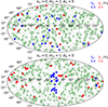 |
Fig. 8. Mollweide projection (azimuth along the x-axis and polar angle) for encounters of the Figure-8 braid with vin = 0 (top) and vin = 2 (bottom). The other parameters are m = 1 and d = 0. Each simulation was run 300 times with η = 0.01. For the legend of the symbols, see Fig. 6. |
The fraction of interactions that produce braids in the nonplanar case is statistically indistinguishable from that in the planar case, for binary-binary as well as for the triple-single encounters.
Certain areas in parameter space are preferred for specific interactions. This trend becomes even more pronounced for higher initial incoming velocities. For the Figure-8 solutions (adopting min = 1, and din = 0) braids, a low value of vin = 0 does not lead to an appreciable anisotropy in the initial conditions for forming braids either from binary-binary or triple-single encounters. However, as illustrated in Fig. 8, for vin = 2 binary-binary encounters are significantly more concentrated to low values of the azimuth and polar angles. This trend of clustering is comparably pronounced in the model A, and  braids, but is notoriously absent for I.A.4i.c.(0.5), which does not show this.
To test the anisotropic distribution of the various simulation results, we checked if the mean vector length is close to zero using the Rayleigh test for uniformity on the sphere. Under isotropy, the test statistic R2/N (where R is the resultant vector length and N is the number of points) should be ≲3 (for sufficiently large N). The results of this analysis are presented in Table 3.
Chi-squared values for the Rayleigh test.
4.6. The fractality of the initial phase-space
The distribution of the incoming angles suggest a fractal distribution in parameter space. For that reason we calculated the fractal (box counting) dimension (D) for each of the distributions (see Table 3). To quantify this statement, we present in Fig. 8 the fractal dimension by mapping the azimuth and polar angles on a two-dimensional grid, and subsequently apply box-counting to estimate the fractal dimension from how the number of occupied boxes scales with box size. The results are presented in Table 4.
Fractal dimension for the distributions.
All binary-single-single encounters correspond to a fractal dimension D ∼ 1: the resulting parameter space maps homogeneously on azimuth and polar angle. We saw this already in relation to Fig. 8 (green circles), and the Rayleigh test results in Table 3. The binary-binary and triple-single encounters, however (irrespective of the braid model or the incoming velocity, vin) are clustered or lie along a curve in azimuth and polar angles, rather than a uniform filling of the parameter space. Although the amount of data in our experiment is rather limited, we argue that these clusterings are related to the chaotic behavior of four-body encounter. A similar clustering and patched stability was observed in three-body encounters as islands of stability in a sea of chaos (Trani et al. 2024).
4.7. The effect of numerical accuracy
In our experiment we relied on the reversibility of Newton’s equations of motion. However, the numerical method adopted is not precisely time-reversible. We did not perform converged solution simulations because our analysis is strictly of a statistical nature. Small errors when integrating in one direction may indeed result in the reversible solution failing to lead to the same initial conditions. In principle, this would render the numerical result apprehensive (Portegies Zwart & Boekholt 2018).
The interactions, however, are generally short (lasting < 10 braid orbits), and the original braids have a long Lyapunov timescale (≳1000 orbits). As a consequence, the chaotic behavior of the systems hardly has time to cause numerical errors to grow substantially. The vast majority of interactions have a relative energy error < 10−5, which should suffice for a statistical scientific interpretation. In some cases, the energy error at the end of the simulation is larger, but these are not systematically associated with one of the interactions of interest. We therefore consider our results to be robust and not systematically affected by numerical effects.
To further support this, we performed an additional series of simulations based on the Figure-8 braid. In Fig. 9 we present the effect of numerical accuracy on the simulation results. Each circle shows the results (see the legend and explanation in Fig. 6) for a series of simulations for a specific value of the time-step parameter η, which we varied from 0.01 (inner most circle) to 0.1 (outer most circle). Not shown is a series of runs for η = 0.001, but the results are statistically indistinguishable from η = 0.01.
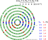 |
Fig. 9. Result of the encounter for the Figure-8 braid for vin = 1, min = 1, and din = 0 and for various values of the numerical time-step parameter (η). The η tunes the time-step of the numerical integration. The default choice in our simulations, η = 0.01 (represented by the inner most circle), is relaxed here for circles farther out, which represent less accurate integrations. Each set of runs contains 300 solutions for that particular value of η. |
The various fractions of simulation outcomes are presented to the right of the figure (as in Fig. 6). For this case, the canonical rate at which a braid forms from two binaries is about 2.6 with a comparable dispersion. Statistically, the probability of a braid forming through a binary-binary encounter or through a triple-single encounter are independent of integration accuracy.
5. Conclusion
We integrated four different three-body braids, perturbing them with a fourth particle and evolving until dissolution. Most braids separated into a binary plus two singles, ∼5% separated into two binaries, and ∼3% formed a triple with one escaper.
When the incoming velocity exceeds the braid’s binding energy, the braid may survive temporarily. Symmetric braids dissolve readily under such strong perturbations, while less symmetric ones may survive if encountered along the short axis. For instance, braid  withstands broadside impacts, whereas model A breaks into four singles or a binary and two singles.
Reversing ionizing encounters confirms that Figure-8 braids can form from encounters between two binaries (Heggie 2000). These binaries typically have high eccentricities, ⟨e⟩ = 0.80 ± 0.22, with a distribution skewness (Sk ∼ −1.26) to even higher eccentricities, exceeding those of typical Galactic (⟨e ⟩∼0.6) and Kuiper belt (⟨e ⟩∼0.2) binaries. This implies that favored initial binary parameters are uncommon.
Braid-formation cross sections for binary–binary (∼5%) to triple–single (∼3%) encounters partially offsets the rareness of suitable binaries. Near-coplanar orbital planes, however, are required, further restricting formation. Despite this, considering triples and diverse configurations, braids may be quite common in the Galaxy (Heggie 2000).
Although the majority of our calculations were performed in a plane, we relaxed this assumption by allowing nonplanar interactions. Although our parameter-space coverage for this generalized approach is limited to varying a few of the free parameters over a limited range, our findings show that braids can form a wide range of parameters, including nonplanar encounters.
We observe that the parameter-space distribution of forming braids is anisotropic and has a relatively low fractal dimension, forming distributions in azimuth and polar angles in a two-dimensional space (much like the earlier work of Jackson Pollock, rather than his late works). The anisotropy of the initial parameter space becomes more pronounced for higher incoming velocities.
Braids are more likely to survive in shallow gravitational potentials, for example trans-Neptunian objects, the Oort cloud, the Galactic halo, and intergalactic space. The high Kuiper belt binary fraction is evidence that transient braids exist in these regions (Noll et al. 2008).
Finite object sizes of astronomical objects suggest braids can form from collisions during binary–binary or binary–triple interactions. Stellar braids often lead to collisions unless objects are compact, suggesting black hole or neutron star braids might form and be detectable via gravitational waves. In addition, massive high-velocity runaway stars could form from ionized braids, as one (or both) of the binaries of the dissolved braid is prone to the two stars colliding.
Data availability
All runscripts and data generated for this paper are available on Zenodo under doi https://doi.org/10.5281/zenodo.18403805. The work was done with AMUSE, which can be downloaded from amusecode.org.
Acknowledgments
We thank Douglas Heggie, Anna Lisa Varri, and Tjarda Boekholt for discussing braids. We also thank the referee for the suggestion to include a discussion on the non-planarity of the problem. SPZ is deeply indebted to his friend Joost Visser for joining the expedition by ferry and train to Edinburgh and attending the Edinburgh Chaotic Rendez-vous in September 2025.
References
- Boekholt, T., & Portegies Zwart, S. 2015, Comput. Astrophys. Cosmol., 2, 2 [NASA ADS] [CrossRef] [Google Scholar]
- Chenciner, A., & Montgomery, R. 2000, Ann. Math., 152, 881 [CrossRef] [Google Scholar]
- Chenciner, A., Gerver, J., Montgomery, R., & Simó, C. 2002, in Simple Choreographic Motions of N Bodies: A Preliminary Study, eds. P. Newton, P. Holmes, & A. Weinstein (New York, NY: Springer), 287 [Google Scholar]
- Ginat, Y. B., & Perets, H. B. 2024, MNRAS, 531, 739 [Google Scholar]
- Heggie, D. C. 1975, MNRAS, 173, 729 [NASA ADS] [CrossRef] [Google Scholar]
- Heggie, D. C. 2000, MNRAS, 318, L61 [Google Scholar]
- Heggie, D. C., & Mathieu, R. D. 1986, in The Use of Supercomputers in Stellar Dynamics, eds. P. Hut, & S. L. W. McMillan (Berlin: Springer Verlag), Lect. Notes Phys., 267, 233 [NASA ADS] [CrossRef] [Google Scholar]
- Henon, M. 1976, Celest. Mech., 13, 267 [NASA ADS] [CrossRef] [Google Scholar]
- Homburg, A. J., & Knobloch, J. 2024, Bifurcation Theory (American Mathematical Society), 246 [Google Scholar]
- Kajihara, Y., Kin, E., & Shibayama, M. 2023, Topol. Appl., 337, 108640 [Google Scholar]
- Kapela, T., & Simó, C. 2007, Nonlinearity, 20, 1241 [Google Scholar]
- Kepler, J. 1609, Astronomia Nova, 1 [Google Scholar]
- Li, X., Jing, Y., & Liao, S. 2018, PASJ, 70, 64 [Google Scholar]
- Li, X., Li, X., & Liao, S. 2021, Sci. China Phys. Mech. Astron., 64, 219511 [Google Scholar]
- McMillan, S., Portegies Zwart, S., van Elteren, A., & Whitehead, A. 2012, in Advances in Computational Astrophysics: Methods, Tools, and Outcome, eds. R. Capuzzo-Dolcetta, M. Limongi, & A. Tornambè, ASP Conf. Ser., 453, 129 [Google Scholar]
- Montgomery, R. 1998, Nonlinearity, 11, 363 [NASA ADS] [CrossRef] [Google Scholar]
- Moore, C. 1993, Phys. Rev. Lett., 70, 3675 [NASA ADS] [CrossRef] [Google Scholar]
- Newton, I. 1687, Philosophiae Naturalis Principia Mathematica, 1 [Google Scholar]
- Noll, K. S., Grundy, W. M., Chiang, E. I., Margot, J.-L., & Kern, S. D. 2008, in Binaries in the Kuiper Belt, eds. M. A. Barucci, H. Boehnhardt, D. P. Cruikshank, A. Morbidelli, & R. Dotson, 345 [Google Scholar]
- Orwell, G. 1949, Nineteen Eighty-Four (London: Secker& Warburg), first edition published June 8, 1949 [Google Scholar]
- Poincaré, H. 1891, Bull. Astron. Ser. I, 8, 12 [Google Scholar]
- Portegies Zwart, S. F., & Boekholt, T. C. N. 2018, Commun. Nonlinear Sci. Numer. Simul., 61, 160 [NASA ADS] [CrossRef] [Google Scholar]
- Portegies Zwart, S., & McMillan, S. 2018, Astrophysical Recipes; The Art of AMUSE [Google Scholar]
- Portegies Zwart, S., McMillan, S., Harfst, S., et al. 2009, New Astron., 14, 369 [Google Scholar]
- Portegies Zwart, S. F., Boekholt, T. C. N., Por, E. H., Hamers, A. S., & McMillan, S. L. W. 2022, A&A, 659, A86 [NASA ADS] [CrossRef] [EDP Sciences] [Google Scholar]
- Schubart, J. 1956, Astron. Nachr., 283, 17 [Google Scholar]
- Simó, C. 1994, Publication Details or Conference Proceedings [Google Scholar]
- Simó, C. 2001, European Congress of Mathematics: Barcelona, July 10–14, 2000 (Springer), I, 101 [Google Scholar]
- Simó, C. 2002, Contemporary Mathematics, 292, 209 [Google Scholar]
- Terracini, S. 2022, in N-Body Problem and Choreographies, ed. G. Gaeta (New York, NY: Springer US), 357 [Google Scholar]
- Trani, A. A., Leigh, N. W. C., Boekholt, T. C. N., & Portegies Zwart, S. 2024, A&A, 689, A24 [NASA ADS] [CrossRef] [EDP Sciences] [Google Scholar]
We followed Orwell’s “Ignorance is strength” philosophy in this perspective (Orwell 1949, see p. 6).
All Tables
All Figures
|
Fig. 1. The four three-body braids adopted in this study: the classic Figure-8 problem (top) and three more complicated braids, the unequal-mass problem, I.A.4i.c.(0.5), and |
| In the text | |
|
Fig. 2. Two representations of braid I.A.4i.c.(0.5) after 100 time units. Top: Unperturbed solution integrated for ten N-body time units. Bottom: Result of the perturbed solution in the same time frame. The introduced perturbation was 10−5 in the x coordinate. Both solutions have clearly deviated from the original braid, and from each other. By this time, the phase space distance between the two solutions is on the order of unity. The orbits are unstable, and in the next 100 crossing times, one particle is ejected. |
| In the text | |
|
Fig. 3. Braid model A after 106 N-body time units. By this time, an initial perturbation of 10−5 has grown to O(10−2). The braid still resembles the original, but the entire orbit has been precessing. |
| In the text | |
|
Fig. 4. Three examples of how the braid I.A.4i.c.(0.5) forms from an encounter between a binary (a,b) and two single stars (c and d), between two binaries (a,b and c,d), and a triple (a,b,c) encountering a single (d). |
| In the text | |
|
Fig. 5. Model A distributions of orbital elements, semimajor axes, and eccentricities for an interaction resulting in a binary–binary with fBB = 0.058 (see Table 2). Top: Semimajor axis of the two binaries. We present the tighter binary along the x-axis and the wider binary along the y-axis (explaining the empty lower-right corner bordered by the dashed line). Bottom: Eccentricity distributions of various orbits. The Kolmogorov-Smirnov test indicates that for model A, the tighter and wider distributions for eccentricity are indistinguishable. For the Figure-8 (p = 0.0064) and |
| In the text | |
|
Fig. 6. Result of the encounter with model A when varying vin (top), m4 (middle), and din (bottom) for six values of the free parameter. The results are presented along the circle ϕ, and the parameter values corresponding to the concentric circles are indicated along the scale bar on the top middle to right of each figure. To the bottom right, we show the fraction of interactions that resulted in a binary–binary (blue) and a triple–single (red). These colors also correspond to the colors of the bullets in the concentric circles, and open green circles indicate the most common result of a binary with two singles. For comparison, the circle in the top panel is identical to the second (from the inside) circle in the middle panel. The second circle in the top panel is identical to the inner circle in the bottom panel. |
| In the text | |
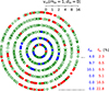 |
Fig. 7. Same as Fig. 6 but for braid |
| In the text | |
|
Fig. 8. Mollweide projection (azimuth along the x-axis and polar angle) for encounters of the Figure-8 braid with vin = 0 (top) and vin = 2 (bottom). The other parameters are m = 1 and d = 0. Each simulation was run 300 times with η = 0.01. For the legend of the symbols, see Fig. 6. |
| In the text | |
|
Fig. 9. Result of the encounter for the Figure-8 braid for vin = 1, min = 1, and din = 0 and for various values of the numerical time-step parameter (η). The η tunes the time-step of the numerical integration. The default choice in our simulations, η = 0.01 (represented by the inner most circle), is relaxed here for circles farther out, which represent less accurate integrations. Each set of runs contains 300 solutions for that particular value of η. |
| In the text | |
Current usage metrics show cumulative count of Article Views (full-text article views including HTML views, PDF and ePub downloads, according to the available data) and Abstracts Views on Vision4Press platform.
Data correspond to usage on the plateform after 2015. The current usage metrics is available 48-96 hours after online publication and is updated daily on week days.
Initial download of the metrics may take a while.