| Issue |
A&A
Volume 707, March 2026
|
|
|---|---|---|
| Article Number | A353 | |
| Number of page(s) | 10 | |
| Section | Stellar structure and evolution | |
| DOI | https://doi.org/10.1051/0004-6361/202558384 | |
| Published online | 18 March 2026 | |
A mapping method of age estimation for binary stars: Application to the α Centauri system A and B
1
Université Côte d’Azur, Observatoire de la Côte d’Azur, CNRS, Laboratoire Lagrange, France
2
Lomonosov Moscow State University, Sternberg Astronomical Institute, Moscow, Russia
★ Corresponding author: This email address is being protected from spambots. You need JavaScript enabled to view it.
Received:
3
December
2025
Accepted:
20
January
2026
Abstract
Context. Binary and multiple star systems are abundant, and they are important for determining the ages of exoplanet systems and Galactic populations. Given the wealth of data provided by Gaia and the upcoming PLATO mission, it is essential to improve stellar models to obtain accurate stellar ages. Multiple systems reduce the degeneracy in the stellar parameters that control evolution, and they allow better constraints on the physical processes at work in stellar interiors.
Aims. Our objective is to apply a mapping technique to estimate the age of a system and the initial chemical composition. We also evaluate the influence of observational uncertainties in mass and heavy-element mixtures on results.
Methods. We applied an inverse calibration method to the evolution of a multiple stellar system, assuming that the stars share the same age and initial chemical composition. This approach determines age, the initial mass fractions of helium (Yini) and heavy elements (Zini), as well as the convective mixing-length parameters (αA and αB). It uses the observed luminosities (LA and LB), radii (RA and RB), and surface chemical compositions (Z/XA and Z/XB).
Results. We used the most recent observational data for M, R, L, and [Fe/H] of α Centauri A and B as input data for our method. We compared two assumptions for the Z/X ratio, following the results for the solar composition. For an assumed high solar Z/X⊙ = 0.0245, we obtain an age of 7.8 ± 0.6 Ga, Yini = 0.284 ± 0.004, and Zini = 0.0335 ± 0.0015. For a low solar Z/X⊙ = 0.0181, the derived age is 8.7 ± 0.6 Ga, Yini = 0.267 ± 0.008, and Zini = 0.025 ± 0.002. Observational errors in the stellar masses of ±0.002 lead to an age error of 0.6 Ga. Overshooting of 0.05 − 0.20Hp at the boundary of the convective core increases the age by 0.6 − 2.1 Ga. Models with higher Z/X and radiative cores, with ages of 7.2 − 7.8 Ga, appear preferable and show better agreement with the observed asteroseismic frequencies.
Key words: binaries: general / stars: evolution / stars: fundamental parameters / stars: individual: alpha Centauri A / stars: individual: alpha Centauri B
© The Authors 2026
 Open Access article, published by EDP Sciences, under the terms of the Creative Commons Attribution License (https://creativecommons.org/licenses/by/4.0), which permits unrestricted use, distribution, and reproduction in any medium, provided the original work is properly cited.
This article is published in open access under the Subscribe to Open model. This email address is being protected from spambots. You need JavaScript enabled to view it. to support open access publication.
1. Introduction
Studies of stars in binary systems have been carried out for decades using a variety of methods and observational data with differing levels of precision and constraint. Compared to single stars, binaries offer notable advantages, most importantly the ability to impose tighter constraints on stellar ages and to test the uniqueness of calibrated stellar models.
A well-known example is the multiple system α Centauri (Morel et al. 2000), one of the first binaries to be calibrated with a modern approach. The α Centauri system consists of α Centauri A and B, two Sun-like stars in a close binary orbit, and α Centauri C (Proxima Centauri), a low-mass red dwarf. Their proximity and solar-like nature make α Centauri A and B benchmark stars for calibrating stellar evolution models. The binary configuration enables robust determination of age and composition, making the system ideal for testing age-dating tools used in future studies of Galactic populations.
Another binary star, ζ Herculis, was calibrated before α Centauri (Chmielewski et al. 1995). The authors applied evolutionary tracks simultaneously to both components and predicted asteroseismic frequencies for comparison with observations. They concluded that the system remained insufficiently constrained, particularly in stellar masses and parallax. A subsequent recalibration aimed to improve upon this earlier analysis (Morel et al. 2001).
With the advent of high-precision parallaxes from the Gaia mission, particularly for numerous binary systems with accurately measured masses and for multiple systems in clusters, it is now timely to revisit such targets to test and refine calibration methods. Expanding the analysis to both binaries and higher-order multiples will enable more precise stellar age determinations, thereby improving the accuracy of age tagging for stellar populations across the Milky Way.
This work considers the development of a numerical method for calibrating multiple systems. We used recent high-precision measurements of stellar masses, luminosities, and radii, which are essential inputs for binary modeling. Our goal was to create an automated tool to determine the age and initial chemical composition, specifically the initial helium mass fraction (Yini) and heavy-element mass fraction (Zini), of binary star systems. The method uses observational constraints such as stellar masses, radii, luminosities, and surface metallicity ratios (Z/X). A central assumption is that both stars formed simultaneously and therefore share the same age and initial composition.
We aimed to address key questions: Does a physically consistent solution exist for the given constraints? If so, is the solution unique? How do observational uncertainties and the assumed heavy-element mixture influence the results?
For broad applicability, we did not include seismic constraints in our general calibration, as asteroseismic frequency data for binaries remain scarce, despite their demonstrated ability to significantly improve age estimates (Joyce & Chaboyer 2018). However, for the test on α Centauri, we used available seismic data to assess our solution, while noting that the number of detected frequencies is still limited.
In Sect. 2, we develop the inversion mapping method. We test our tool on the α Centauri system in Sect. 3. Our conclusions are summarized in Sect. 4.
2. The inverse mapping method for stellar calibration
2.1. Mathematical formulation of the problem
We present a mathematical formulation of the problem of modeling stars A and B in a binary system. The key concept is a stellar evolutionary track as a mapping from one space to another. The evolutionary track is defined as a sequence of models for a star with mass Mj, which maps the three initial parameters of the star {αj, Yini, and Zini} to the three observed parameters {R, L, and Z/X}j at each assumed stellar age ts. Here, the index j refers to star A or B. We define Yini as the initial helium mass fraction, Zini as the initial heavy-element mass fraction (i.e., elements heavier than helium), αj as the mixing-length parameter, R as the stellar radius, L as the luminosity, and Z/X as the ratio of heavy-element to hydrogen mass fractions.
The idea of evolutionary mapping originates from Noels et al. (1991). An extensive review of its applications is provided by Guenther & Demarque (2000). Mathematically, direct evolutionary mapping is expressed as
![Mathematical equation: $$ \begin{aligned} E(M_j): \left[ \{\alpha _j,Y_{\mathrm{ini} },Z_{\mathrm{ini} }\} \xrightarrow {t_s} \{R,L,Z/X\}_j \right], \end{aligned} $$](/articles/aa/full_html/2026/03/aa58384-25/aa58384-25-eq1.gif) (1)
(1)
where ts is the stellar age and serves as a parameter of the mapping. This formulation represents a set of evolutionary tracks as functions of age, specific to each stellar component. We analyze the mapping by examining these evolutionary tracks across the relevant parameter space.
Our goal is to identify, among all possible tracks, a pair of evolutionary tracks EA(t) and EB(t) that correspond to the given observed parameters  of stars A and B. The resulting tracks must satisfy the binary constraints: they must have the same age (tA = tB), and also have the same initial chemical composition {Yini, Zini}A = {Yini, Zini}B. To solve the problem, we introduce an inverse mapping E−1:
![Mathematical equation: $$ \begin{aligned} E^{-1}(M_j): \left[ \{R,L,Z/X\}_j^{\mathrm{observed} } \xrightarrow {t_s} \{\alpha _j,Y_{\mathrm{ini} },Z_{\mathrm{ini} }\} \right]. \end{aligned} $$](/articles/aa/full_html/2026/03/aa58384-25/aa58384-25-eq3.gif) (2)
(2)
In Eq. (2), we do not require equality of the convection parameters αA and αB. The values of αA and αB can differ. We do not impose prior assumptions on these parameters.
When considering a single star, we have three known parameters (R, L, and Z/X) and three unknown (αj, Yini, and Zini); the problem is determined for every fixed time ts. For a pair of stars, there are six known parameters (RA, LA, (Z/X)A, RB, LB, and (Z/X)B) and five unknowns (ts, Yini, Zini, αA, and αB). The problem is overdetermined. The observed parameters  naturally include measurement uncertainties. Assessing the impact of these observational errors is fundamental; we address this in our analysis of α Cen. However, when defining the stellar evolutionary tracks and formulating the binary system constraints, we do not include these errors.
2.2. Inverse mapping method
Computing an inverse mapping in explicit form is challenging. We used sequential iterations and inverted the differential of the evolutionary map Eq. (1).
For a single star, the mapping provides a one-to-one correspondence between two 3D parameter spaces. It is differentiable with respect to the three input parameters Pini = {αj, Yini, Zini}. Therefore, we constructed the differential of the mapping via the Jacobian matrix, which captures the sensitivity of the observable parameters to variations in the initial stellar parameters,
 (3)
(3)
The Jacobian JE is a matrix 3 × 3 that depends on the assumed age of the system. It must be non-singular, i.e., its determinant must be nonzero, det(JE)≠0. If this condition is not fulfilled, the inverse mapping has no solutions or infinitely many solutions.
The properties of the Jacobian are straightforward. It allows us to determine how much the observed (target) parameters T = {R, L, Z/X} of the star change in response to a variation in the initial parameters by a vector δPini, such that
 (4)
(4)
The dot in Eq. (4) denotes matrix multiplication.
The core principle of our method is that the search for the inverse mapping E−1 is replaced by the calculation of the inverse Jacobian JE−1. This inverse matrix enables an efficient determination of the initial stellar parameters that produce the observed parameters T. The process is iterative. If the difference between the observed parameters of the currently constructed evolutionary track, E(i)(ts), and the target point, T, is ΔiT = T − E(i)(ts), we use as the next approximation for the track i + 1:
 (5)
(5)
The convergence of the iterative process is generally rapid: typically, around 12 iterations are sufficient for star A, and only about five iterations are needed for star B.
The inverse Jacobian method facilitates the study of the influence of observational errors on the evolutionary track. It is sufficient to estimate the perturbations of the observational quantities ΔTobs and use Eq. (5), to determine the effect of observation errors on the track parameters. The inverse Jacobian JE−1 depends weakly on the desired track parameters. We computed JE for a sequence of ages, but used only the closest in age for the calculations.
Calculations of suitable parameters  were carried out for the entire series of ages ts. As a result, we obtained a sequence of initial parameters {α(ts),Yini(ts),Zini(ts)} under which the mapping E should fall within the given values of the observed parameters T. If necessary, the approximations for
  can be refined by applying Eq. (5) and calculating the corresponding tracks.
The inverse calibration method is most suitable for solar-type stars on the main sequence. For older stars, applying the method appears problematic. For late spectral type stars with masses below 0.8 M⊙, further study is required. Estimating critical uncertainty levels for mass, radius, and luminosity, which render the method ineffective, is generally difficult and requires case-by-case verification. Possible candidates for applying the method include α Centauri, 16 Cygni, and similar stars.
3. Application to α Centauri A and B
3.1. Input data
As mentioned previously, the nearby α Centauri system is a well-studied triple system, comprising the close binary α Centauri A and B, which are two Sun-like stars, and α Centauri C (Proxima Centauri), a low-mass red dwarf. Their proximity to the Sun and solar-like properties make α Centauri A and B benchmark stars for calibrating stellar evolution models. Their binary configuration enables more robust determination of age and initial composition (we account for the diffusion of elements over time in the computation of evolutionary tracks), making them ideal for testing tools used to estimate stellar ages in different Galactic populations. Table 1 provides a summary of representative observational data. For example, Kervella et al. (2017) derived precise values using the VLTI/PIONIER1 optical interferometer, which are used in modeling studies by Joyce & Chaboyer (2018) and Manchon et al. (2024). In contrast, Akeson et al. (2021), using the Atacama Large Millimeter/submillimeter Array (ALMA) as part of a planet-detection program via differential astrometry, report notably lower values for stellar mass, radius, and luminosity than those of Kervella et al. (2017). These discrepancies highlight the importance of cross-validating observational datasets when constructing accurate models of stellar evolution. We tested our model using these binary stars.
Results from recent observations of α Centauri A and B.
For our analysis, we used data from Akeson et al. (2021) and Morel (2018) (Table 1). We assumed that the stellar masses were known. We adopted MA = 1.0788M⊙ and MB = 0.9092M⊙. We analyze the impact of mass uncertainties in Sect. 3.4.1 and 3.4.3. The observations provide the metallicity [Fe/H], from which the ratio Z/X is derived:
![Mathematical equation: $$ \begin{aligned} \left(\frac{Z}{X}\right)_* = \left(\frac{Z}{X}\right)_\odot \cdot 10^{[\mathrm{Fe} /\mathrm{H} ]^{*}_{{\odot }}}. \end{aligned} $$](/articles/aa/full_html/2026/03/aa58384-25/aa58384-25-eq11.gif) (6)
(6)
We computed (Z/X)* using a solar ratio (Z/X)⊙ = 0.0245 from Grevesse & Noels (1993), which corresponds to a high-Z mixture. This solar (Z/X)⊙ remains a subject of debate (see, for example, the review of Christensen-Dalsgaard 2021). Acceptance of a low-Z solar mixture (Z/X)⊙ = 0.0181 (Asplund et al. 2009) would alter the calibration results, although the observed [Fe/H] remains fixed. We discuss this sensitivity in Sect. 3.4.2.
3.2. The CESAM2k stellar evolution code
We performed all computations using the 1D stellar evolution code CESAM2k (Morel & Lebreton 2008; Manchon et al. 2025). We treated convection using the mixing-length theory (Böhm-Vitense 1958). We calculated microscopic diffusion with coefficients based on Burgers equations (Burgers 1969), accounting for radiative acceleration. We used the OPAL 2005 equation of state (Rogers & Nayfonov 2002) and used the OPAL package for opacity calculations (Iglesias & Rogers 1991). Thermonuclear reaction rates follow the NACRE compilation (Angulo et al. 1999). We modeled the atmosphere using the fully radiative Eddington law (Eddington 1930). We initialized the evolutionary models at the pre-main sequence stage and assumed constant stellar masses throughout the evolution.
3.3. Stellar modeling results
First, we computed evolutionary tracks with masses MA and MB for sets of initial conditions (αMLT ± Δα, Yini ± ΔY, Zini ± ΔZ) to obtain the Jacobian Eq. (3). Second, we performed the inverse mapping using Eq. (5). Figure 1 shows the results of the inverse mapping. It presents the initial compositions of stars A and B that allow them to reach the observed parameters (R, L, Z/X)obs at a given age, with the ages indicated in the legend.
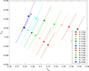 |
Fig. 1. Inverse mapping results. Initial conditions for stars A (circles) and B (stars) reproduce the observed parameters (R, L, Z/X)obs at given ages. Colors indicate the ages, as shown in the legend. Colored lines show the initial chemical compositions obtained by accounting for observation errors ±Δ(Z/X). The black line shows the common initial conditions (Yini, Zini) for which the stars achieve the observed values (R, L, Z/X ± Δ(Z/X))obs at ages from 7.801 to 7.826 Ga. |
The data for stars A and B trace two distinct curves in the (Yini, Zini) plane. To match the observable parameters at an earlier age (e.g., 2 Ga), a higher initial helium abundance, Yini, and a lower initial metallicity, Zini, are required compared to later ages (e.g., 8 Ga). Figure 1 shows that stars A and B share no common initial conditions (Yini, Zini) for any system age.
Fig. 1 also illustrates how observational uncertainties affect the inferred values of Yini and Zini. The impact of uncertainties in luminosity and radius is not visible at the scale of the figure. Uncertainties of ±Δ(Z/X) result in segments rather than single points, reflecting the range of possible initial conditions. For young stars A and B, the segments corresponding to the same age (i.e., the same color) are well separated. For example, the two brown segments, corresponding to a stellar age of 2 Ga, are separated by ΔYini ≈ 0.04. The two red segments, which correspond to an age of 3 Ga, are separated by ΔYini ≈ 0.03. Separation decreases with age; for example, the cyan segments corresponding to 7 Ga are separated by ΔYini ≈ 0.005. At a fixed Zini, star B has a larger Yini than star A. The blue segments (8 Ga) are very close to each other, with star B having a larger Yini than star A at fixed Zini. Therefore, points of common initial conditions between stars A and B begin to appear at ages between 7 and 8 Ga.
We next examine the (Yini, Zini) range within the 7 − 8 Ga interval to identify the initial conditions under which both stars simultaneously match the observed values (R, L, Z/X ± Δ(Z/X))obs at the same age. First, we fixed Zini, and for a given initial Yini, we selected αMLT such that the model falls within the observed ranges of luminosity and radius. This condition is satisfied at a specific stellar age. As illustrative cases, we chose Zini = 0.0320, which lies near the lower limit for star A, and Zini = 0.0350, near the upper limit for star B.
Figure 2 shows the stellar ages as a function of Yini for two metallicities, Zini = 0.0320 (solid lines) and 0.0350 (dashed lines). For Zini = 0.0320 and Yini = 0.2750, star A reaches its observed radius and luminosity at the age of 8.266 Ga, and star B at 8.605 Ga. As Yini increases, the stellar ages decrease.
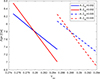 |
Fig. 2. Stellar ages as a function of Yini for Zini = 0.032 (solid lines) and 0.035 (dashed lines). |
The slopes of the Age(Yini) curves differ between stars A and B, leading to an intersection point where both stars reach their observed properties at the same age. For Yini = 0.2796, this common age is 7.826 Ga, representing a consistent solution for both stars. For Zini = 0.0350, the corresponding age at the intersection point is 7.801 Ga.
The two identified solutions appear as black asterisks in Fig. 1. Other possible pairs lie between these two limits (black segment in Fig. 1) and slightly beyond them. Table 2 summarizes the corresponding initial conditions, mixing-length parameters, and stellar ages for these models. Figure 3 presents an example of the evolutionary tracks for Zini = 0.032.
Calibration results: Initial compositions, mixing-length parameters, and ages for stars A and B.
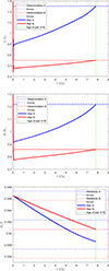 |
Fig. 3. Examples of evolutionary tracks of stars A and B for luminosity (upper panel), radius (middle panel), and Z/X (lower panel), all with Zini = 0.0320. The age of the pair is 7.826 Ga, corresponding to the intersection point in Fig. 2. |
In the bottom panel, the evolution of Z/X for star A does not reach the observed metallicity Z/X = 0.0423 at 7.826 Ga. This occurs because no exact solution reproduces both stars within the exact Z/X values given in (Morel 2018). However, our problem formulation seeks to find a solution that satisfies modern observations within the error limits ±ΔZ/X. Our solution satisfies this condition.
Notably, the metal-to-hydrogen mass fraction Z/X decreases more rapidly during the evolution of star A than during that of star B. The rate of settling of heavy elements from the convective zone in solar-like stars depends on the relative mass of the convective zone,  . The larger the mass of the convective zone, the smaller the relative fraction of precipitated metals. For star A, the relative mass of the convective zone is 0.035, and for star B it is 0.066. This explains the difference in settling rates shown in Fig. 3. However, observations indicate that star A has a higher present-day Z/X than star B. We can reconcile this apparent contradiction only by considering the uncertainties in the observational data.
Both stars, A and B, have developed convective envelopes. In our method, the mixing-length parameter, α, has an evolutionary calibration meaning. In this context, it determines the stellar radius: varying α changes the stellar radius. This relationship arises from our Jacobian analysis, where the derivative ∂R/∂α is significantly greater than ∂L/∂α. Although our method determines α, we do not assign a strong physical meaning to the resulting values. We present different possible relationships between αA and αB.
3.4. Sensitivity of the solution to observational uncertainties
3.4.1. Impact of luminosity, radius, and mass uncertainties
The measured and estimated values of Z/X, luminosity, radius, and masses have associated uncertainties. In the previous section, we estimated how the uncertainty in Z/X affects the derived solution. Specifically, the uncertainties of Δ(Z/X) = ± 0.0050 result in an estimated stellar age uncertainty of ΔAge = ±0.0125 Ga.
We now assess the impact of other observational uncertainties (Table 1) on the derived stellar parameters. We adopt the solution for Zini = 0.0320 (model 1, Table 2) as the base model for the subsequent analysis. The results are presented in Table 3 and Appendix A. The first four rows show the results when luminosities vary by ΔLA/L⊙ = ±0.0019 and ΔLB/L⊙ = ±0.0007, resulting in an estimated age uncertainty ΔAge = ±0.0485 Ga. The next four rows present the results for uncertainties in the stellar radii, ΔRA/R⊙ = ±0.0055 and ΔRB/R⊙ = ±0.0036. These variations produce an age uncertainty ΔAge = ±0.1149 Ga. Finally, the mass uncertainties, ΔMA/M⊙ = ±0.0020 and ΔMB/M⊙ = ±0.0020, result in significantly larger age errors of ΔAge = ±0.6202 Ga (see the last four rows). Thus, we conclude that our age estimate is most sensitive to uncertainties in stellar masses.
Influence of observational errors on obtained results.
The most significant effect occurs when an input parameter is varied in opposite directions for stars A and B; for example, increasing the mass of star A while decreasing the mass of star B and vice versa. This indicates that the results are also sensitive to differences between the input parameters of stars A and B.
3.4.2. Impact of the solar mixture assumption
Morel (2018) report abundances in α Centauri relative to the solar value. However, the solar metallicity itself is subject to some uncertainty (e.g., Christensen-Dalsgaard 2021). In this section, we examine how the solar mixture assumption (low-Z versus high-Z) affects our results.
In addition to the total heavy-element mass fraction Z, the relative mass fractions of the individual elements differ between low-Z and high-Z mixtures. For example, oxygen is one of the most abundant heavy elements. Its logarithmic abundance is lgA(O) = 8.87 in the high-Z mixture (Grevesse & Noels 1993) and lgA(O) = 8.69 in the low-Z mixture (Asplund et al. 2009). The abundance of iron remains constant in both cases, lgA(Fe) = 7.50, but the relative mass fractions of other individual elements differ. These differences affect the plasma opacity, modify stellar models, and impact age estimates. For example, Guillaume et al. (2024) studied this effect in the Methuselah star (HD140283).
We performed computations for (Z/X)A = 0.0312 ± 0.005 and (Z/X)B = 0.0300 ± 0.005, based on the solar ratio (Z/X)⊙ = 0.0181 adopted from the low-Z mixture (Asplund et al. 2009). We used the corresponding opacity tables for this mixture of elements in the calculations. We find that the estimated age increases to 8.8 Ga. The initial helium abundance decreases to Yini = 0.259–0.276. The initial mass fraction of heavy elements also decreases to Zini = 0.023–0.027. The mixing-length parameters increase slightly, ranging from 2.2 to 2.3, but the difference between the two components remains below 0.03 (see Table 4, models 15 and 16).
Calibration results obtained for various input data.
3.4.3. Effect of alternative input parameters on the calibration
We examined the calibration results using the input parameters of (Kervella et al. 2017) and (Porto de Mello et al. 2008) in place of those of (Akeson et al. 2021) and (Morel 2018). Kervella et al. (2017) report higher masses, radii, and luminosities than Akeson et al. (2021), whose values we adopted in Sect. 3.3. In particular, the mass differences are ΔMA = 0.0267 M⊙ for star A and ΔMB = 0.0281 M⊙ for star B. These discrepancies arise from different observational methods.
As shown in Sect. 3.4.1, age estimates are highly sensitive to stellar masses, particularly to the mass difference between MA and MB. Other input parameters also affect the results. We examined a more complex scenario in which all input parameters vary simultaneously. We performed computations using the full set of input data – masses, radii, and luminosities – from (Kervella et al. 2017), along with the Z/X ratio from (Porto de Mello et al. 2008). In this case, we assumed that the metallicities of both stars are equal within uncertainties. For the high-Z solar mixture, we adopted the metallicity from (Grevesse & Noels 1993). We present the results in Table 4, model 17. The estimated age in this case is 9.2 Ga, which is 1.4 Ga older than the age derived using the input parameters from (Akeson et al. 2021). Therefore, adopting the parameters of (Akeson et al. 2021) yields a younger age estimate for α Centauri.
3.5. Acoustic properties of the stellar models
In this section, we examine the acoustic properties of the models for star A (see Tables 2–4). These models differ in age, in the presence or absence of a convective core, and in mass, luminosity, and radius – parameters that were varied within the limits of observational uncertainties.
For star B, only a few frequencies have been detected, which is insufficient for a detailed study comparable to that presented here for star A. We provide a brief discussion of star B at the end of this section.
3.5.1. Sound speed profiles in the stellar models
Figure 4 shows the sound speed profiles for the different models. In the convective zone, the profiles overlap, but in the radiative zone, between r/R* = 0.2 and 0.7, the sound speed in younger stars is lower than in older ones.
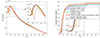 |
Fig. 4. Squared sound speed profile (left) and hydrogen mass fraction (right) for models of α Centauri A. |
In the central regions, at r/R* < 0.2, the situation is more complex. Models divide into two clear groups: those with a radiative core and those with a convective core.
In models with a convective core, the sound speed initially decreases with distance from the center, then rises sharply at the core boundary, and finally decreases smoothly. Models A15, A18, and A19 (Table 4) belong to this group and were computed using the low-Z solar mixture. Model A15 has an age of 8.8, while model A18, which includes overshooting at 0.05Hp, is slightly older, 9.4 Ga. Model A19 has an age of 10.9 Ga. The sound speed in the center of these models is noticeably higher than in those with a radiative core. Models that include overshooting are extensively discussed in Bazot et al. (2016).
Convective-core models retain hydrogen in their central regions, while radiative-core models have completely depleted it (Fig. 4). The presence of a convective core in star A remains an open question. Supporting radiative cores, de Meulenaer et al. (2010) found that models with radiative cores better reproduce the observed r10 and d13(n) frequency separations than those with convective cores. Similarly, Bazot et al. (2016) found that 60% of their models have radiative cores and 40% have convective cores. Nsamba et al. (2018, 2019) reported that 30% of their models have radiative cores, while 70% contain convective cores.
3.5.2. Asteroseismic frequencies to test the solution
Seismic frequencies were calculated on the basis of inverse-mapping stellar models using the ADIPLS (Christensen-Dalsgaard 2008) and GYRE (Townsend & Teitler 2013) oscillation codes. The discrepancies between these two calculation methods do not exceed 0.13 μHz, which is less than 0.1% of the absolute frequency values.
Roxburgh & Vorontsov (2003) showed that the large and small separation ratios were more convenient to analyze the stellar internal structure than the frequencies themselves, as these ratios are less sensitive to the outer layers. We consider the ratio r02,
 (7)
(7)
where small separation is
 (8)
(8)
and the large separation is
 (9)
(9)
Fig. 5 presents the results.
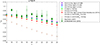 |
Fig. 5. Ratio r02(n) of small and large separations as function of radial order n for different models of α Centauri A (circles). Colors indicate the stellar age and diamonds show observational data. |
We verified whether our models are consistent with the frequencies published by Bazot et al. (2007) and de Meulenaer et al. (2010). We calculated r02 from these frequencies, using the mean when two values were available for a given combination of n and l. Figure 5 shows that our models, normalized to high-Z solar abundance, with radiative cores and ages 7.2–7.8 Ga lie along the lower edge of the observed ranges. Among them, the younger model A14 (7.2 Ga) provides the closest match.
The older the star, the lower its r02. This trend is slightly modified when the stellar masses vary. The mass effect depends on the mass ratio of stars A and B, which influences both the age calibration and, consequently, the frequencies. For example, the violet points represent model A14, in which we increased the mass of star A by 0.2% while simultaneously decreasing the mass of star B by 0.2% (see Table 3). This change reduces the calibration age to 7.2 Ga instead of 7.8 Ga (green points, model A1), producing a slight increase in the r02 ratio. Another example uses the stellar masses reported by Kervella et al. (2017) where the age of the pair is estimated to be 9.2 Ga, leading to a significant reduction in the r02 ratio (red points).
Adding overshooting to the A component with convective core increases the model ages in our solution. We obtain 8.79 Ga without overshooting, 9.43 Ga with overshooting of 0.05Hp, and 10.9 Ga with 0.20Hp. The increasing age of the solution is the dominant effect of overshooting. Consequently, the older model at 10.9 Ga exhibits a markedly lower r02 than the others (Fig. 5).
Salmon et al. (2021) studied the effect of overshooting, but on models of completely different ages. They found that the A component with overshooting of 0.20Hp has an age of 6.64 Ga, which differs significantly from our model. Therefore, we cannot directly compare the models with respect to r02.
Models A15 (orange points) and A17 (red points) have similar r02 despite different ages. This results from the interplay of several input parameters, particularly the abundances and masses. Radius and luminosity changes within observational uncertainties minimally affect the frequencies (blue and cyan points).
A similar discussion of the r02 ratio for star B is not possible due to the limited detected frequencies (Kjeldsen et al. 2005). Instead, we adopted a more traditional approach, comparing the observed and computed small frequency separations (Fig. 6). This analysis shows general agreement for all models of star B.
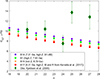 |
Fig. 6. Small separation d02 versus radial order n for α Centauri B. Models are shown as circles, and observational data by Kjeldsen et al. (2005) are shown as diamonds. |
3.6. Comparison with previous studies
Stellar masses are fundamental to analyses using evolutionary tracks. The adopted values for α Centauri A and B have evolved since the earliest studies. Over the past two decades, the estimated masses have changed by approximately 3%, reflecting advances in observational techniques and modeling precision. Consequently, researchers must interpret comparisons between studies with caution.
Researchers have estimated the age of α Centauri A and B multiple times using different methods (see Fig. 7). For example, Angus et al. (2015) used the gyrochronology approach and estimated the age of star A ( Ga) and star B (
 Ga) from their rotation periods. Morel (2018) performed a detailed abundance analysis of the spectra, deriving ages from indicators such as [Y/Mg] and [Y/Al] ( Y denotes yttrium). The ages inferred by Morel (2018) vary, ranging from 6.3 ± 1.3 Ga for certain abundance indicators, while others yield ages exceeding 8 Ga.
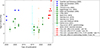 |
Fig. 7. Age of α Centauri A and B estimated in various works. The colors of the points indicate the method: blue, classic method without seismic data; green, seismic analysis; cyan, gyrochronology; orange, chemical analysis; and red, results of this study. |
The classic method to estimate the age of binary stars is evolutionary calibration without seismic data (blue points in Fig. 7). Guenther & Demarque (2000) provided one of the most comprehensive studies of α Centauri using this approach. They estimated the age as 7.6 Ga if star A has a convective core, or 6.8 Ga if it does not. Miglio & Montalbán (2005), Yildiz (2007) estimated the age as 8.9 Ga when seismic data were not included. Our method yields 7.2–10.9 Ga (red points in Fig. 7).
Incorporating seismic constraints into the calibration yields younger ages (green points in Fig. 7). Thévenin et al. (2002) first used asteroseismic frequencies to calibrate models, obtaining an age of 4.85 ± 0.5 Ga. Similarly, when researchers accounted for seismic data, several studies reported more tightly constrained age estimates, although they used older mass values: Eggenberger et al. (2004) found 6.52 ± 0.3 Ga, Miglio & Montalbán (2005) reported a range of 5.2–7.1 Ga, and Yildiz (2007) estimated 5.6–5.9 Ga. Using recent masses, Joyce & Chaboyer (2018) suggest an age of 5.3 ± 0.3 Ga and Salmon et al. (2021) report an age of 5.9–7.3 Ga.
Our results differ from Joyce & Chaboyer (2018) mainly due to assumptions about the different ages and initial chemical compositions of stars A and B. In Table 4 of Joyce & Chaboyer (2018), they allow differences in the initial chemical composition, with ΔYini ≤ 0.02, ΔZini ≤ 0.002, and in age, ΔAge = 0.02 Ga. Our approach differs: we seek solutions in which both stars share an identical chemical composition and age. However, if we allow such differences in the initial composition, our method cannot exclude 5.5–6.0 Ga as a possible solution (see Fig. 1).
Moreover, we excluded seismic constraints from our evolutionary calibration to maintain a general approach applicable to any stellar binary system, since asteroseismic frequency data for binaries remain relatively scarce despite their potential to significantly decrease age estimates. Instead, we used the available seismic frequencies solely to evaluate and validate our results within an asteroseismic context.
4. Conclusions
We developed and tested a method to map evolutionary tracks and estimate the age and initial chemical composition of stars in multiple systems, such as binaries, assuming a common evolutionary timescale. The method is based on the inversion of evolutionary tracks constrained by observational data.
We applied our method to the nearby and well-studied system α Centauri system to assess how uncertainties in the mass, radius, and luminosity of the two components affect the derived system age. Our age estimates span 7.2 and 10.9 Ga. Using the latest data (Akeson et al. 2021) yields an age of 7.8 Ga, which is 1.4 Ga younger than the estimate based on previous data (Kervella et al. 2017). Varying the component masses within their possible errors further reduces the age to 7.2 Ga. We investigated the chemical composition of the plasmas, focusing on the relative abundances of heavy elements for a given iron abundance. We considered two cases: high-Z and low-Z solar mixtures. These assumptions produce different ages: 7.8 Ga for high-Z and 8.7 Ga for low-Z. The high-Z case produces an isothermal, nonhydrogen core in component A. The low-Z case yields an older age and a small convective core in component A. Enlarging the convective core with overshooting of 0.20Hp increases the age to 10.9 Ga.
Models with a convective core and significant overshooting yield ages of 9.4 − 10.9 Ga. These ages appear implausible because they require a high Zini = 0.0230, which is unlikely for old stars. By comparison, the initial abundance of heavy elements in the Sun is Zini = 0.0130 − 0.0188 (Asplund et al. 2021). Therefore, we favor the 7.2 − 7.8 Ga age obtained from models with a radiative core.
The mass and chemical composition provide the primary data for determining the age. In addition, frequencies provide complementary information on the internal structure. They are sensitive to the central hydrogen content and thus serve as an age indicator. Improving the frequency precision for both stars can lead to more accurate age estimates. The required accuracy should be on the order of 0.2 μHz (see Fig. 6).
To maintain a general approach, we excluded asteroseismic frequencies in the constraints for the binary system, since such data are often unavailable for binary stars. Nevertheless, asteroseismic methods can significantly enhance our understanding of the internal structure of the two components and improve age estimates. Because asteroseismic analysis is independent of evolutionary calibration, we considered it separately in our α Centauri test.
Asteroseismic frequencies are available for both components and are important for refining stellar models. We used these frequencies separately to assess the influence of a convective core with overshooting on age determination and to explore their potential to further constrain the models. Our models, computed with high-metallicity solar abundances and ages of 7.2–7.8 Ga, lie along the lower boundary of the observed r02 parameter space. Among them, the youngest model, A14, at 7.2 Ga, provides the closest match.
Incorporating asteroseismic data into the method is a goal for future studies when such data become available. This will require reformulating the approach and could extend its application to binaries stars or stars in stellar clusters. The α Centauri system provides a rare and valuable example in which a comprehensive set of observational constraints can be applied. The method’s development will be particularly significant if extensive and accurate frequency measurements become available in the future.23
Acknowledgments
We are grateful to prof. J. Christensen-Dalsgaard for the opportunity to work with ADIPLS. We thank professors R. H. D. Townsend and S. A. Teitler for the opportunity to work with the GYRE code. The study by V. A. Baturin, A. V. Oreshina, S. V. Ayukov, and A. B. Gorshkov was conducted under the state assignment of Lomonosov Moscow State University.
References
- Akeson, R., Beichman, Ch., & Kervella, P. 2021, AJ, 162, 14 [NASA ADS] [CrossRef] [Google Scholar]
- Angulo, C., Arnould, M., Rayet, M., & the NACRE collaboration 1999, Nucl. Phys. A, 656, 3 [Google Scholar]
- Angus, R., Aigrain, S., Foreman-Mackey, D., & McQuillan, A. 2015, MNRAS, 450, 1787 [Google Scholar]
- Asplund, M., Grevesse, N., Sauval, A. J., & Scott, P. 2009, ARA&A, 47, 481 [NASA ADS] [CrossRef] [Google Scholar]
- Asplund, M., Amarsi, A. M., & Grevesse, N. 2021, A&A, 653, A141 [NASA ADS] [CrossRef] [EDP Sciences] [Google Scholar]
- Bazot, M., Bouchy, F., Kjeldsen, H., et al. 2007, A&A, 470, 295 [NASA ADS] [CrossRef] [EDP Sciences] [Google Scholar]
- Bazot, M., Christensen-Dalsgaard, J., Gizon, L., et al. 2016, A&A, 460, 1254 [Google Scholar]
- Böhm-Vitense, E. 1958, ZAp, 46, 108 [NASA ADS] [Google Scholar]
- Burgers, J. M. 1969, Flow Equations for Composite Gases (New York and London: Academic Press) [Google Scholar]
- Chmielewski, Y., Cayrel de Strobel, G., Cayrel, R., et al. 1995, A&A, 299, 809 [Google Scholar]
- Christensen-Dalsgaard, J. 2008, Ap&SS, 316, 113 [Google Scholar]
- Christensen-Dalsgaard, J. 2021, Liv. Rev. Sol. Phys., 18, 2 [NASA ADS] [CrossRef] [Google Scholar]
- de Meulenaer, P., Carrier, F., Miglio, A., et al. 2010, A&A, 523, 54 [Google Scholar]
- Eddington, A. S. 1930, MNRAS, 90, 279 [NASA ADS] [CrossRef] [Google Scholar]
- Eggenberger, P., Charbonnel, C., Talon, S., et al. 2004, A&A, 417, 235 [NASA ADS] [CrossRef] [EDP Sciences] [Google Scholar]
- Grevesse, N., & Noels, A. 1993, in Origin and Evolution of the Elements, eds. N. Prantzos, E. Vangioni-Flam, & M. Casse, 15 [Google Scholar]
- Guenther, D. B., & Demarque, P. 2000, ApJ, 531, 503 [Google Scholar]
- Guillaume, C., Buldgen, G., Amarsi, A. M., et al. 2024, A&A, 692, L3 [NASA ADS] [CrossRef] [EDP Sciences] [Google Scholar]
- Iglesias, C. A., & Rogers, F. J. 1991, ApJ, 371, 408 [Google Scholar]
- Joyce, M., & Chaboyer, B. 2018, ApJ, 864, 99 [NASA ADS] [CrossRef] [Google Scholar]
- Kervella, P., Bigot, L., Gallenne, A., & Thévenin, F. 2017, A&A, 597, A137 [NASA ADS] [CrossRef] [EDP Sciences] [Google Scholar]
- Kjeldsen, H., Bedding, T. R., Butler, R. P., et al. 2005, ApJ, 635, 1281 [NASA ADS] [CrossRef] [Google Scholar]
- Manchon, L., Deal, M., Goupil, M.-J., et al. 2024, A&A, 687, A146 [NASA ADS] [CrossRef] [EDP Sciences] [Google Scholar]
- Manchon, L., Deal, M., Marques, J. P. C., & Lebreton, Y. 2025, A&A, 704, A79 [Google Scholar]
- Miglio, A., & Montalbán, J. 2005, A&A, 441, 615 [NASA ADS] [CrossRef] [EDP Sciences] [Google Scholar]
- Morel, T. 2018, A&A, 615, A172 [NASA ADS] [CrossRef] [EDP Sciences] [Google Scholar]
- Morel, P., & Lebreton, Y. 2008, Ap&SS, 316, 61 [Google Scholar]
- Morel, P., Provost, J., Lebreton, Y., et al. 2000, A&A, 363, 675 [Google Scholar]
- Morel, P., Berthomieux, G., Provost, J., & Thévenin, F. 2001, A&A, 379, 245 [NASA ADS] [CrossRef] [EDP Sciences] [Google Scholar]
- Noels, A., Grevesse, N., Magain, P., et al. 1991, A&A, 247, 91 [NASA ADS] [Google Scholar]
- Nsamba, B., Monteiro, M. J. P. F. G., Campante, T. L., et al. 2018, MNRAS, 479, 55 [Google Scholar]
- Nsamba, B., Campante, T. L., Monteiro, M. J. P. F. G., et al. 2019, FrASS, 6, 25 [Google Scholar]
- Porto de Mello, G. F., Lyra, W., & Keller, G. R. 2008, A&A, 488, 653 [NASA ADS] [CrossRef] [EDP Sciences] [Google Scholar]
- Rogers, F. J., & Nayfonov, A. 2002, ApJ, 576, 1064 [Google Scholar]
- Roxburgh, I. W., & Vorontsov, S. V. 2003, A&A, 411, 215 [NASA ADS] [CrossRef] [EDP Sciences] [Google Scholar]
- Salmon, S. J. A. J., Van Grootel, V., Buldgen, G., et al. 2021, A&A, 646, A7 [NASA ADS] [CrossRef] [EDP Sciences] [Google Scholar]
- Thévenin, F., Provost, J., Morel, P., et al. 2002, A&A, 392, L9 [NASA ADS] [CrossRef] [EDP Sciences] [Google Scholar]
- Townsend, R. H. D., & Teitler, S. A. 2013, MNRAS, 435, 3406 [Google Scholar]
- Yildiz, M. 2007, MNRAS, 374, 1264 [CrossRef] [Google Scholar]
The Very Large Telescope Interferometer / Precision Integrated-Optics Near-infrared Imaging ExpeRiment.
Appendix A: Influence of disturbances on obtained results
Influence of disturbances on obtained results. Difference between models 3-14 from Table 3 and base (model 1 from Table 2)
All Tables
Calibration results: Initial compositions, mixing-length parameters, and ages for stars A and B.
Influence of disturbances on obtained results. Difference between models 3-14 from Table 3 and base (model 1 from Table 2)
All Figures
|
Fig. 1. Inverse mapping results. Initial conditions for stars A (circles) and B (stars) reproduce the observed parameters (R, L, Z/X)obs at given ages. Colors indicate the ages, as shown in the legend. Colored lines show the initial chemical compositions obtained by accounting for observation errors ±Δ(Z/X). The black line shows the common initial conditions (Yini, Zini) for which the stars achieve the observed values (R, L, Z/X ± Δ(Z/X))obs at ages from 7.801 to 7.826 Ga. |
| In the text | |
|
Fig. 2. Stellar ages as a function of Yini for Zini = 0.032 (solid lines) and 0.035 (dashed lines). |
| In the text | |
|
Fig. 3. Examples of evolutionary tracks of stars A and B for luminosity (upper panel), radius (middle panel), and Z/X (lower panel), all with Zini = 0.0320. The age of the pair is 7.826 Ga, corresponding to the intersection point in Fig. 2. |
| In the text | |
|
Fig. 4. Squared sound speed profile (left) and hydrogen mass fraction (right) for models of α Centauri A. |
| In the text | |
|
Fig. 5. Ratio r02(n) of small and large separations as function of radial order n for different models of α Centauri A (circles). Colors indicate the stellar age and diamonds show observational data. |
| In the text | |
|
Fig. 6. Small separation d02 versus radial order n for α Centauri B. Models are shown as circles, and observational data by Kjeldsen et al. (2005) are shown as diamonds. |
| In the text | |
|
Fig. 7. Age of α Centauri A and B estimated in various works. The colors of the points indicate the method: blue, classic method without seismic data; green, seismic analysis; cyan, gyrochronology; orange, chemical analysis; and red, results of this study. |
| In the text | |
Current usage metrics show cumulative count of Article Views (full-text article views including HTML views, PDF and ePub downloads, according to the available data) and Abstracts Views on Vision4Press platform.
Data correspond to usage on the plateform after 2015. The current usage metrics is available 48-96 hours after online publication and is updated daily on week days.
Initial download of the metrics may take a while.