| Issue |
A&A
Volume 707, March 2026
|
|
|---|---|---|
| Article Number | A340 | |
| Number of page(s) | 15 | |
| Section | Stellar structure and evolution | |
| DOI | https://doi.org/10.1051/0004-6361/202558466 | |
| Published online | 18 March 2026 | |
In-flight calibration of the INTEGRAL/IBIS Compton mode
Application to the Crab Nebula polarization
1
AIM, CEA/CNRS/Université Paris-Saclay, Université Paris Cité, F-91191 Gif-sur-Yvette, France
2
Julius-Maximilians-Universität Würzburg, Fakultät für Physik und Astronomie, Institut für Theoretische Physik und Astrophysik, Lehrstuhl für Astronomie, Emil-Fischer-Str. 31, 97074 Würzburg, Germany
3
APC, Université Paris Cité/CNRS/CEA, 75013 Paris, France
★ Corresponding author: This email address is being protected from spambots. You need JavaScript enabled to view it.
Received:
8
December
2025
Accepted:
10
February
2026
Abstract
Context. The INTEGRAL satellite explored the γ-ray sky since its launch on October 17, 2002, and until the end of its scientific operation on February 28, 2025. A large fraction of the available data is still largely untouched because the analysis is complex.
Aims. We describe the latest in-flight calibration of the Compton-mode of the INTEGRAL/IBIS telescope, which takes more than 20 years of data into account. The spectroscopy and polarization of the standard candle that is the Crab Nebula is analyzed in detail.
Methods. We operated the IBIS telescope as a coded-mask Compton telescope and used the Crab Nebula to refine the calibration, as is usually done for high-energy instruments.
Results. We determined the spectroscopic and polarimetric properties of the IBIS Compton mode and their evolution for the entire duration of the mission. In addition, the long-term evolution of the Crab Nebula polarization was successfully measured and compared with other high-energy experiments. We were able to estimate the energy dependence of the Crab Nebula polarization in four energy bands between 200 keV and 1 MeV. In particular, the detection of polarized emissions strictly above 400 keV makes it the highest-energy measurement ever performed for the Crab Nebula. A Python library was also made publicly available to analyze processed data.
Key words: polarization / gamma rays: general / X-rays: general / planetary nebulae: individual: Crab Nebula
© The Authors 2026
 Open Access article, published by EDP Sciences, under the terms of the Creative Commons Attribution License (https://creativecommons.org/licenses/by/4.0), which permits unrestricted use, distribution, and reproduction in any medium, provided the original work is properly cited.
This article is published in open access under the Subscribe to Open model. This email address is being protected from spambots. You need JavaScript enabled to view it. to support open access publication.
1. Introduction
Polarization measurements of astrophysical sources in the soft γ-rays (100 keV–100 MeV) is a very recent scientific topic, which only started in the early 2000s, more than 40 years after the first high-energy space telescopes were launched (Giacconi et al. 1962). This is partly due to the sophisticated methods involved, but also to the faintness of most sources at these energies, which requires highly sensitive detectors. Despite the difficulties involved, it is a worthwhile objective to measure polarization as it is a crucial tool for understanding the emission processes in high-energy sources (Zdziarski et al. 2012; Zhang 2017).
The first measurement of the Crab Nebula (Crab hereafter) was made by the by the SPectrometer for INTEGRAL (SPI; Dean et al. 2008), and was confirmed shortly by Forot et al. (2008) with the Imager onboard the INTEGRAL Satellite (IBIS). The same methods were then applied to other high-energy sources, namely X-ray binaries and gamma-ray bursts (GRB). Other experiments involving different missions followed and further increased the number of results (see a review by Chattopadhyay 2021).
The only astrophysical source we consider here is the Crab (RA = 05h34m31.8s, dec = 22°01′03″). It is a supernova remnant with a young pulsar at its core. The pulsar and nebula are both known to produce polarized synchrotron emission in the optical (Słowikowska et al. 2009), X-rays (Bucciantini et al. 2023), and γ-rays (Dean et al. 2008; Forot et al. 2008). The polarization along with the spectrum can prove very useful for probing the geometry of the emission medium. In particular, the fraction of polarization traces the degree of uniformity in the magnetic fields. This in turn can constrain the model for pulsar emission, which is still a major problem in astronomy (Moran et al. 2013).
This paper first gives an overview of the INTEGRAL/IBIS Compton mode, which measures spectra and (linear) polarization in the hard X-rays to soft γ-rays (Section 2). Although the general method was already explained in Forot et al. (2007), we provide a more detailed explanation of the software itself here, including the latest changes (Section 3). We explain the calibration of the count-rate estimation using the Crab as a standard candle, as is done in many space experiment at high energies (Section 4). Finally, we apply our method to the Crab on nearly the entire archive of INTEGRAL observations (Section 5), revealing new information about this astrophysical source (Section 6). In particular, we achieved an unprecedented measurement in the 400–1000 keV range, probing further into the γ-ray polarization of the Crab. The data were also analyzed in energy and time and were compared with other independent measurements in order to show the robustness of our method.
2. Description of INTEGRAL/IBIS Compton mode
2.1. Principles of coded-mask Compton telescopes
In a Compton telescope consisting of two superimposed detector layers, γ-ray photons with an initial energy E0 are Compton scattered in one detector and absorbed in the other. In our case, we focused on the forward Compton scattering, where the first interaction occurs in the upper plane (with respect to the pointing direction), and subsequent absorption occurs in the lower-plane. The locations and energy deposits of each interaction are measured, and two events are associated when they are both detected within the same coincidence time window. The deposited energies can be deduced with the proper energy calibration and are interpreted as the recoil electron energy in the upper plane (E1) and scattered photon energy in the lower plane (E2) in the case of a forward Compton event. The positions of the interactions inform us about the polar diffusion angle (θ) and the azimuthal diffusion angle with respect to the northeast direction (ϕ). Fig. 1 shows the geometry of a Compton interaction in the case of an on-axis incident photon, with the upper detection plane in blue, and the lower plane in green.
Moreover, in coded-aperture telescopes, the source radiation is spatially modulated in the upper detector by a mask of opaque and transparent elements. The projection of the mask shadow recorded on the upper detection plane produces a shadowgram. This allows the simultaneous measurement of the source plus background flux (shadowgram area corresponding to the mask holes) and of the background flux (shadowgram area corresponding to the opaque elements) (Goldwurm & Gros 2022). Knowing the mask pattern, we can remove the background and compute the source flux by deconvolving the upper detector shadowgram. In this way, a coded-mask Compton telescope has the same imaging performances as those of the upper detector.
For the regular ISGRI analysis, an iterative process is used to remove the contribution of bright known sources before the deconvolution. This bright source-cleaning process is not needed with the Compton-mode data because the Compton mode is inherently only little efficient.
2.2. Application to IBIS
The IBIS telescope on board INTEGRAL (Ubertini et al. 2003) can be used as a coded-mask Compton telescope because of its two detectors (see Fig. 1). We describe the detectors briefly below.
-
The upper detector is the IBIS Soft Gamma Ray Imager (ISGRI; Lebrun et al. 2003), made of CdTe semi-conductor pixels sensitive in the 20–400 keV energy range.
-
The lower detector is the Pixellated Imaging Caesium Iodide Telescope (PICsIT; Labanti et al. 2003), made of CsI(Tl) scintillators sensitive in the 170 keV–10 MeV energy range.
The IBIS coded-mask element size (11.2 mm), the ISGRI detector pixel size (4.6 mm), and the detector-to-mask distance (3.2 m) result in an angular resolution of 12′. The ISGRI-PICsIT interactions are recorded onboard within a 3.6 μs window and are stored in separate files for the on-ground analysis. As stated previously, the IBIS Compton mode, being a coded-mask Compton telescope, has the same imaging performances as IBIS/ISGRI.
The IBIS Compton-mode analysis method was first described by Forot et al. (2007), and it was successfully applied for the first time by Forot et al. (2008). This led to many results on bright astrophysical sources, including the Crab (Forot et al. 2008; Moran et al. 2016), GRBs (Götz et al. 2009, 2013, 2014), and microquasars (Laurent et al. 2011; Rodriguez et al. 2015; Laurent et al. 2016; Cangemi et al. 2023; Bouchet et al. 2024) (for a short overview of some of these results, see Götz et al. (2019)).
2.3. Spectroscopy
The incident photon energy is estimated by adding the two deposited energies E1 on ISGRI and E2 on PICsIT,
 (1)
(1)
Then, ISGRI images are computed in a given energy range from IBIS Compton events and deconvolved using standard INTEGRAL/IBIS deconvolution processes (Goldwurm et al. 2003). This allows to determine the source count rate in many energy bands and to build an energy deposit spectrum for each source in the field of view (FOV).
A Geant4 simulation was developed to simulate the response of the IBIS Compton mode in order to determine the real source spectrum. To do this, on-axis monochromatic sources were simulated in 271 channels between 200–3000 keV, and the incident Compton photons were recorded between 180–3500 keV in 3321 channels. From this, we built a 3321 × 271 response matrix file (RMF) and a 271-channel ancillary response file (ARF), which are shown in Fig. 2 and 3, respectively. The spectrum of a model Fmod (in photon.s−1.cm−2) was then converted into a detector count-rate spectrum Cmod with
 (2)
(2)
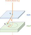 |
Fig. 1. Sketch of a Compton interaction in a Compton telescope. We show the initial photon energy (E0), the recoil electron energy (E1), the scattered photon energy (E2), the polar angle (θ), and the azimuthal angle (ϕ). |
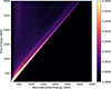 |
Fig. 2. IBIS/Compton RMF with a saturation value for better contrast. |
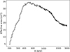 |
Fig. 3. IBIS/Compton ARF. |
where A is the ARF, R is the RMF, B is a boolean rebinning matrix to match the energy channels between the response and spectrum, the dot is the usual matrix multiplication, and the cross is a term-by-term product. This operation is summarized by the operator ℛ. This model count rate is then fit to the energy deposit spectrum determined previously in order to find the true source spectrum.
2.4. Polarimetry
While the scattering angle depends on the energy deposits, the azimuthal angle ϕ depends on the polarization (electric field) direction of the source photons. For a single photon with its electric field in the Ψ0 direction, the Compton cross section depends on the azimuthal angle according to the Klein-Nishina formula,
![Mathematical equation: $$ \begin{aligned} \frac{\mathrm{d}\sigma _C}{\mathrm{d}\Omega } = \frac{r_e^2}{2} \left(\frac{E_2}{E_0}\right)^2 \left[\frac{E_2}{E_0} + \frac{E_0}{E_2} - 2 \sin ^2\theta \cos ^2(\phi -\Psi _0) \right], \end{aligned} $$](/articles/aa/full_html/2026/03/aa58466-25/aa58466-25-eq3.gif) (3)
(3)
where re is the classical electron radius, E0 is the incident photon energy, E2 is the scattered photon energy, and θ is the scattering angle.
For a polarized beam of photons, the expected azimuthal angle distribution deduced from the Klein-Nishina formula, called polarigram, is
 (4)
(4)
where N(ϕ) is the azimuthal angle-dependent count rate in units of counts.s−1.rad−1; this angle rate is independent of the number of angle bins. C is the mean angle rate, a0 the modulation amplitude, and ϕ0 is the preferred azimuthal angle.
This distribution is π-periodic, meaning that we can convert the azimuthal angle of each photon with ϕi → ϕimodπ to focus on the [0, π] interval alone. This has the advantage of removing unwanted 2π-periodic modulations in the signal that might appear due to the geometry of the detector, without changing the polarization signature. Moreover, the number of photons per angle is effectively doubled, resulting in a higher S/N in each angle bin.
In order to measure N(ϕ), the Compton events were sorted according to their azimuthal angle and gathered into np polarization bins by dividing the interval from 0 to π equally. Similarly to what is done for spectra, these distinct event lists were used to build an ISGRI image, which was deconvolved to deduce the source flux for each azimuthal angle bin in a given energy band. The flux was divided by the angle bin size, allowing us to build the polarigram, as shown in black in Fig. 4. The data points above 180° are simply a copy of those below 180°, and they are only shown for clarity.
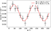 |
Fig. 4. Example of a polarigram fit by Eq. (4). The data used (in black) are from Crab observations in 200–400 keV, summed over the 2003–2016 period (see Section 5.2). |
This method is even more powerful because it enables us to derive independent polarigrams within a given energy range for each detected source in the FOV. Moreover, it can be crucial to choose the correct number of angle bins. In general, a value of np = 6 is the minimum required, and this was used to give lower S/N observation a better detection, that is, a lower minimum detected polarization (MDP). For a high S/N observation, np can be increased for a more accurate polarization angle estimation.
After the measured polarigram was fit with Eq. (4), the polarization angle (PA, or Ψ0) was simply deduced with
 (5)
(5)
and the polarization fraction1 (PF, or Π0) with
 (6)
(6)
where a100 represents the a0 modulation factor when a 100% polarized source is detected. Geant4 simulations of a monochromatic 100% polarized beam made of one million photons allowed us to estimate a100 for many energies between 200 and 3000 keV (see Fig. 5). The statistical fluctuations were largely due to the low efficiency of the Compton scatterings (≈1%), which reduced the number of useful photons for the simulation.
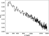 |
Fig. 5. a100 value between 200 and 3000 keV, determined through Geant4 simulations. |
These values were saved in a polarization response file (PRF) and play a similar role as an ARF for the spectra. For a specific energy band [E1,E2], we used a flux-weighted average,
![Mathematical equation: $$ \begin{aligned} a_{100}[E_1,E_2] = \frac{\int _{E_1}^{E_2} a_{100}(E)\,C(E)\, \mathrm{d}E}{\int _{E_1}^{E_2}\,C(E)\, \mathrm{d}E}, \end{aligned} $$](/articles/aa/full_html/2026/03/aa58466-25/aa58466-25-eq7.gif) (7)
(7)
where C(E) is the Compton rate integrated over all ϕ. This removed the need to have prior knowledge of the spectral shape.
An example of a fit polarigram using np = 8 is shown in Fig. 4 using data from the Crab.
2.5. Statistic of polarization
The coded-mask technique means that the individual photon Stokes parameters are not kept during the deconvolution, unlike for other instruments such as IXPE; only the polarization parameters (Π, Ψ) are deduced from the polarigram. The statistic of those parameters is non-Gaussian because the two variables are correlated. Therefore, estimating the confidence intervals (CI) requires some care. The probability of measuring the parameters (Π, Ψ) from the observation of a source with a true polarization (Πs, Ψs) is given by the following probability density function (PDF) (Weisskopf et al. 2009; Quinn 2012):
 (8)
(8)
where we estimated  , following Weisskopf et al. (2009) and Laurent et al. (2011). To test the null-hypothesis, that is, the source being unpolarized (Πs = 0), the PDF was integrated for any angle and above the measured Π = Π0. The p-value is then
 (9)
(9)
When the p-value was above a set threshold, here 1%, the polarization was considered as not detected. An upper limit was found by inverting Equation (9) for a chosen p = plim,
 (10)
(10)
where plim = 1% hereafter.
The uncertainty on the polarization parameters was estimated in the Bayesian framework from a uniform prior by marginalizing the posterior probability distribution (see details in Appendix A). The best values were defined as the mode, and the uncertainties were determined from the highest-density interval (HDI) containing 68%. The main consequences were that the first estimation of Π0 was decreased by a few percent and asymmetrical error bars on Π0. The estimation of Ψ0 remained the same, however, but with larger symmetric error bars. For most measurements in this paper, the detections are significant enough (σ02/Π02 ≪ 1) for the upper and lower errors on Π0 to be approximately equal.
For the further statistical assessment, the delta-negative log-likelihood (defined in Appendix B) can also be computed to determine 2D contours at different probability levels. This is shown for the same 2003–2016 period as before in Fig. 6.
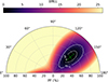 |
Fig. 6. Radar plot of the Crab polarization parameters in the 200–400 keV band. The best parameters are shown with a green cross. The color map shows ΔNLL, with a high-cut value used for better contrast, and the confidence contours are shown with dotted white lines. |
3. The Compton-mode analysis
A workflow chart with the overview of the entire Compton IBIS analysis is given in Appendix C, with all the main interactions of data, software, and simulations. The software is given a list of observation IDs, called SCience Windows (scw), and runs scw by scw from top to bottom for the data analysis part, while the simulations part is ran only once.
3.1. Spurious flux
Unfortunately, some of the double events are not true Compton scattering and are instead spurious events, which correspond to simultaneous detection of two independent source and/or background photons2. As we were unable to distinguish a true Compton photon from a spurious one, we made a global analysis. The main driver of the software is to compute two fluxes: one flux from all double events, and the other flux from the spurious events alone using exactly the same analysis scheme. After subtraction, only the true Compton flux from sources in the FOV remained.
The double events were already gathered in a file, while the list of spurious events was built a posteriori. More precisely, we randomly associated events from the ISGRI and PICsIT single-event files. For ISGRI, this event file is directly created on board, while for PICsIT, this event file is not computed on board and downloaded to Earth because of telemetry limitation. Instead, the PICsIT histogram (a 256-channel spectrum accumulated for each scw and each pixel) was used to generate a PICsIT event file.
As we noted previously, after building this spurious event file, we performed the same analysis for the Compton mode and spurious events in the desired energy band and eventually, for each azimuthal angle bin, to obtain all Compton and spurious source fluxes in the FOV. This computation was similar to the standard INTEGRAL off-line scientific analysis (OSA) software v11.23, with the coded-mask deconvolution being performed on the ISGRI detector image. An additional event selection using the Compton scattering angle θ can be used, but it was not found to change the results significantly and was therefore discarded.
The flux obtained from the spurious events was multiplied by a spurious factor, which remained between 1–3% throughout the mission. This factor gives the probability of two independent events being flagged as Compton events and depends on the ISGRI and PICsIT count rates and on the time coincidence window (Forot et al. 2007). When this spurious flux S was correctly estimated, we subtracted it from the raw Compton flux Cr to determine the true Compton flux Ct,
 (11)
(11)
3.2. Updated energy calibration
The IBIS Compton mode is quite sensitive to the energy calibration, especially below 400 keV, where the ARF and PRF vary substantially. Although the OSA 11 analysis software takes the proper calibration of ISGRI into account, this is not the case for PICsIT. To perform a trustworthy Compton analysis, we first updated its calibration. This was specific to our software, but could still be applied for the PICsIT single events analysis.
As the PICsIT CsI(l) scintillator energy conversion is mostly linear (Malaguti et al. 2003), we used the formula shown below to convert the raw channel number (ci) into energies (Ei) for each photon detected by PICsIT,
![Mathematical equation: $$ \begin{aligned} E_i\,(\mathrm{keV}) = m.\mathrm{gain} .(c_i+U_i{[0,1]}) + \mathrm{offset} , \end{aligned} $$](/articles/aa/full_html/2026/03/aa58466-25/aa58466-25-eq13.gif) (12)
(12)
where the gain and offset are linear coefficients representing the energy conversion from channel number to photon energy, whose physical origins we do not discuss here. m is a factor that accounts for the different binning between the PICsIT single events (in 256 channels) and PICsIT Compton events (in 64 channels). By definition, m = 1 for single and m = 4 for Compton. Ui[0, 1] is a random number drawn from a uniform probability between 0 and 1. It avoids underestimating the energy, which is expected to sit in the middle of the bin (ci + 0.5) on average. It also smooths the spectrum, allowing for a better combination of the spurious and raw Compton events, which have different channel sizes.
For the first three years of the mission, the gain and offset values were deduced from the two radioactive lines of the 22Na IBIS calibration source at 511 keV and 1275 keV (Malaguti et al. 2003). The half-life of the source is 2.5 years, and we therefore installed methods to estimate these values after these lines were no longer detected by PICsIT. These methods were found to be stable during the first three years of the mission, with reliable results, and we therefore assumed that they held for the rest of the mission and ignored possible long-term variations.
3.2.1. PICsIT gain
In Bouchet et al. (2024), we used a fixed gain of 7.1. This can be improved by using the gain-temperature correlation, as it is well known that CsI(Tl) energy response is temperature dependent. In particular, it was shown just after launch that the gain is anticorrelated with the detector temperature (Malaguti et al. 2003). We therefore used this effect to deduce the gain,
![Mathematical equation: $$ \begin{aligned} \mathrm{gain} = a_{T}.T[^{\circ }C] + g_0, \end{aligned} $$](/articles/aa/full_html/2026/03/aa58466-25/aa58466-25-eq14.gif) (13)
(13)
where aT is the slope coefficient, and g0 the gain at T = 0°C. Housekeeping data allowed us to monitor the temperature of each module. By averaging the temperature over all modules during the course of a scw and comparing with the gain measured with the calibration source, we determined these correlation parameters during the first years of the mission. Fig. 7 shows the correlation with an R-value of −0.56, aT = (2.93 ± 0.03).10−2 keV/channel/°C and g0 = 7.287 ± 0.002 keV/channel. The parameters are tightly constrained, as can be seen by the small uncertainties, although there is a high dispersion on T, leading to a weak R-value. This is certainly due to the averaging of the temperature over the entire scw and detector.
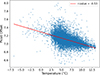 |
Fig. 7. PICsIT detector gain vs. temperature correlation. The data are shown as blue dots, and the model is plotted in red. |
The parameters we found imply a gain variation of ≈0.2%/°C, close to the 0.3%/°C value found in Malaguti et al. (2003). The physical origin of this correlation is most likely related to the light yield dependence of the CsI(Tl) crystal on temperature, which indeed decreases between –25 and 50°C (see Valentine et al. 1993, in particular Fig. 6 and 7).
The uncertainty on the gain (σg) is dominated by the dispersion on T. We made a rough estimate with
 (14)
(14)
with NT the number of data points, and gi and Ti the data points. For average values of the temperature and offset, this results in a dispersion of ≈5.5 keV at 400 keV. For the polarization, this dispersion is smaller than the energy bin sizes used (> 50 keV). On the other hand, this might increase the uncertainty on the calibration parameters, which use smaller energy bins (10 keV). A more precise computation, taking pixel positions and the sub-scw timescale into account, is in preparation.
3.2.2. PICsIT offset
The offset defined in Eq. (12) can be computed from the position of a known line; in our case, the position of the annihilation line produced by the satellite. Cosmic rays constantly interact with the various structures of the satellite, inducing activations and leading to the emission of annihilation photons near 511 keV. This background line can be used in place of the 511 keV line produced by the 22Na source to estimate the PICsIT offset. We used PICsIT events recorded as Compton, grouped into histogram during a single scw, to fit this emission line with a Gaussian. From the channel position of the line and the already known gain, we recovered the offset value.
3.3. Further event selection
There is a discrepancy between the single and double events selection on board. While Compton events are directly transmitted to the on-board data handler unit (OBDH) to be sent on Earth, ISGRI events are first processed, leading to a large portion of them (≈30%) being discarded before transmission to the ground station. In particular, the single ISGRI events that fail certain criteria on the rise time and energy are discarded by the onboard computer to remove false events induced by space protons and to reduce telemetry.
To obtain an accurate estimate of the spurious flux, both types of events need to be treated equally in order to be properly combined. We therefore added a post-selection on the Compton events that mimicked the onboard computer selection using the same criteria and parameters4.
4. Calibration with the Crab
Checking the accuracy of the Compton mode and correcting any discrepancies requires a known calibration source. As stated earlier, there no longer is a radioactive source in IBIS, and we therefore instead relied on the Crab Nebula.
4.1. The Crab, a standard candle for spectroscopy
The Crab is a bright and relatively stable source at high energies that is very frequently observed and used as a telescope calibrator. We used Crab INTEGRAL observations with a maximum off-axis angle of 5° since the PRF was computed for on-axis events. Preliminary tests also showed that 5° was a good compromise for minimum off-axis effects on the polarigrams while maximizing the number of observations for a good S/N (Forot et al. 2008).
INTEGRAL monitored this source regularly during its 22 years of activity (see Fig. 8), amounting to 4663 on-axis scw from June 1, 2003 (MJD 52791) to October 11, 2024 (MJD 60594), equating to 10.9 Ms of exposure. Early observations prior to MJD 52791 had much larger coincidence windows, so we ignored them here for consistency.
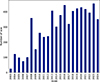 |
Fig. 8. Number of scw with on-axis observation of the Crab, for each year. |
In the soft γ-rays, the INTEGRAL/SPI instrument (Vedrenne et al. 2003) is the most reliable instrument for spectral comparison because its calibration and instrumental response are very stable. The long-term study of the Crab with SPI has shown the light curve and spectra to be stable over time (Jourdain & Roques 2020), which motivated us to use this source as a canonical spectrum.
We relied on the SPI data analysis interface (SPIDAI)5 software to produce a Crab spectrum, which we then fit using the XSpec software (Arnaud 1996). With a power-law model in the 100 keV–1 MeV range, we found a normalization of K = 18.4 ± 4.4 ph.cm−2.s−1.keV−1 at 1 keV and photon index of Γ = 2.24 ± 0.07 (χ2 = 24.55 with 21 d.o.f.).
Although more sophisticated models can be used, namely a broken power law and a Band model, these models are only useful when lower energies are included. In particular, Roques & Jourdain (2019) found a photon index Γ2 = 2.2 − 2.3 for the higher-energy part (Ecut = 100 keV) of their broken power-law model, in agreement with our fit.
4.2. Estimation of the correction parameters
The simple spurious subtraction estimated from the count rates on ISGRI and PICsIT single events has shown some limitations over the mission lifetime. The derived Crab flux strongly deviated over time, above the known intrinsic source variation. To correct the computation of the true Compton flux a posteriori, we introduced new calibration parameters in Eq. 11,
 (15)
(15)
where α are time- and energy-dependent parameters that correct for the raw Compton rate, and β are time-dependent parameters that correct for the spurious rate. In the high-energy range (HE hereafter, defined as E > 350 keV), the β correction is sufficient. The correction for α accounts for the discrepancy in the low-energy range (LE hereafter, defined as E < 350 keV), which is mainly due to the evolution of the ISGRI low-energy threshold with time.
All correction parameters were computed by comparing the Crab spectrum obtained through the IBIS Compton mode and the SPI analysis. This standard procedure, used in high-energy telescopes, was adapted here to correct for the systematic error of the spurious flux estimation becausce this is a critical step of the analysis.
4.2.1. Spurious correction factor
The first step only focused on the HE part of the spectrum. To determine the accurate correction, we compared the IBIS/Compton and SPI (taken as canonical) spectra of the Crab and determined the value of β that minimized the difference. We used the Levenberg-Marquardt (LM) algorithm, which minimizes the χ2 function, but instead of finding spectral parameters, the only parameter left free was β. The SPI flux model was converted into count rates by the Compton-response operator ℛ and compared with the observed Compton spectrum. The χ2 is the sum over the energies E of the fit, chosen between 350 keV and 1.5 MeV,
 (16)
(16)
The method was repeated for different periods, and the LM algorithm determined the best-fit β for each. We chose a duration of two years for each period because this allowed for small enough statistical errors while following the variations with time. The resulting evolution is shown in Fig. 9, where β varies between 0.65 and 0.85, roughly following the cosmic-ray background of the satellite (in red) that is measured from the anticoincidence shield (ACS) of SPI. The uncertainty on β, σβ, was determined using the standard least-squares uncertainty evaluation from the covariance matrix.
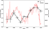 |
Fig. 9. Evolution of the β parameter on the left axis (black), compared with the background count rate on the right axis (SPI/ACS, red). |
4.2.2. Raw Compton correction factor
After we achieved this first correction, we computed the α parameters for the entire energy range. The LE range in particular required a strong correction, which could not be achieved with the β parameters alone. We used Eq. (15) to isolate α, and used the SPI model as a reference by setting Ct = ℛ(Fmod). For a specific period, we had
 (17)
(17)
The uncertainty on α was found by differentiating Eq. 17 with respect to the raw Compton rate and corrected spurious rate (βS), and propagating the errors to α. For the 2013–2015 period, the evolution with energy is shown in Fig. 10. As expected, β alone is sufficient above 350 keV, and therefore, α stays close to 1 with an amplitude variation smaller than ±0.1. In the LE, α is well below 1 and thus compensates for the excess of flux compared to the model. The variation with time of some energy bands is shown in Fig. 11. All parameters seem to decrease until 2010, when it becomes relatively stable. The physical origins of these deviations in energy and time is probably linked to the ISGRI low-threshold evolution, which is still under investigation.
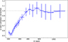 |
Fig. 10. Evolution of the α parameter with energy for the 2013–2015 period. The value α = 1 is shown as a dotted gray line. |
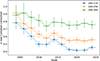 |
Fig. 11. Evolution of the α parameter with time for the first energy bands. |
The α and β parameters were computed once and saved in a table, so the corrected flux was computed during the last step of the Compton-mode analysis. The errors were propagated as follows:
 (18)
(18)
The error on the final flux is dominated by the error terms from σr and σS, while the errors on α and β have an overall negligible effect. We note that the uncertainty on the PICsIT energies (Section 3.2) might also lead to underestimated errors.
4.3. Compton spectrum
To verify the β correction, Compton-mode spectra were built every two years and were fit with a power law between 350 and 1500 keV. In a standard power-law model, the K normalization factor is defined at 1 keV, which is hard to interpret when fitting spectra two orders of magnitude above. Instead, we used the flux in the 350–1000 keV band, F[E1, E2], as the normalization. The power law was rewritten as
![Mathematical equation: $$ \begin{aligned} N(E) = F[E_1,E_2]\,\frac{(\Gamma -2)E^{-\Gamma }}{(E_1^{2-\Gamma }-E_2^{2-\Gamma })}, \end{aligned} $$](/articles/aa/full_html/2026/03/aa58466-25/aa58466-25-eq20.gif) (19)
(19)
where E1 = 350 keV and E2 = 1000 keV. The evolution of the spectral parameters is shown in Fig. 12 compared to SPI values and is listed in Table D.1. Some deviation of Γ is seen at the start of the mission, when the telescope was not yet well calibrated, as well as in the last four years. This behavior is still under study. The flux remained compatible throughout.
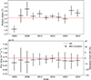 |
Fig. 12. Evolution of the Crab spectral parameters from 300–1500 keV fits. The flux is defined in the 350–1000 keV range. |
A spectrum of the combined dataset is also shown up to 3 MeV in Fig. 13. Using the previous model, we found Γ = 2.28 ± 0.11 and a 350–1000 keV flux of (6.46 ± 0.27) 10−9erg.s−1.cm−2, which agrees well with the SPI model. These results thus confirm that the Compton-mode spectral calibration is sound and can be further used for a polarization analysis.
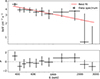 |
Fig. 13. Spectral fit of combined Crab observations in the 2003–2024 period (in red) in the 0.35–3 MeV range. The data-point flux shown in black was estimated using the flux-to-count rate ratio of the model. |
5. Results: Crab polarization
The Crab is the source whose polarization above 1 keV has been measured by the most instruments (see Table 1), followed by Cygnus X-1. The PAs are grouped near the pulsar rotation axis at ΨCP = 124.0 ± 0.1° (Ng & Romani 2004), within roughly ±20°. The PF is measured above 15% and up to 47%, confirming the synchrotron origin of the emission between 1 keV and 1 MeV. Despite these large deviations between the instruments, we used these values for a comparison to our results, keeping in mind that large systematic errors probably exist for some of those experiments.
Summary of 21st century high-energy polarization measurements of the Crab, in chronological order of observation.
5.1. Combined dataset
We used np = 8 for the azimuthal angle binning because it allowed us to have small uncertainties on the polarization parameters while still maintaining a good p value. Combining all data from June 1, 2003 to October 11, 2024 between 200–1000 keV resulted in the polarigram shown in Fig. 14 in black. After fitting and applying the statistical analysis described in Section 5, we found a polarization angle of 128.3 ± 3.8° and a fraction of 50.6 ± 6.6 %.
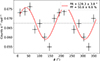 |
Fig. 14. Polarigram of all combined data of the Crab in the 200–1000 keV range. |
This result is shown in black in Fig. 15, compared with other experiments (in colors). The PA is close to the Crab pulsar axis (in gray), while the PF is much higher than the other measurements; it is only compatible with AstroSat. This is likely due to the energy band considered here, which encompasses higher energies than the other experiments, with only AstroSat and SPI having comparable energies. As the Crab polarization has been shown to change with time (Moran et al. 2016), we also studied its evolution.
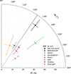 |
Fig. 15. Radar plot of the Crab polarization parameters measured with the IBIS Compton mode in the 200–1000 keV band (black). Other measurements from Table 1 are shown: INTEGRAL/SPI (blue), AstroSat (green), Hitomi (orange), PoGO+ (red), IXPE (purple), XL-Calibur (brown), and PolarLight (pink). The Crab pulsar axis position angle is indicated by a gray line. |
5.2. Crab polarization: Time evolution
The Crab dataset was cut into six periods of roughly equal exposures in order to obtain enough S/N for a detection. We only considered the 200–400 keV band because the detection was not improved when higher-energy bands were included. The results are shown in Table 2, along with the p values.
Crab polarization for different periods measured by the IBIS Compton mode in the 200–400 keV range.
A visual comparison with other missions is shown in Fig. 16. The PA is compatible with most missions, even following the recent variation in angle after MJD 60000 seen by XL-Calibur. The main discrepancy seen is with the SPI measurement before MJD 55000 (in blue), in the early phases of the INTEGRAL mission. The reason might be the calibration of the instruments, which was not settled in this early period. The PF seems larger than most other missions, with only SPI and AstroSat (in green) being compatible. This is probably a difference intrinsic to the source, as the incompatible measurements are all from lower energies (see Table 1). This is corroborated by the fact that the Crab spectrum has a known break around 100 keV (Jourdain & Roques 2020), which might be correlated with a change in polarization behavior. Finally, the variation in time can partially explain the discrepancy seen for the combined dataset.
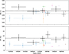 |
Fig. 16. Evolution of Crab polarization measured by IBIS in the 200–400 keV range with the average values shown as dotted black lines and Crab pulsar axis in gray. Other measurements from Table 1 are shown as INTEGRAL/SPI (blue), AstroSat (green), Hitomi (orange), PoGO+ (red), IXPE (purple), XL-Calibur (brown), and PolarLight (pink). |
Crab polarization for the main two periods measured by the IBIS Compton mode.
The previous Crab study by Moran et al. (2016) with IBIS data showed a quite different picture. Their polarization angle in the 300–450 keV range varied from 115 ± 11° to 80 ± 12° between the two time periods of 2003–2007 and 2012–2014. These results were obtained with a different energy calibration and included higher off-axis angle observations. A future study including the phase-resolved Crab polarization, as done by Forot et al. (2008), could shed light on the nature of these differences and determine whether they are of instrumental origin.
Overall, the established relative stability of the Crab spectrum over time (Jourdain & Roques 2020) seems to contradict the large variations in polarization. One explanation would be that only the orientation of the magnetic field at the origin of the synchrotron emission varies, while its strength remains unchanged.
5.3. Evolution with energy
To explore these discrepancies further, we studied the polarization evolution with energy. We separated the dataset into two periods of similar exposures and time span: June 1, 2003 to June 1, 2016 (Period 1), and June 1, 2016 to October 11, 2024 (Period 2), with 4.6 Ms and 6.2 Ms, respectively. Four energy bands were chosen to keep a good S/N (200–250, 250–300, 300–400, and 400–1000 keV), and we only kept other experiments above 100 keV for comparison. The results for both periods are summarized in Table 3 and are shown in Fig. 17.
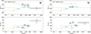 |
Fig. 17. Evolution of the Crab polarization with energy, shown in black. (a) 2003–2016 period. (b) 2016–2024 period. The other missions are INTEGRAL/SPI (blue), AstroSat (green), and Hitomi (orange). |
For Period 1 (left side), polarization is detected in all the energy bands. The PA is nearly constant up to 400 keV and shows a hint of a decrease by ≈20° above 400 keV, but the measurements are still marginally compatible within the errors at 68%. The PF increases with energy, although the errors bars are consistent with each other for the energy bands below 400 keV.
For Period 2, the results are shown in Fig. 17 (right). Polarization is detected only up to 300 keV, with upper limits above 40% for the PF. The PAs between 200–300 keV are compatible with the previous period, while the PF is quite high and decreases between the 200–250 and 250–300 keV band.
The combination of the entire dataset is shown in Fig. 18 and Table 4. The polarization is similar to Period 1, and the only noticeable difference is a lower PF for the 400–1000 keV band. We note that the latter is the highest-energy polarization measurement ever performed for the Crab; it is above 400 keV.
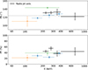 |
Fig. 18. Evolution of the Crab polarization with energy for the entire dataset (2003–2024), shown in black. The other missions are INTEGRAL/SPI (blue), AstroSat (green), and Hitomi (orange). |
Crab polarization measured by the IBIS Compton mode after summing all data from 2003 to 2024.
6. Discussion
The comparison in time and energy of the Crab polarization shows that the IBIS Compton mode does not have strong systematic errors because the data points are mainly compatible with those from similar experiments.
6.1. The polarization fraction
For synchrotron emission, the maximum polarization fraction allowed can be found from the electron power-law distribution (Longair 2011). From the photon index of Γ = 2.24 found in Section 4, the maximum PF is Πmax = 77% for a perfectly ordered magnetic field. All the polarization measurements we found are lower, which further confirms the coherence of our results. The difference in PF is linked with the degree of the order of the underlying magnetic field and can be represented by a multiplicative factor, f = Π0/Πmax (Hughes et al. 1985). For the combined dataset, our measurement results in f = 0.65 ± 0.09 in the 200–1000 keV band, showing only moderate disordering.
Finally, the difference in the polarization fraction between the low (E ≲ 100 keV) and high (E ≳ 100 keV) energies is now firmly established and is shown to persist in time. The change in the spectral behavior around the same energy might indicate a potential explanation. In particular, it was shown that a dependence on energy of the polarization can arise for an electron distribution with a sharp spectral change and a nonuniform pitch-angle distribution (Bjornsson 1985).
6.2. The polarization angle
While the variations in the PF are easily explained by changes in the degree of order, the large discrepancies of the PA (≈20°) are harder to reconcile. If the differences are intrinsic to the source, this implies that there are large changes in the magnetic field configuration, or that different parts of the nebula emit at different times (Moran et al. 2016). This explanation does not hold for the measurements close in time and energy, such as AstroSat and IBIS, since in their cases, the resulting polarization fraction would be lower when integrating over long periods with varying PA.
There might also be larger systematic errors than expected for Astrosat and/or IBIS. The PA of IBIS near MJD 57500 being compatible with POGO+ and SPI, the uncertainties over the polarization angle measured by Astrosat might be underestimated. A pulsar-phase-dependent polarization analysis would help us to decipher this perplexing behavior.
7. Conclusion
We have detailed the complex scheme of the calibration and data analysis of the INTEGRAL/IBIS Compton mode. We showed that the Crab polarization was largely stable between 2003 and 2024, but varied slightly in energy between 200 and 1000 keV. We compared this result with measurements made by others satellites, and we showed that the polarization angle and fraction remained similar.
This also enabled us to produce the first polarization measurement of the Crab strictly above 400 keV. This entirely new polarization constraint might shed light on the emission process and geometry of the source, along with lower-energy measurements. With the new calibration, we are now able to study polarization in the 200 – 300 keV band in detail for the first time, which will expand the number of possible sources to study. The processed product can be analyzed from a publicly available Python library that is described in Appendix E.
As we showed in Section 4, some issues remain in the estimation of the spurious flux in the lower-energy band (below 350 keV). The further improvement of this calibration without introducing ad hoc parameters is still an ongoing work. In particular, this requires an in-depth understanding of the detectors, their electronics, and the onboard data-processing.
It is of the upmost importance in this new era of high-energy polarimetry to obtain reliable results through a rigorous comparison and clear evaluation of systematic effects. The results we presented might in particular be used to assess the sensitivity of future high-energy polarimeters. Table 5 shows a few future missions with polarimetric capabilities that would be able to study the Crab Nebula and pulsar polarization in detail in the same energy range.
Future missions with polarimetric capabilities, with mission status given as of October 2025.
Acknowledgments
We thank the referee for their careful reading and fruitful comments. We acknowledge partial funding from the French Space Agency (CNES). We thank E. Jourdain and J-P.Roques (IRAP) for their help using SPIDAI. We thank A. Sauvageon (CEA) and G. La Rosa (INAF) for their help on the IBIS calibration and satellite onboard selection. Based on observations with INTEGRAL, an ESA project with instruments and science data center funded by ESA member states (especially the PI countries: Denmark, France, Germany, Italy, Switzerland, Spain) and with the participation of Russia and the USA.
References
- Arnaud, K. A. 1996, ASP Conf. Ser., 101, 17 [Google Scholar]
- Awaki, H., Baring, M. G., Bose, R., et al. 2025, MNRAS, 540, L34 [Google Scholar]
- Bjornsson, C. I. 1985, MNRAS, 216, 241 [NASA ADS] [CrossRef] [Google Scholar]
- Bouchet, T., Rodriguez, J., Cangemi, F., et al. 2024, A&A, 688, L5 [NASA ADS] [CrossRef] [EDP Sciences] [Google Scholar]
- Bucciantini, N., Ferrazzoli, R., Bachetti, M., et al. 2023, Nat. Astron., 7, 602 [NASA ADS] [CrossRef] [Google Scholar]
- Cangemi, F., Rodriguez, J., Belloni, T., et al. 2023, A&A, 669, A65 [NASA ADS] [CrossRef] [EDP Sciences] [Google Scholar]
- Chattopadhyay, T. 2021, J. Astrophys. Astron., 42, 106 [Google Scholar]
- Chauvin, M., Florén, H.-G., Friis, M., et al. 2018, MNRAS, 477, L45 [Google Scholar]
- Dean, A. J., Clark, D. J., Stephen, J. B., et al. 2008, Science, 321, 1183 [NASA ADS] [CrossRef] [Google Scholar]
- Feng, H., Li, H., Long, X., et al. 2020, Nat. Astron., 4, 511 [CrossRef] [Google Scholar]
- Forot, M., Laurent, P., Grenier, I. A., Gouiffès, C., & Lebrun, F. 2008, ApJ, 688, L29 [NASA ADS] [CrossRef] [Google Scholar]
- Forot, M., Laurent, P., Lebrun, F., & Limousin, O. 2007, ApJ, 668, 1259 [NASA ADS] [CrossRef] [Google Scholar]
- Franel, N., Tatischeff, V., Murphy, D., et al. 2026, Particles, 9, 13 [Google Scholar]
- Giacconi, R., Gursky, H., Paolini, F. R., & Rossi, B. B. 1962, Phys. Rev. Lett., 9, 439 [NASA ADS] [CrossRef] [Google Scholar]
- Goldwurm, A., David, P., Foschini, L., et al. 2003, A&A, 411, L223 [NASA ADS] [CrossRef] [EDP Sciences] [Google Scholar]
- Goldwurm, A., & Gros, A. 2022, in Handbook of X-ray and Gamma-ray Astrophysics, eds. C. Bambi, & A. Sangangelo, 15 [Google Scholar]
- Götz, D., Covino, S., Fernández-Soto, A., Laurent, P., & Bošnjak, Ž. 2013, MNRAS, 431, 3550 [CrossRef] [Google Scholar]
- Götz, D., Gouiffès, C., Rodriguez, J., et al. 2019, New Astron. Rev., 87, 101537 [CrossRef] [Google Scholar]
- Götz, D., Laurent, P., Antier, S., et al. 2014, MNRAS, 444, 2776 [Google Scholar]
- Götz, D., Laurent, P., Lebrun, F., Daigne, F., & Bosnjak, Z. 2009, ApJ, 695, L208 [CrossRef] [Google Scholar]
- Hitomi Collaboration (Aharonian, F., et al.) 2018, PASJ, 70, 113 [Google Scholar]
- Hughes, P. A., Aller, H. D., & Aller, M. F. 1985, ApJ, 298, 301 [NASA ADS] [CrossRef] [Google Scholar]
- Jourdain, E., & Roques, J. P. 2019, ApJ, 882, 129 [Google Scholar]
- Jourdain, E., & Roques, J. P. 2020, ApJ, 899, 131 [NASA ADS] [CrossRef] [Google Scholar]
- Kumar, R., Carroll, C., Hartikainen, A., & Martin, O. 2019, J. Open Source Software, 4, 1143 [NASA ADS] [CrossRef] [Google Scholar]
- Labanti, C., Di Cocco, G., Ferro, G., et al. 2003, A&A, 411, L149 [NASA ADS] [CrossRef] [EDP Sciences] [Google Scholar]
- Laurent, P., Acero, F., Beckmann, V., et al. 2021, Exp. Astron., 51, 1143 [Google Scholar]
- Laurent, P., Gouiffes, C., Rodriguez, J., & Chambouleyron, V. 2016, in 11th INTEGRAL Conference Gamma-Ray Astrophysics in Multi-Wavelength Perspective, 22 [Google Scholar]
- Laurent, P., Rodriguez, J., Wilms, J., et al. 2011, Science, 332, 438 [Google Scholar]
- Lebrun, F., Leray, J. P., Lavocat, P., et al. 2003, A&A, 411, L141 [NASA ADS] [CrossRef] [EDP Sciences] [Google Scholar]
- Longair, M. S. 2011, High Energy Astrophysics, 3rd edn. (Cambridge University Press) [Google Scholar]
- Malaguti, G., Bazzano, A., Bird, A. J., et al. 2003, A&A, 411, L173 [NASA ADS] [CrossRef] [EDP Sciences] [Google Scholar]
- Moran, P., Kyne, G., Gouiffès, C., et al. 2016, MNRAS, 456, 2974 [Google Scholar]
- Moran, P., Shearer, A., Mignani, R. P., et al. 2013, MNRAS, 433, 2564 [NASA ADS] [CrossRef] [Google Scholar]
- Ng, C. Y., & Romani, R. W. 2004, ApJ, 601, 479 [Google Scholar]
- Quinn, J. L. 2012, A&A, 538, A65 [NASA ADS] [CrossRef] [EDP Sciences] [Google Scholar]
- Rodi, J., Natalucci, L., & Grinta Collaboration 2025, Front. Res. Astrophys, IV, 74 [Google Scholar]
- Rodriguez, J., Grinberg, V., Laurent, P., et al. 2015, ApJ, 807, 17 [NASA ADS] [CrossRef] [Google Scholar]
- Roques, J.-P., & Jourdain, E. 2019, ApJ, 870, 92 [NASA ADS] [CrossRef] [Google Scholar]
- Słowikowska, A., Kanbach, G., Kramer, M., & Stefanescu, A. 2009, MNRAS, 397, 103 [CrossRef] [Google Scholar]
- Tomsick, J., Boggs, S. E., Zoglauer, A., et al. 2019, Am. Astron. Soc. Meeting Abstr., 233, 136.05 [Google Scholar]
- Ubertini, P., Lebrun, F., Di Cocco, G., et al. 2003, A&A, 411, L131 [CrossRef] [EDP Sciences] [Google Scholar]
- Vadawale, S. V., Chattopadhyay, T., Mithun, N. P. S., et al. 2017, Nat. Astron., 2, 50 [NASA ADS] [CrossRef] [Google Scholar]
- Valentine, J. D., Moses, W. W., Derenzo, S. E., Wehe, D. K., & Knoll, G. F. 1993, Nucl. Instrum. Methods Phys. Res. Sect. A, 325, 147 [Google Scholar]
- Vedrenne, G., Roques, J.-P., Schönfelder, V., et al. 2003, A&A, 411, L63 [CrossRef] [EDP Sciences] [Google Scholar]
- Weisskopf, M. C., Elsner, R. F., Kaspi, V. M., et al. 2009, X-Ray Polarimetry and Its Potential Use for Understanding Neutron Stars (Berlin, Heidelberg: Springer), 589 [Google Scholar]
- Zdziarski, A. A., Lubiński, P., & Sikora, M. 2012, MNRAS, 423, 663 [NASA ADS] [CrossRef] [Google Scholar]
- Zhang, H. 2017, Galaxies, 5, 32 [Google Scholar]
Sometimes referred to as the polarization degree (PD), but this might lead to confusion as the angles are usually given in degrees.
Two simultaneous background photons is a case that is already removed through mask deconvolution (see above).
A detailed explanation can be found in the Tübingen University website at https://uni-tuebingen.de/fakultaeten/mathematisch-naturwissenschaftliche-fakultaet/fachbereiche/physik/institute/astronomie-und-astrophysik/astronomie-hea/forschung/abgeschlossene-projekte/integral-ibis/dokumente/
Appendix A: Marginalized posterior estimates
In Bayesian statistics, the posterior probability is the probability of the source having the polarization parameters θ = (Πs,,Ψs) knowing the observation X = (Π0,Ψ0). This probability is computed with the Bayes theorem from the likelihood and the prior distribution. In our case, the prior is uniform for any (Πs, Ψs), and bounded between 0 and 1 for Πs, as a source cannot be polarized above 100%. It is possible, on the other hand, to measure Π0 above 100%, due to statistical fluctuations.
The resulting posterior probability density, ℬ, is almost identical to the PDF, except for Π0 now being treated as a constant,
 (A.1)
(A.1)
where ℬ0 is a normalization factor found by integration. This probability is marginalized on Πs (resp. Ψs), to compute the best value and the HDI at 68% of Ψs (resp. Πs). The best value is defined here as the mode of the marginalized distribution.
A.1. Marginalized posterior on polarization fraction
For the polarization fraction, the distribution is asymmetric. With the strictly positive uniform prior, the integration on Ψs leads to a known solution – the Rice distribution (Weisskopf et al. 2009). The marginalized distribution for Πs is
 (A.2)
(A.2)
where I0 is the zeroth order modified Bessel function of the first kind, and ℳ0 is a normalizing factor found (numerically) by summing the distribution over the [0,1] interval. We sampled this distribution on a fine grid (δΠ = 0.001%) and used the ARVIZ Python library to find the HDI (Kumar et al. 2019), leading to asymmetric errors. The mode is also found at a slightly lower value than the initial Π0, typically by a few percent.
A.2. Marginalized posterior on polarization angle
The marginalized posterior distribution of Ψs, 𝒩, is found by integrating Eq. A.1 between 0 and 1 with respect to Πs. After a few variable changes, and making use of the fact that
 (A.3)
(A.3)
where erf is the error function, we arrive at the analytical formula,
 (A.4)
(A.4)
where y = cos(2(Ψ0 − Ψs)), and 𝒩0 is a normalization factor found by summing the distribution on the [−π/2,π/2] interval. The resulting distribution being symmetric, the errors are simply found by equating a cumulative sum above the mode to 34% (or half of any desired probability). This function being periodic, it can lead to convergence issues if Ψ0 is close to a boundary. To avoid this problem, we set Ψ0 = 0 when computing the error, since the distribution only depends on the difference between the two angles.
Appendix B: Confidence contours
The confidence contours on the 2D plane (Πs, Ψs), are first computed using the negative log-likelihood (NLL),
 (B.1)
(B.1)
where the constant  is the minimum value of the NLL, allowing us to define ΔNLL as
 (B.2)
(B.2)
whose minimum is zero, reached for (Πs = Π0, Ψs = Ψ0). The contour at a desired level pc is found with the χ2 function with 2 degrees of freedom (dof) using Wilk’s theorem approximation,
 (B.3)
(B.3)
Examples for pc = 68 and 99% are shown in Fig. 6.
Appendix C: Workflow chart
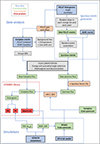 |
Fig. C.1. Workflow chart of the IBIS Compton-mode pipeline. The basic interactions with housekeeping and attitude data are omitted. |
Appendix D: Crab spectral parameters
Evolution of the Crab spectral parameters from the Compton-mode fitting, after β correction.
Appendix E: The COMIBIS Python library
The public python library COMIBIS (contraction of COMpton mode of IBIS) was developed along with notebook examples to facilitate the analysis of raw fluxes. It is available on GitHub6. Users can select INTEGRAL science windows with criteria on dates, satellite revolutions, maximum off-axis angle and energy bands, then create many polarigrams, combine them and show the resulting polarization parameters along with statistical errors. Another module of the library is dedicated to spectral analysis. Similarly to polarization analysis, science windows can be selected and combined to produce spectra between 350 keV and 3 MeV. Those spectra can either be saved as fits, or directly fitted internally with a few basic models.
All Tables
Summary of 21st century high-energy polarization measurements of the Crab, in chronological order of observation.
Crab polarization for different periods measured by the IBIS Compton mode in the 200–400 keV range.
Crab polarization measured by the IBIS Compton mode after summing all data from 2003 to 2024.
Future missions with polarimetric capabilities, with mission status given as of October 2025.
Evolution of the Crab spectral parameters from the Compton-mode fitting, after β correction.
All Figures
|
Fig. 1. Sketch of a Compton interaction in a Compton telescope. We show the initial photon energy (E0), the recoil electron energy (E1), the scattered photon energy (E2), the polar angle (θ), and the azimuthal angle (ϕ). |
| In the text | |
|
Fig. 2. IBIS/Compton RMF with a saturation value for better contrast. |
| In the text | |
|
Fig. 3. IBIS/Compton ARF. |
| In the text | |
|
Fig. 4. Example of a polarigram fit by Eq. (4). The data used (in black) are from Crab observations in 200–400 keV, summed over the 2003–2016 period (see Section 5.2). |
| In the text | |
|
Fig. 5. a100 value between 200 and 3000 keV, determined through Geant4 simulations. |
| In the text | |
|
Fig. 6. Radar plot of the Crab polarization parameters in the 200–400 keV band. The best parameters are shown with a green cross. The color map shows ΔNLL, with a high-cut value used for better contrast, and the confidence contours are shown with dotted white lines. |
| In the text | |
|
Fig. 7. PICsIT detector gain vs. temperature correlation. The data are shown as blue dots, and the model is plotted in red. |
| In the text | |
|
Fig. 8. Number of scw with on-axis observation of the Crab, for each year. |
| In the text | |
|
Fig. 9. Evolution of the β parameter on the left axis (black), compared with the background count rate on the right axis (SPI/ACS, red). |
| In the text | |
|
Fig. 10. Evolution of the α parameter with energy for the 2013–2015 period. The value α = 1 is shown as a dotted gray line. |
| In the text | |
|
Fig. 11. Evolution of the α parameter with time for the first energy bands. |
| In the text | |
|
Fig. 12. Evolution of the Crab spectral parameters from 300–1500 keV fits. The flux is defined in the 350–1000 keV range. |
| In the text | |
|
Fig. 13. Spectral fit of combined Crab observations in the 2003–2024 period (in red) in the 0.35–3 MeV range. The data-point flux shown in black was estimated using the flux-to-count rate ratio of the model. |
| In the text | |
|
Fig. 14. Polarigram of all combined data of the Crab in the 200–1000 keV range. |
| In the text | |
|
Fig. 15. Radar plot of the Crab polarization parameters measured with the IBIS Compton mode in the 200–1000 keV band (black). Other measurements from Table 1 are shown: INTEGRAL/SPI (blue), AstroSat (green), Hitomi (orange), PoGO+ (red), IXPE (purple), XL-Calibur (brown), and PolarLight (pink). The Crab pulsar axis position angle is indicated by a gray line. |
| In the text | |
|
Fig. 16. Evolution of Crab polarization measured by IBIS in the 200–400 keV range with the average values shown as dotted black lines and Crab pulsar axis in gray. Other measurements from Table 1 are shown as INTEGRAL/SPI (blue), AstroSat (green), Hitomi (orange), PoGO+ (red), IXPE (purple), XL-Calibur (brown), and PolarLight (pink). |
| In the text | |
|
Fig. 17. Evolution of the Crab polarization with energy, shown in black. (a) 2003–2016 period. (b) 2016–2024 period. The other missions are INTEGRAL/SPI (blue), AstroSat (green), and Hitomi (orange). |
| In the text | |
|
Fig. 18. Evolution of the Crab polarization with energy for the entire dataset (2003–2024), shown in black. The other missions are INTEGRAL/SPI (blue), AstroSat (green), and Hitomi (orange). |
| In the text | |
|
Fig. C.1. Workflow chart of the IBIS Compton-mode pipeline. The basic interactions with housekeeping and attitude data are omitted. |
| In the text | |
Current usage metrics show cumulative count of Article Views (full-text article views including HTML views, PDF and ePub downloads, according to the available data) and Abstracts Views on Vision4Press platform.
Data correspond to usage on the plateform after 2015. The current usage metrics is available 48-96 hours after online publication and is updated daily on week days.
Initial download of the metrics may take a while.