| Issue |
A&A
Volume 708, April 2026
|
|
|---|---|---|
| Article Number | A91 | |
| Number of page(s) | 10 | |
| Section | The Sun and the Heliosphere | |
| DOI | https://doi.org/10.1051/0004-6361/202557249 | |
| Published online | 26 March 2026 | |
Turbulent acceleration of electrons by large-amplitude magnetohydrodynamic waves in solar flares
Leibniz-Institut für Astrophysik Potsdam, An der Sternwarte 16, D-14482 Potsdam, Germany
★ Corresponding author: This email address is being protected from spambots. You need JavaScript enabled to view it.
Received:
15
September
2025
Accepted:
23
February
2026
Abstract
Context. Solar flares appear as a sudden local enhancement of the emission of electromagnetic waves from the radio to the γ-ray range on the Sun. This radiation is primarily generated by energetic electrons. In addition, these electrons play an important role, since they carry a substantial part of the energy released during a flare. Thus, the generation of highly energetic electrons during flares is one of the basic questions in flare physics. The flare is generally understood as a manifestation of magnetic reconnection in the corona. Several mechanisms of particle acceleration during flares are discussed. Observations and numerical simulations show that a strong magnetohydrodynamic (MHD) turbulence appears in the outflow region of the reconnection site. We consider this turbulence as an ensemble of large-amplitude steepened MHD waves.
Aims. We studied the interaction of electrons with such a wave structure to determine whether the interaction accelerates the electrons.
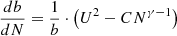
Methods. The properties of the large-amplitude steepened MHD waves are described in terms of simple MHD waves. The interaction of an electron with such a wave structure was treated with a mechanism equivalent to the well-known diffusive shock acceleration.
Results. The multiple interactions of an electron with a large-amplitude steepened MHD waves lead to its continuous acceleration to high energies. The resulting differential electron flux consists of a thermal and a non-thermal component, the latter of which is governed by a power law. The spectral index depends on the density compression within the wave. The stronger the turbulence, the stronger the density compression, and the lower the spectral index. Thus, strong (e.g. GOES M- or X-class) flares are accompanied by strong MHD turbulence in the outflow region of the reconnection site and by a large number of highly relativistic electrons, which are required to account for the solar hard X- and γ-ray radiation.
Conclusions. Strong MHD turbulence in the outflow region of the magnetic reconnection site is able to accelerate electrons to highly relativistic energies.
Key words: Sun: corona / Sun: flares / Sun: particle emission / Sun: X-rays / gamma rays
© The Authors 2026
 Open Access article, published by EDP Sciences, under the terms of the Creative Commons Attribution License (https://creativecommons.org/licenses/by/4.0), which permits unrestricted use, distribution, and reproduction in any medium, provided the original work is properly cited.
This article is published in open access under the Subscribe to Open model. This email address is being protected from spambots. You need JavaScript enabled to view it. to support open access publication.
1. Introduction
On the Sun, a flare occurs as a sudden enhancement of the local emission of electromagnetic waves covering the whole spectrum from the radio to the γ-ray range, with a duration that can reach several hours (see Aschwanden 2005, as a textbook). During flares, a large amount of stored magnetic energy is suddenly released and transferred into the local heating of the coronal plasma, mass motions (e.g. jets), and the generation of energetic particles (usually called solar energetic particle events; see e.g. Lin 1974; Reames et al. 1996; Klein & Trottet 2001; Klein 2021a,b). The flare is considered as a manifestation of magnetic reconnection in the corona. It is currently widely understood in terms of the so-called standard (CSHKP) model (Carmichael 1964; Sturrock 1966; Hirayama 1974; Kopp & Pneuman 1976). According to this model, a filament rises because its photospheric footpoint motions stretch the underlying magnetic field lines and subsequently establish a current sheet. If the current within this sheet exceeds a critical value, plasma waves are excited by different plasma instabilities, leading to an enhancement of the resistivity (see e.g. Treumann & Baumjohann 1997). Then, magnetic reconnection can take place in the region of enhanced resistivity, which is called diffusion region. Due to the strong curvature of the magnetic field lines in the vicinity of the diffusion region, the plasma that slowly inflows to the reconnection site shoots away from the diffusion region and forms the outflow region. During flares, energetic electrons are generated. They travel along the magnetic field lines towards the dense chromosphere, where they emit electromagnetic waves in terms of thick-target bremsstrahlung (Brown 1971) through their interaction with the ambient ions, which are observed as chromospheric hard X-ray sources. Coronal hard X-ray sources are caused by thin-target bremsstrahlung (Lin & Hudson 1976; Hudson et al. 1978). They are especially observed during occulted flares (e.g. Krucker & Lin 2008; Effenberger et al. 2017).
For example, the solar event on September 10, 2017, confirmed the standard (CSHKP) model in an excellent way. It was an X8.2 flare, the second-largest flare in solar cycle 24 (Veronig et al. 2018; Gary et al. 2018; Morosan et al. 2019; Chen et al. 2020; Fleishman et al. 2022; Kontar et al. 2023). This event showed a rising filament with a coronal mass ejection (CME) and an underlying current sheet. Based on microwave imaging with the Expanded Owens Valley Solar Array (EOVSA, Gary et al. 2018), Chen et al. (2020) found that ≈1.6 × 104 cm−3 electrons with energies > 300 keV were produced at the lower end of the current sheet. For this event, Fleishman et al. (2022) derived that a substantial part of all electrons were accelerated to high energies. In contradiction to this result, Kontar et al. (2023) showed for the same event that only a part of about 1% of all electrons were accelerated to energies beyond 20 keV. This result by Kontar et al. (2023) was confirmed for several other events by Volpara et al. (2025). This demonstrates that the generation of energetic electrons is a very hot topic for understanding flares.
Currently, several models for electron acceleration are proposed (see e.g. Chapter 11 in the textbook by Aschwanden 2005, as well as Zharkova et al. 2011 and Mann 2015 as reviews). One model is stochastic acceleration (or wave-particle acceleration) in the turbulent flare region (Parker 1957; Ramaty 1979; Larosa & Moore 1993; Larosa et al. 1996; Miller et al. 1997; Tylka 2001; Petrosian 2012; Bian et al. 2012). Another model is electron acceleration at the so-called termination shock (TS). If the velocity of the plasma in the outflow region becomes super-Alfvénic, a shock wave can be established. This is supported by numerical simulations (Forbes 1986; Forbes & Malherbe 1986; Forbes 1988; Workman et al. 2011; Takasao et al. 2015; Takasao & Shibata 2016; Shen et al. 2018; Kong et al. 2019). Masuda et al. (1994), Shibata et al. (1995), and Tsuneta & Naito (1998) reported on so-called loop-top sources of the hard X-ray (HRX) radiation. The authors proposed that the TS is the source of energetic electrons, which are needed for the HRX emission at the loop-top sources. Mann et al. (2006, 2009) and Warmuth et al. (2009) discussed the generation of energetic electrons at the TS by shock drift acceleration (SDA). Under circumstances in the outflow region, Mann et al. (2024) demonstrated that the plasma is strongly heated at the TS and, thus, provides enough relativistic electrons, as observed in the event on Sep 10, 2017. This model, however, cannot explain the power-law spectrum of the energetic electrons that is produced by the acceleration, as observed. Such a spectrum is necessary to explain γ-ray bursts, which need ultra-relativistic electrons up to the GeV-range (see Chapter 14 in Aschwanden 2005).
The EOVSA observations of the solar event on September 10, 2017 (Gary et al. 2018; Chen et al. 2020), provided strong evidence that the electron acceleration takes place in the outflow region of a flare. This region is filled with a strongly turbulent plasma (Chen et al. 2020). By means of multi-spectral observations, Kontar et al. (2017) and Stores et al. (2021) showed that plasma turbulence may play a key role in the transfer of energy in solar flares. Numerical simulations (Forbes 1986; Forbes & Malherbe 1986; Forbes 1988; Workman et al. 2011; Takasao et al. 2015; Takasao & Shibata 2016; Shen et al. 2018; Kong et al. 2019) also showed that a strong plasma turbulence appears in the outflow region. In a magnetised plasma, strong turbulence is accompanied by large-amplitude fluctuations of the magnetic field and the particle number density.
The quasi-parallel Earth foreshock is the best-studied region of strong plasma turbulence in space (see Russell & Hoppe 1983., as a review) Especially in front of the quasi-parallel Earth bow shock, large-amplitude low-frequency magnetic field fluctuations are observed in form of ultra-low-frequency (ULF) waves and short large-amplitude magnetic field structures (SLAMSs), also called pulsations (Thomsen et al. 1990; Schwartz et al. 1992; Mann et al. 1994). These fluctuations are typically associated with magnetic and density compressions of about Bmax/B0 ≈ 2.4 and Nmax/N0 ≈ 1.4, respectively, and have a spatial full width at half maximum (FWHM) of about 10 ion inertial lengths (Mann et al. 1994). Bmax and Nmax denote the maximum magnetic field strength and particle number density within the SLAM, whereas B0 and N0 are the undisturbed values of these quantities. The properties of SLAMs are theoretically described in terms of so-called simple magnetohydrodynamic (MHD) waves (Mann et al. 1994; Mann 1995).
We adopted the knowledge of these wave structures from Earth bow shock and transferred them to the plasma turbulence in the outflow region of a flare. Thus, we considered the plasma turbulence to consist of a collection of simple MHD waves. Since these waves are accompanied by an enhanced local magnetic field, the multiple interactions of an electron with such a wave accelerates the electron. This mechanism is equivalent to the well-known diffusive shock acceleration.
A brief introduction into the topic of simple MHD waves is presented in Sect. 2. We study the diffusive acceleration of an electron due to its interaction with a simple MHD wave in Sect. 3 The results are used to study the electron acceleration in the outflow region of a flare in Sect. 4. The paper concludes with a short summary (Sect. 5).
2. Introduction into simple MHD waves
We present a brief introduction into simple propagating waves in Riemann’s sense (see Chapter X in Landau & Lifshitz 1966) and their generalisation to simple MHD waves (Shercliff 1960; Mann 1995). In the case of small perturbations, the hydrodynamic equations can be linearised, resulting in a linear wave equation. Its solution is a set of plane-travelling waves that do not change their profile. All varying quantities depend on the spatial coordinate x and the time t only on x ± Wt. Here, W denotes the phase speed of the wave. It is constant in the case of linear waves. In the case of arbitrary amplitudes of the disturbed quantities, there are solutions of plane-travelling waves for which the disturbed quantities are only functions of each other (see Sect. 94 in Chapter X in Landau & Lifshitz 1966). They are usually called simple propagating waves. In contrast to linear waves, these waves change their profile during their evolution (see Fig. 1 for an illustration), leading to wave steepening, and possibly to the establishment of a shock wave due to dissipative processes. The evolution can also lead to wave breaking and to the subsequent annihilation of the wave. The physical quantities (such as the density) change continuously across the simple wave, whereas the shock is basically a discontinuity.
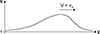 |
Fig. 1. Sketch of a simple wave moving to the right. |
We follow the way presented by Mann (1995). The simple MHD wave propagates along the x-axis and is accompanied by a disturbance of the full particle number density N, the magnetic field B, and the flow velocity v. In the undisturbed region, the full particle number density has the value N0, 0, the magnetic field B0 is placed in the x − z-plane and takes an angle θ towards the x-axis, i.e. B0 = B0(cos θ, 0, sin θ), and the flow speed is given by v0 = ( − v0, 0, 0). The full particle number density N, the magnetic field B, and the flow velocity v are then normalised to N0, 0, B0, and the Alfvén speed 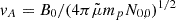 (
( is the mean molecular weight;
  in the solar atmosphere (Priest 1982); mp is the proton mass), respectively. Then, we have
 (1)
(1)
 (2)
(2)
and
 (3)
(3)
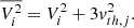
In the case of simple MHD waves, the now normalised disturbances N, b, and ux are related. They can be derived from the ideal MHD equations (see Chapter VIII in Landau & Lifshitz 1975), leading to a non-linear system of differential equations,
 (4)
(4)
 (5)
(5)
with
![Mathematical equation: $$ \begin{aligned} U^{2}&= \frac{1}{2} \left( \frac{b^{2}}{N} + C N^{\gamma - 1} \right) \nonumber \\&+ \sqrt{\frac{1}{4} \left[ \frac{b^{2}}{N}+CN^{\gamma -1} \right]^{2} -C N^{\gamma -2} \cos ^{2} \theta }, \end{aligned} $$](/articles/aa/full_html/2026/04/aa57249-25/aa57249-25-eq9.gif) (6)
(6)
with the initial conditions b(N = 1) = 1 and ux(N = 1) = − u0 (see Eqs. (6b), (7a), and (7b) in Mann (1995), where a detailed derivation of these equations is presented) as well as  and
and  (kB is Boltzmann’s constant, and γ = 5/3 is the ratio of specific heats) as the sound speed of a plasma with a temperature T. In this section, U denotes the wave speed normalised to the Alfvén velocity.
If the simple wave propagates along the magnetic field and C = 0, Eqs. (4), (5), and (6) can be solved analytically,
 (7)
(7)
 (8)
(8)
and
 (9)
(9)
Figure 1 shows a sketch of such a simple wave. It is accompanied by a hump in the density and magnetic field in the case of the fast magnetohydrodynamic mode. The top of the wave propagates with the velocity U + ux, whereas the wings of the wave move with the velocity U(N = 1) = 1. Since the velocities U(N) and ux(N) depend on the full particle number density (see Eqs. (8) and (9)), the peak of the wave moves faster than its wings, leading to a wave steepening, subsequently to the formation of a shock, and finally, to wave breaking and the annihilation of the wave due to dissipative processes. Since the spatial scale becomes smaller in front of the wave, these dissipative processes become important because they act on small spatial scales (see e.g. Treumann & Baumjohann 1997, as a text book).
Now, all velocities are transformed into the rest frame of the wave. Then, we obtain
 (10)
(10)
and
 (11)
(11)
Hence, v1 and v2 represent the flow velocities ahead of and in the inside the wave, respectively.
3. Acceleration of electrons by their interaction with simple MHD waves
The outflow region in a solar flare is characterised by a strong turbulence that is accompanied by strong fluctuations in the density and magnetic field. These fluctuations can be described as an ensemble of so-called simple MHD waves. We treated the interaction of an electron with such a simple MHD wave that accelerates the electron. This mechanism is equivalent to the well-known diffusive shock acceleration. Therefore, we followed the approach presented by Jones (1994) and Gabici (2019) as well as in Chapter 11.5.3 in Aschwanden’s (2005) textbook.
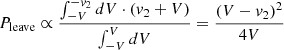
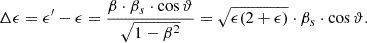
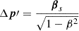
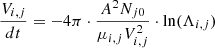
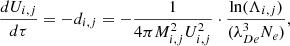
We assumed that the simple MHD waves associated with the strong turbulence in the outflow region of the flare propagate along the ambient magnetic field. Here, the velocities v1 and v2 are the flow velocities ahead of and within the wave (see Eqs. (10) and (11)), respectively. Because v1 > v2, an electron receives an energy gain of
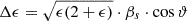 (12)
(12)
at its transition from the region ahead of the wave into its interior (βs = vs/c, vs = v1 − v2, and c is the velocity of light; see Eq. (A.9) and the notations there). Here, ϑ denotes the pitch angle of the electron because the electrons move along the magnetic field in a magnetised plasma. If electrons have the velocity V, then V cos ϑ is the rate at which they can penetrate the wave. Furthermore, the number of electrons with pitch angles in the interval [ϑ, ϑ + dϑ] is proportional to sin ϑ ⋅ dϑ. Then, the probability dppa(ϑ) that an electron with a pitch angle in the interval [ϑ, ϑ + dϑ] can enter the wave is given by
 (13)
(13)
It is normalised to unity, as it should be. When we average over all possible pitch angles, i.e. 0 ≤ ϑ ≤ π/2, the mean energy gain from the transition from the region ahead of the wave into its inside is given by
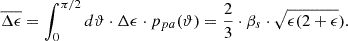 (14)
(14)
In the wave, the electrons experience strong pitch-angle scattering (Treumann & Baumjohann 1997; Jeffrey et al. 2014)1. Thus, the electron can be scattered back into the region ahead of the wave. Then, it receives the same energy gain as during the initial transition from the upstream region into the wave (see p. 27 in Gabici 2019). Hence, its mean energy gain per cycle is found to be
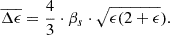 (15)
(15)
Back in the region ahead of the wave, strong pitch-angle scattering, as done by neighbouring simple MHD wave, for example, acts on the electrons so that they can return into the wave.
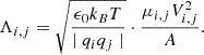
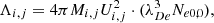
We now introduce P as the probability that the particle persists in the acceleration region. If Ne0 is the initial number density of electrons with an energy ϵ0, then
 (16)
(16)
is the number density of electrons that are available for further acceleration after the kth cycle.
We considered an electron within the simple wave. It propagates with the velocity V along the magnetic field lines. Then, it can enter the region ahead of the wave if V > −v2. Otherwise, it leaves the acceleration region. Hence, the normalised flux of particles that are able to penetrate the upstream region is found to be
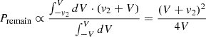 (17)
(17)
(see Eq. (18) in Jones 1994). Furthermore, we obtain
 (18)
(18)
(see Eq. (19) in Jones 1994) for the normalised flux of particles that leave the acceleration region. Hence, the probability P that the particle persists in the acceleration region is given by
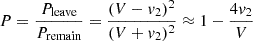 (19)
(19)
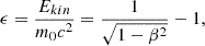
for v2/V ≪ 1 (see Eq. (20) in Jones 1994). This assumption is justified for plasma conditions in the flare region (see the discussion in Sect. 4 and Table 1), since v2 and V are of the order of the Alfvén speed and the thermal electron velocity, respectively, and the thermal electron speed is essentially greater than the Alfvén speed (see Table 1).
Plasma parameters in the outflow region of typical GOES M- and X-class flares.
According to Eqs. (16) and (19), the change in the quantity Ne, k during the (k+1)th cycle can be expressed by
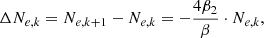 (20)
(20)
with β2 = v2/c and β = V/c. The kth cycle has a duration of Δtk = 2L/cβ. Here, L denotes the distance between the reflection regions located ahead of and within the wave. In these regions, the electrons are scattered back towards the wave and/or into the region ahead of the wave. Then, we obtain a differential equation,
 (21)
(21)
Equation (15) provides the energy gain per cycle, leading to a differential equation
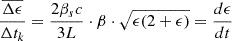 (22)
(22)
with βs = (v1 − v2)/c. Combining Eqs. (21) and (22) with each other,
![Mathematical equation: $$ \begin{aligned} \frac{dN_{e}}{d\epsilon } = - N_{e} \cdot \frac{3\beta _{2}}{\beta } \cdot \frac{(1+\epsilon )}{[\epsilon (2+\epsilon )]} \end{aligned} $$](/articles/aa/full_html/2026/04/aa57249-25/aa57249-25-eq33.gif) (23)
(23)
is obtained, with the solution
![Mathematical equation: $$ \begin{aligned} N_{e}(\epsilon ) = N_{e0} \cdot \left[\frac{\epsilon (2+\epsilon )}{\epsilon _{0}(2+\epsilon _{0})} \right]^{-\alpha }, \end{aligned} $$](/articles/aa/full_html/2026/04/aa57249-25/aa57249-25-eq34.gif) (24)
(24)
with Ne, 0 = N(ϵ = ϵ0) and
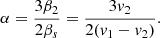 (25)
(25)
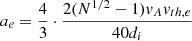
We note that Ne(ϵ) gives the number density of electrons that are accelerated from the initial energy ϵ0 to the final energy ϵ. For high energies, i.e. ϵ ≫ 1, Ne(ϵ) behaves like ∝ϵ−2α. This agrees with the well-known result of diffusive shock acceleration (Jones 1994; Aschwanden 2005).
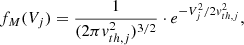
We assumed that the electrons are described by a Maxwellian distribution (see Eq. (A.11)) in the initial state. Then,
 (26)
(26)
me, electron mass) gives the number density of electrons with energies in the interval [ϵ0, ϵ0 + dϵ0] (see Eq. (A.13)). CM is a normalisation constant (see Eq. (A.12)). Ne0, 0 denotes the total electron number density. We obtain from Eq. (24)
![Mathematical equation: $$ \begin{aligned} dN_{e}(\epsilon ) = \left[\frac{\epsilon (2+\epsilon )}{\epsilon _{0}(2+\epsilon _{0})} \right]^{-\alpha } \cdot dN_{e0}. \end{aligned} $$](/articles/aa/full_html/2026/04/aa57249-25/aa57249-25-eq37.gif) (27)
(27)
According to the discussed mechanism, all electrons with an initial energy ϵ0 are accelerated to the energy ϵ. Then, the number density of electrons with energies up to ϵ is found to be
![Mathematical equation: $$ \begin{aligned} N_{e}(\epsilon )&= N_{e0,0}C_{0} \cdot \left[\epsilon (2+\epsilon ) \right]^{-\alpha } \times \nonumber \\&\ \ \int _{\epsilon ^{*}}^{\epsilon } d\epsilon _{0} \left[\epsilon _{0}(2+\epsilon _{0}) \right]^{\alpha +1/2} \cdot (1+\epsilon _{0})e^{-\epsilon _{0}/\epsilon _{th}}, \end{aligned} $$](/articles/aa/full_html/2026/04/aa57249-25/aa57249-25-eq38.gif) (28)
(28)
with C0 = 4π(mec)3CM (see Eq. (A.12)). The thermal core of the initial electron ensemble can be dominated by Coulomb collisions. Only when the acceleration during one cycle of the considered mechanism exceeds the deceleration due to Coulomb collisions (see Appendix B) are the electrons continuously accelerated to higher energies. This can occur when the initial energy of an electron is greater than the energy ϵ*.
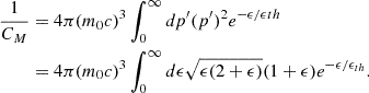
The spectral number density of accelerated electrons is derived to be
![Mathematical equation: $$ \begin{aligned} \frac{dN_{e}}{dE}&= \frac{1}{m_{e}c^{2}} \cdot \frac{dN_{e}}{d\epsilon } \nonumber \\&= \frac{N_{e0,0}C_{0}}{m_{e}c^{2}} \cdot (1+\epsilon ) \cdot [ \sqrt{\epsilon (2+\epsilon )} \cdot e^{-\epsilon /\epsilon _{th}} \nonumber \\&\ \ + 2\alpha \cdot [\epsilon (2+\epsilon )]^{-\alpha -1} \cdot I(\epsilon ) ], \end{aligned} $$](/articles/aa/full_html/2026/04/aa57249-25/aa57249-25-eq39.gif) (29)
(29)
with
![Mathematical equation: $$ \begin{aligned} I(\epsilon ) = \int _{\epsilon ^{*}}^{\epsilon } d\epsilon _{0} \cdot [\epsilon _{0}(2+\epsilon _{0}]^{\alpha +1/2} (1+\epsilon _{0}) e^{-\epsilon _{0}/\epsilon _{th}}. \end{aligned} $$](/articles/aa/full_html/2026/04/aa57249-25/aa57249-25-eq40.gif) (30)
(30)
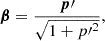
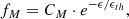
Here, E denotes the kinetic energy of an electron with the velocity V. It is defined by E = mec2[(1 − β2)−1/2 − 1], with β = V/c and the electron rest mass me (see also Eq. (A.3)).
The spectral (or differential) particle flux is usually defined by
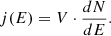 (31)
(31)
Inserting Eq. (29) into Eq. (31), we obtain
![Mathematical equation: $$ \begin{aligned} \frac{j_{e}(E)}{j_{0}} = C_{0} \cdot \left[ \epsilon (2+\epsilon ) \cdot e^{\epsilon /\epsilon _{th}} +2\alpha [\epsilon (2+\epsilon )]^{-(\alpha +1/2)} \cdot I(\epsilon ), \right] \end{aligned} $$](/articles/aa/full_html/2026/04/aa57249-25/aa57249-25-eq42.gif) (32)
(32)
with j0 = Ne0, 0c/mec2. The first term of Eq. (32) is the thermal component of the differential electron flux, whereas the second term describes the component of the accelerated electrons. The spectral flux of accelerated electrons is governed by a power law, as expected for diffusive shock acceleration (Jones 1994; Aschwanden 2005). In the low (i.e. ϵ ≪ 1) and high (i.e. ϵ ≫ 1) energy range, it behaves like ∝ϵ−α − 1/2 and ∝ϵ−2α − 1, respectively.
The basic reason of acceleration in the case of diffusive shock acceleration is that there is a difference in the flow velocities in the up- and downstream region of the shock. Thus, a particle can gain energy by multiple transitions from the up- into the downstream region and back. This is also the case for simple MHD waves, since the flow velocity is lower within the wave than outside. However, in contrast to shocks, where the density jump across the shock is limited to four (see e.g. Priest 1982), there is no density jump in the case of simple MHD waves, but the density is continuously compressed within the wave because a shock wave is a dissipative structure, whereas a simple wave is a purely non-linear structure. Simple MHD waves are described by the ideal MHD equations, which do not contain any dissipative effects (see Sect. 2). Hence, this density compression is basically not limited as in the case of shocks (Mann 1995).
4. Discussion
In the previous section, we presented a model of electron acceleration through interaction of an electron with large-amplitude steepened wave structures. These structures are considered to be the elementary entities of strong MHD turbulence in the outflow region of a flare. The multiple interactions of an electron with such large-amplitude steepened wave structures leads to its continuous acceleration. The differential electron flux resulting from this mechanism is given by Eq. (32). It consists of a thermal and a non-thermal component. The non-thermal component behaves like a power law, as observed for example by Reuven Ramaty High Energy Solar Spectroscopic Imager (RHESSI) (see e.g. Warmuth & Mann 2016; Effenberger et al. 2017).
We calculated the differential electron fluxes for typical plasma parameters in the flare region. Effenberger et al. (2017) studied a sample of 61 occulted flares. Due to their proximity to the solar limb, these events have the advantage that the height of the thermal HXR loop-top source can be determined accurately. In addition, the occultation of lower-lying loops may reduce the contamination by evaporated chromospheric material2, resulting in measured parameters that are closer to the conditions in the outflow region.
We chose the 13 GOES M-class and 2 X-class flares in the sample to derive representative values of the electron number density and the temperature in the outflow region. For the magnetic field, we assumed 400 G in the flare region (see Kuridze et al. (2019) and Gary et al. (2018) for the event on September 10, 2017). This value agrees with the measured radial behaviour of the magnetic field above active regions (e.g. Fedenev et al. 2023), since flares typically occurred at heights in the range 14–25 Mm above the photosphere (Effenberger et al. 2017). The derived plasma parameters are summarised in Table 1. The plasma parameters in the flare region change from one case to the next and also temporally during a flare. Thus, the plasma parameters presented in Table 1 should only be considered as typical ones.
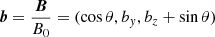
Using the parameters presented in Table 1, we calculated the differential electron fluxes by means of Eq. (32) for typical plasma parameters of M- and X-class flare regions (see Table 1). Warmuth & Mann (2016) derived the spectral indices δ for eight M- and nine X-class flares using RHESSI data. As shown in their Table 3, the spectral indices δ vary between 2.1 and 5.7, with a mean value of 3.7. Inspection of Eq. (32) reveals the relation δ = α + 0.5. Figure 2 shows the thermal component (first term of the right-hand side in Eq. (32); dashed line) in comparison to the non-thermal part (second term of the right-hand side in Eq. (32); full line). It reveals that the non-thermal component becomes dominant beyond 5 keV. Furthermore, Figs. 3 and 4 show the differential electron fluxes for several spectral indices corresponding to typical M- and X-class flare sources, i.e. α = 5.2 (dotted line), α = 1.6 (dashed line), and α = 3.2 (full line), in the energy range 0.001–1.0 MeV and 0.1–100 MeV, respectively. For comparison with observations, we overplotted electron flux densities derived from RHESSI HXR data in Fig. 3. These were obtained from dividing the differential electron flux given by a thick-target fit of a RHESSI spectrum (Warmuth & Mann 2016) by the area of the non-thermal chromospheric footpoints measured from RHESSI images (Warmuth & Mann 2013a). Two cases are shown: the M1.2 flare of April 15, 2002 as an example for a weak M-class flare, and the X8.3 flare of Nov 2, 2003 representing a very strong X-class flare comparable to the event on Sep 10, 2017. In both events, the electron flux density was measured at the peak of the non-thermal HXR emission. Two aspects should be noted here: (1) these are actually lower limits on the flux density since RHESSI probably does not adequately resolve the footpoints (Warmuth & Mann 2013b), and (2) the absolute flux density level in the acceleration region can be different from the level in the footpoints, depending on the magnetic geometry. Nevertheless, Fig. 3 shows that the modelled flux densities are generally consistent with observations.
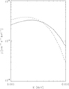 |
Fig. 2. Thermal (dashed line) and non-thermal (full line) component of the differential electron flux for typical GOES M- and X-class flares (see Eq. (32) with α = 3.2) in the energy range 0.001–0.01 MeV. The fluxes are given in cm−2 s−1 keV−1. |
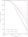 |
Fig. 3. Differential electron fluxes for typical GOES M- and X-class flares in the energy range 0.001–1.0 MeV. We show the modelled fluxes for α = 5.2 (dotted line), α = 1.6 (dashed line), and α = 3.2 (full black line). We overplot the differential electron fluxes for the non-thermal peaks of a small M-class flare (blue line) and a large X-class flare (red line) as derived from RHESSI HXR data. For details, see main text. |
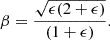
The spectral index α is given by Eq. (25). Since  in the flare plasma (see Table 1), it is justified to describe the simple MHD waves for the case C = 0, as done in Sect. 2. Thus, we obtain for
 (33)
(33)
by means of Eqs. (10) and (11). For α = 5.2, 3.2, and 1.6, we obtain N = 1.37, 1.71, and 3.54, respectively, by means of inverting Eq. (33). In the cases N → 1 and N → ∞, we have α → ∞ and α = 3/4, respectively. There is no turbulence for N = 1, and consequently, no acceleration (i.e. α = ∞). Since a simple MHD wave is accompanied by a local density compression, Eq. (33) reveals that the stronger the turbulence, the stronger the density compression, and, hence, the lower the spectral index (or α). Warmuth & Mann (2016) investigated the relation between the spectral index δ and the peak of the GOES long-channel soft X-ray flux FG (see their Fig. 4) and found that δ decreases with increasing FG. This means that a high energy input is accompanied with a high level of turbulence in the flare region, which is connected with waves of high density and magnetic field compression3, and, hence, with lower values of the spectral index δ (or α) (see Eq. (33)).
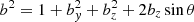
Inspection of Fig. 4 reveals that the spectral index of the electron fluxes changes at about 1 MeV. According to Eq. (32), the non-thermal differential electron flux behaves like ϵ−(α + 1/2) and ϵ−2α − 1 in the range ϵ ≪ 1 and ϵ ≫ 1, respectively.
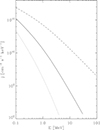 |
Fig. 4. Same as Fig. 2, but showing the modelled differential electron fluxes for α = 5.2 (dotted line), α = 1.6 (dashed line), and α = 3.2 (full black line) in the energy range 0.1–100 MeV. |
In order to compare our theoretical approach with the differential electron fluxes during an individual event, we chose the event on May 15, 2013 (see e.g. Stores et al. 2021), as an example. During the non-thermal peak of this X1.2-class flare (at 01:45 UT), an electron number density Ne = 8.9 × 1010 cm−3 and temperature of T = 22.8 MK were measured by RHESSI in the flare region. In Fig. 5, the differential electron fluxes calculated by means of Eq. (32) with these values for Ne and T are drawn for α = 5.2 (i.e. N = 1.37; dotted line) and 1.6 (i.e. N = 3.54; dashed line). The differential electron flux derived from the hard X-ray spectra obtained by RHESSI is overplotted as a green line in Fig. 5. It reveals that the measured flux agrees with the theoretical flux for α = 5.2. This value of α is related to a typical density compression N = 1.37 due to the turbulence in the flare region.
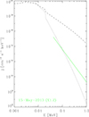 |
Fig. 5. Differential electron flux (green line) for the X1.2-class flare on May 15, 2013, 01:45 UT, as derived from RHESSI data (for details, see main text). The modelled fluxes (see Eq. (32)) are additionally shown for α = 5.2 (dotted line) and α = 1.6 (dashed line). |
According to the presented mechanism, an electron with the initial velocity V experiences an acceleration during one cycle on one hand. On the other hand, it is decelerated due to Coulomb collisions. We discuss these contrary processes below. During one cycle, the electron receives a gain in energy ΔE and travels a distance Δs. Then, the acceleration is found to be
 (34)
(34)
At the beginning of the acceleration process, the electron has a non-relativistic velocity. Hence, Eq. (15) provides for the energy gain
 (35)
(35)
during the first cycle. Inserting Eq. (35) into Eq. (34), we obtain
 (36)
(36)
because of βs = (v1 − v2)/c. By means of Eqs. (10) and (11), we obtain
 (37)
(37)
for V = vth, e. Since a large-amplitude steepened MHD wave has a typical length scale of 20 ion inertial length (di) (Mann et al. 1994), the electron is assumed to travel approximately a distance of 40di during one cycle. In Eq. (37), N denotes the compression of the full particle number density with the wave. As mentioned above, for a typical value of α = 3.2, we obtain N = 1.92. Thus, an electron with the thermal velocity as the initial velocity experiences an acceleration of ai ≈ 1.63 × 1014 cm s−2 during the first cycle4. An electron with a thermal velocity experiences a deceleration of
![Mathematical equation: $$ \begin{aligned} d_{e} = \frac{2\ln [4\pi (\lambda _{De}^{3}N_{e})]}{4\pi (\lambda _{De}N_{e})} \end{aligned} $$](/articles/aa/full_html/2026/04/aa57249-25/aa57249-25-eq49.gif) (38)
(38)
due to Coulomb collision according to Eq. (B.8). Here, de is given as a dimensionless quantity. In order to obtain the deceleration given in terms of cm s−2, Eq. (38) must be multiplied with vth, eωpe according to the normalisation employed in Appendix B. Using the values of the plasma parameters presented in Table 1, we obtain de = 7.5 × 1011 cm s−2. Thus, the acceleration of an electron with thermal energy dominates with respect to its deceleration due to Coulomb collisions. Hence, the choice ϵ* = ϵth = kBT/mec2 in the integral of Eq. (30) is justified, since the thermal core of the electrons can be completely accelerated to high energies.
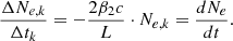
We studied the time tacc that is required to accelerate an electron with an initial energy ϵ0 to the final energy ϵ. Equation (22) describes the temporal evolution of the energy gain. Then, the acceleration time tacc can be derived to be
![Mathematical equation: $$ \begin{aligned} t_{\rm {acc}} = \frac{3L}{4\beta _{s}c} \cdot \ln \left[ \frac{\epsilon (2+\epsilon )}{\epsilon _{0}(2+\epsilon _{0})} \right] \end{aligned} $$](/articles/aa/full_html/2026/04/aa57249-25/aa57249-25-eq50.gif) (39)
(39)
from Eq. (22). As already mentioned, L denotes the mean distance between the reflection points in the upstream region and within the waves. We adopted L as 20di, as in the previous paragraph.
Inspection of Table 2 shows that it takes ≈0.4 ms to accelerate electrons from the thermal energy to 1 GeV. During this time, the electron runs through ≈105 cyclotron periods. These acceleration times are shorter than the temporal resolution of hard X- and γ-ray measurements (see e.g. Chapter 11 in Aschwanden 2005; Miller et al. 1997; Holman et al. 2011; Zharkova et al. 2011). Hence, electrons can be accelerated by the proposed mechanism in the corona within periods shorter than the temporal resolution of current X- and γ-ray instruments. These short timescales might be observed in radio spike bursts (see e.g. Clarkson et al. 2023).
5. Summary
On the Sun, a flare is considered as a manifestation of magnetic reconnection in the solar corona. Observations and numerical simulations both show that a strong MHD turbulence appears in the outflow region of the reconnection site. This turbulence is considered as an ensemble of large-amplitude steepened MHD waves. These wave structures are observed as so-called SLAMS (Mann et al. 1994) in the quasi-parallel Earth foreshock region. They are described in terms of simple MHD waves (Mann 1995). The multiple interaction of an electron with these large-amplitude steepened MHD waves leads to its continual acceleration to high energies (see Sect. 3). This mechanism is equivalent to the diffuse shock acceleration. The differential electron flux resulting from this mechanism (see Eq. (32)) consists of a thermal and a non-thermal component. The latter is governed by a power law, as observed. The power-law index depends on the density compression within the large-amplitude steepened MHD wave (see Eq. (33)). The stronger the turbulence, the stronger the density compression N and the lower the value of α. Thus, strong (e.g. X-GOES-class) flares are accompanied with strong MHD turbulence in the outflow region of the reconnection site. Consequently, they are able to generate highly relativistic electrons, which are required to explain the observed γ-ray radiation during flares, since the value of α is low in these cases. As a result, the relation between the MHD turbulence in the outflow region and the efficiency of electron acceleration is close.
References
- Aschwanden, M. J. 2005, Physics of the Solar Corona. An Introduction with Problems and Solutions, 2nd edn. (Chichester, UK: Praxis Publishing Ltd.) [Google Scholar]
- Bian, N., Emslie, A. G., & Kontar, E. P. 2012, ApJ, 754, 103 [Google Scholar]
- Brown, J. C. 1971, Sol. Phys., 18, 489 [Google Scholar]
- Carmichael, H. 1964, in NASA Special Publication, ed. W. N. Hess, 50, 451 [NASA ADS] [Google Scholar]
- Chen, B., Shen, C., Gary, D. E., et al. 2020, Nat. Astron., 4, 1140 [Google Scholar]
- Clarkson, D. L., Kontar, E. P., Vilmer, N., et al. 2023, ApJ, 946, 33 [NASA ADS] [CrossRef] [Google Scholar]
- Druett, M. K., Ruan, W., & Keppens, R. 2023, Sol. Phys., 298, 134 [NASA ADS] [CrossRef] [Google Scholar]
- Effenberger, F., Rubio da Costa, F., Oka, M., et al. 2017, ApJ, 835, 124 [NASA ADS] [CrossRef] [Google Scholar]
- Estel, C., & Mann, G. 1999, A&A, 345, 276 [NASA ADS] [Google Scholar]
- Fedenev, V. V., Anfinogentov, S. A., & Fleishman, G. D. 2023, ApJ, 943, 160 [NASA ADS] [CrossRef] [Google Scholar]
- Fleishman, G. D., Nita, G. M., Chen, B., Yu, S., & Gary, D. E. 2022, Nature, 606, 674 [NASA ADS] [CrossRef] [Google Scholar]
- Forbes, T. G. 1986, ApJ, 305, 553 [NASA ADS] [CrossRef] [Google Scholar]
- Forbes, T. G. 1988, Sol. Phys., 117, 97 [CrossRef] [Google Scholar]
- Forbes, T. G., & Malherbe, J. M. 1986, ApJ, 302, L67 [NASA ADS] [CrossRef] [Google Scholar]
- Gabici, 2019, The Theory of Diffusive Shock Acceleration, https://apc.u-paris.fr [Google Scholar]
- Gary, D. E., Chen, B., Dennis, B. R., et al. 2018, ApJ, 863, 83 [CrossRef] [Google Scholar]
- Hirayama, T. 1974, Sol. Phys., 34, 323 [Google Scholar]
- Holman, G. D., Aschwanden, M. J., Aurass, H., et al. 2011, Space Sci. Rev., 159, 107 [NASA ADS] [CrossRef] [Google Scholar]
- Hudson, H. S., Canfield, R. C., & Kane, S. R. 1978, Sol. Phys., 60, 137 [Google Scholar]
- Jackson, J. D. 1975, Classical Electrodynamics (New York: Wiley) [Google Scholar]
- Jeffrey, N. L. S., Kontar, E. P., Bian, N. H., & Emslie, A. G. 2014, ApJ, 787, 86 [NASA ADS] [CrossRef] [Google Scholar]
- Jones, F. C. 1994, ApJS, 90, 561 [Google Scholar]
- Klein, K.-L. 2021a, Front. Astron. Space Sci., 7, 105 [NASA ADS] [Google Scholar]
- Klein, K.-L. 2021b, Front. Astron. Space Sci., 7, 93 [NASA ADS] [Google Scholar]
- Klein, K.-L., & Trottet, G. 2001, Space Sci. Rev., 95, 215 [NASA ADS] [CrossRef] [Google Scholar]
- Kong, X., Guo, F., Shen, C., et al. 2019, ApJ, 887, L37 [NASA ADS] [CrossRef] [Google Scholar]
- Kontar, E. P., Perez, J. E., Harra, L. K., et al. 2017, Phys. Rev. Lett., 118, 155101 [NASA ADS] [CrossRef] [Google Scholar]
- Kontar, E. P., Emslie, A. G., Motorina, G. G., & Dennis, B. R. 2023, ApJ, 947, L13 [NASA ADS] [CrossRef] [Google Scholar]
- Kopp, R. A., & Pneuman, G. W. 1976, Sol. Phys., 50, 85 [Google Scholar]
- Krucker, S., & Lin, R. P. 2008, ApJ, 673, 1181 [NASA ADS] [CrossRef] [Google Scholar]
- Kuridze, D., Mathioudakis, M., Morgan, H., et al. 2019, ApJ, 874, 126 [Google Scholar]
- Landau, L. D., & Lifshitz, E. M. 1966, Hydrodynamik (Berlin: Akademie-Verlag) [Google Scholar]
- Landau, L. D., & Lifshitz, E. M. 1975, The Classical Theory of Fields (Oxford: Pergamon Press) [Google Scholar]
- Larosa, T. N., & Moore, R. L. 1993, ApJ, 418, 912 [Google Scholar]
- Larosa, T. N., Moore, R. L., Miller, J. A., & Shore, S. N. 1996, ApJ, 467, 454 [Google Scholar]
- Lin, R. P. 1974, Space Sci. Rev., 16, 189 [NASA ADS] [CrossRef] [Google Scholar]
- Lin, R. P., & Hudson, H. S. 1976, Sol. Phys., 50, 153 [NASA ADS] [CrossRef] [Google Scholar]
- Mann, G. 1995, J. Plasma Phys., 53, 109 [CrossRef] [Google Scholar]
- Mann, G. 2015, J. Plasma Phys., 81, 475810601 [Google Scholar]
- Mann, G., Luehr, H., & Baumjohann, W. 1994, J. Geophys. Res., 99, 13315 [Google Scholar]
- Mann, G., Aurass, H., & Warmuth, A. 2006, A&A, 454, 969 [NASA ADS] [CrossRef] [EDP Sciences] [Google Scholar]
- Mann, G., Warmuth, A., & Aurass, H. 2009, A&A, 494, 669 [NASA ADS] [CrossRef] [EDP Sciences] [Google Scholar]
- Mann, G., Veronig, A. M., & Schuller, F. 2024, A&A, 686, A207 [NASA ADS] [CrossRef] [EDP Sciences] [Google Scholar]
- Masuda, S., Kosugi, T., Hara, H., Tsuneta, S., & Ogawara, Y. 1994, Nature, 371, 495 [CrossRef] [Google Scholar]
- Miller, J. A., Cargill, P. J., Emslie, A. G., et al. 1997, J. Geophys. Res., 102, 14631 [NASA ADS] [CrossRef] [Google Scholar]
- Morosan, D. E., Carley, E. P., Hayes, L. A., et al. 2019, Nat. Astron., 3, 452 [Google Scholar]
- Önel, H., Mann, G., & Sedlmayr, E. 2007, A&A, 463, 1143 [NASA ADS] [CrossRef] [EDP Sciences] [Google Scholar]
- Parker, E. N. 1957, Phys. Rev., 107, 830 [Google Scholar]
- Petrosian, V. 2012, Space Sci. Rev., 173, 535 [NASA ADS] [CrossRef] [Google Scholar]
- Priest, E. R. 1982, in Solar Magneto-hydrodynamics, (Dordrecht, Netherlands: D. Reidel), Geophys. Astrophys. Monogr., 21 [Google Scholar]
- Ramaty, R. 1979, in Particle Acceleration Mechanisms in Astrophysics, eds. J. Arons, C. McKee, & C. Max (AIP), AIP Conf. Ser., 56, 135 [Google Scholar]
- Reames, D. V., Barbier, L. M., & Ng, C. K. 1996, ApJ, 466, 473 [NASA ADS] [CrossRef] [Google Scholar]
- Russell, C. T., & Hoppe, M. M. 1983, Space Sci. Rev., 34, 155 [Google Scholar]
- Schwartz, S. J., Burgess, D., Wilkinson, W. P., et al. 1992, J. Geophys. Res., 97, 4209 [Google Scholar]
- Shen, C., Kong, X., Guo, F., Raymond, J. C., & Chen, B. 2018, ApJ, 869, 116 [NASA ADS] [CrossRef] [Google Scholar]
- Shercliff, J. A. 1960, J. Fluid Mech., 9, 481 [Google Scholar]
- Shibata, K., Masuda, S., Shimojo, M., et al. 1995, ApJ, 451, L83 [Google Scholar]
- Stores, M., Jeffrey, N. L. S., & Kontar, E. P. 2021, ApJ, 923, 40 [Google Scholar]
- Sturrock, P. A. 1966, Nature, 211, 695 [Google Scholar]
- Takasao, S., & Shibata, K. 2016, ApJ, 823, 150 [NASA ADS] [CrossRef] [Google Scholar]
- Takasao, S., Matsumoto, T., Nakamura, N., & Shibata, K. 2015, ApJ, 805, 135 [NASA ADS] [CrossRef] [Google Scholar]
- Thomsen, M. F., Gosling, J. T., Bame, S. J., & Russell, C. T. 1990, J. Geophys. Res., 95, 957 [NASA ADS] [CrossRef] [Google Scholar]
- Treumann, R. A., & Baumjohann, W. 1997, Advanced Space Plasma Physics (London: Imperial College Press) [Google Scholar]
- Tsuneta, S., & Naito, T. 1998, ApJ, 495, L67 [NASA ADS] [CrossRef] [Google Scholar]
- Tylka, A. J. 2001, J. Geophys. Res., 106, 25333 [Google Scholar]
- Veronig, A. M., Podladchikova, T., Dissauer, K., et al. 2018, ApJ, 868, 107 [NASA ADS] [CrossRef] [Google Scholar]
- Volpara, A., Massa, P., Piana, M., Massone, A. M., & Emslie, A. G. 2025, ApJ, 990, 101 [Google Scholar]
- Warmuth, A., & Mann, G. 2013a, A&A, 552, A86 [NASA ADS] [CrossRef] [EDP Sciences] [Google Scholar]
- Warmuth, A., & Mann, G. 2013b, A&A, 552, A87 [NASA ADS] [CrossRef] [EDP Sciences] [Google Scholar]
- Warmuth, A., & Mann, G. 2016, A&A, 588, A115 [NASA ADS] [CrossRef] [EDP Sciences] [Google Scholar]
- Warmuth, A., Mann, G., & Aurass, H. 2009, A&A, 494, 677 [NASA ADS] [CrossRef] [EDP Sciences] [Google Scholar]
- Workman, J. C., Blackman, E. G., & Ren, C. 2011, Phys. Plasmas, 18, 092902 [Google Scholar]
- Zharkova, V. V., Arzner, K., Benz, A. O., et al. 2011, Space Sci. Rev., 159, 357 [Google Scholar]
Large-amplitude steepened MHD wave structures such as SLAMS have a typical spatial extent of about 20 ion inertial lengths (Mann et al. 1994). Hence, there is enough space for embedding whistlers within such a simple MHD wave. It is well-known that whistlers can efficiently cause pitch angle scattering of electrons (Treumann & Baumjohann 1997; Jeffrey et al. 2014).
The energetic electrons generated by the flare can travel along magnetic field lines towards the chromosphere, and hence, they are able to penetrate the chromosphere and heat it, leading to an evaporation of chromospheric material into the corona (e.g. Druett et al. 2023).
According to Eq. (7), a density compression is always connected with a magnetic field compression in the case of a fast simple MHD wave.
Here, the values of vA, vth, e and di given in Table 1 have been used.
Quantities in this system are marked by a prime.
Appendix A: Kinematical relationships in relativistic mechanics
Here, we summarize kinematical relationships, which are employed in Sects. 2 and 3 (see Chapters I and II in Landau & Lifshitz 1975). In relativistic mechanics, the momentum p of a particle with the velocity V and the rest mass m0 is defined by
 (A.1)
(A.1)
with β = V/c (c, velocity of light). The inversion of Eq. (A1) provides
 (A.2)
(A.2)
with p′=p/m0c. The kinetic energy Ekin normalised to the rest energy m0c2 is defined by
 (A.3)
(A.3)
leading to
 (A.4)
(A.4)
Inserting Eq. (A.4) into Eq. (A.2), one gets
 (A.5)
(A.5)
and
 (A.6)
(A.6)
Equation (A.6) is equivalent to the well-known relationship
 (A.7)
(A.7)
If a particle has velocity V in a system of reference, then it has velocity V′
 (A.8)
(A.8)
(with β′=V′/c; β = V/c, and βs = vs/c) in another system 5, which is moving with a velocity vs with respect to the initial one (Landau & Lifshitz 1975). Employing Eq. (A.3), the energy is changed by
 (A.9)
(A.9)
Here, ϑ denotes the angle between V and vs. Then, the momentum of the particle changes by
 (A.10)
during the transition from the initial system of reference to the final one.
In Sect. 2 we assume that the electrons are governed by a Maxwellian distribution:
 (A.11)
with ϵth = kBT/m0c2 (kB, Boltzmann’s constant; T, temperature) in the initial state of the acceleration process. A distribution function is basically defined in the phase space. If the Maxwellian distribution is required to be normalised to unity, CM can be calculated to be
 (A.12)
Here, we took into account that the Maxwellian distribution is isotropic and Eq. (A.6) has been used. In result, the number density of electrons with energies up to ϵ is given by
 (A.13)
with N0, 0 as the undisturbed total particle number density.
Appendix B: Electron deceleration due to Coulomb collisions
In a plasma, an electron experiences a deceleration and a deflection due to its Coulomb interaction with the other electrons and protons. For studying this subject, we follow the approach presented by Jackson (1975), Estel & Mann (1999), and Önel et al. (2007). A particle with velocity Vi, mass mi, and charge qi experiences a deceleration due to Coulomb interaction with a particle with the velocity Vj, mass mj, and charge qj. It is given by
 (B.1)
(B.1)
(see Eq. (8) in Önel et al. 2007) with A = ∣qiqj ∣ /4πϵ0 (ϵ0, dielectric constant), the reduced mass μi, j = mimj/(mi + mj), and
 (B.2)
(B.2)
Here, Nj0 is the undisturbed number density of the particles of the species j.
Vi, j denotes the relative velocity between the particle i with the particle j. If the ensemble of the particles of the species j is described by a Maxwellian distribution function (see Eq. A11):
 (B.3)
(B.3)
with 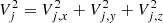 and vth, j = (kBT/mj)1/2 as the thermal speed of the particles of the species j, the mean square of the relative velocity of a particle of the species i with the ensemble of the particle species j is defined by
![Mathematical equation: $$ \begin{aligned} \overline{V_{i}^{2}} = \int dV_{j,x} dV_{j,y} dV_{j,z} \cdot f_{M}(V_{j}) \cdot \left[ (V_{i}-V_{j,x})^{2} + V_{j,y}^{2} + V_{j,z}^{2} \right] .\end{aligned} $$](/articles/aa/full_html/2026/04/aa57249-25/aa57249-25-eq68.gif) (B.4)
(B.4)
Inserting the Maxwellian distribution (B.3) into Eq. (B.4), the integration in Eq. (B.4) provides
 (B.5)
(B.5)
If the particle velocities, the reduced mass, and the time are normalised to the thermal electron velocity vth, e, to the electron mass me, and the inverse of the electron plasma frequency ωpe, i.e. Ui, j = Vi, j/vth, e, Mi, j = μi, j/me, and τ = tωpe, respectively, Eq. (B.1) can be written as
 (B.6)
(B.6)
with
 (B.7)
(B.7)
and with λDe = vth, e/ωpe as the Debye length. Ne0, 0 is the electron number density, which is the same for the protons in an electron-proton plasma. Here, di, j denotes the deceleration of the particle of the species i due to the Coulomb-interaction with the particles of the species j.
The deceleration of an electron with the velocity Ve composes of that due to electron-electron and electron-proton collisions, i.e.
![Mathematical equation: $$ \begin{aligned} d_{e}&= d_{ee} + d_{ep} \nonumber \\&= \frac{1}{4\pi (\lambda _{De}^{3}N_{e0,0})} \left[ \frac{\ln (\Lambda _{ee})}{M_{e,e}^{2}U_{e,e}^{2}} + \frac{\ln (\Lambda _{ep})}{M_{e,p}^{2}U_{e,p}^{2}} \right] \nonumber \\&= \frac{1}{4\pi (\lambda _{De}^{3}N_{e0,0})} \left[ \frac{4\ln (\Lambda _{ee})}{(U_{e}^{2}+3)} + \frac{\ln (\Lambda _{ep})}{U_{e,p}^{2}} \right] ,\end{aligned} $$](/articles/aa/full_html/2026/04/aa57249-25/aa57249-25-eq72.gif) (B.8)
(B.8)
with
![Mathematical equation: $$ \begin{aligned} \ln (\Lambda _{e,e}) = \ln \left[4\pi (\lambda _{De}^{3}N_{e0,0}) \right] + \ln \left[ \frac{(U_{e}^{2}+3)}{2} \right] \end{aligned} $$](/articles/aa/full_html/2026/04/aa57249-25/aa57249-25-eq73.gif) (B.9)
(B.9)
and
![Mathematical equation: $$ \begin{aligned} \ln (\Lambda _{e,p}) = \ln \left[4\pi (\lambda _{De}^{3}N_{e0,0}) \right] + \ln \left[U_{e}^{2} \right] .\end{aligned} $$](/articles/aa/full_html/2026/04/aa57249-25/aa57249-25-eq74.gif) (B.10)
(B.10)
Here, Me, e = 1/2, Me, p = 1,  , and
, and 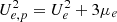 (μe = me/mp; Ue = Ve/vth, e) have been used.
All Tables
All Figures
|
Fig. 1. Sketch of a simple wave moving to the right. |
| In the text | |
|
Fig. 2. Thermal (dashed line) and non-thermal (full line) component of the differential electron flux for typical GOES M- and X-class flares (see Eq. (32) with α = 3.2) in the energy range 0.001–0.01 MeV. The fluxes are given in cm−2 s−1 keV−1. |
| In the text | |
|
Fig. 3. Differential electron fluxes for typical GOES M- and X-class flares in the energy range 0.001–1.0 MeV. We show the modelled fluxes for α = 5.2 (dotted line), α = 1.6 (dashed line), and α = 3.2 (full black line). We overplot the differential electron fluxes for the non-thermal peaks of a small M-class flare (blue line) and a large X-class flare (red line) as derived from RHESSI HXR data. For details, see main text. |
| In the text | |
|
Fig. 4. Same as Fig. 2, but showing the modelled differential electron fluxes for α = 5.2 (dotted line), α = 1.6 (dashed line), and α = 3.2 (full black line) in the energy range 0.1–100 MeV. |
| In the text | |
|
Fig. 5. Differential electron flux (green line) for the X1.2-class flare on May 15, 2013, 01:45 UT, as derived from RHESSI data (for details, see main text). The modelled fluxes (see Eq. (32)) are additionally shown for α = 5.2 (dotted line) and α = 1.6 (dashed line). |
| In the text | |
Current usage metrics show cumulative count of Article Views (full-text article views including HTML views, PDF and ePub downloads, according to the available data) and Abstracts Views on Vision4Press platform.
Data correspond to usage on the plateform after 2015. The current usage metrics is available 48-96 hours after online publication and is updated daily on week days.
Initial download of the metrics may take a while.